Magnonic band structure of a two-dimensional magnetic superlattice

Abstract

The frequencies and linewidths of spin waves in a two-dimensional periodic superlattice of magnetic materials are found, using the Landau-Lifshitz-Gilbert equations. The form of the exchange field from a surface-torque-free boundary between magnetic materials is derived, and magnetic-material combinations are identified which produce gaps in the magnonic spectrum across the entire superlattice Brillouin zone for hexagonal and square-symmetry superlattices.

I Introduction

Advances in the control of spin-wave propagation and dynamicsSerga2010 have led to the demonstration of magnonic bose condensationDemokritov2006 and coupling of electronic spin currents to spin waves in hybrid systemsAndo2011 . Such effects, along with theoretical proposals to electrically-control spin-wave propertiesLiu2011 , and theoretical suggestions of high-temperature operation with small switching energies, may provide the foundation for an information-processing technology based on spin wavesKostylev2005 ; Khitun2010 . Any such technology would benefit from magnetic materials with designed spin-wave dispersion relations, group velocities, and linewidths. A common method of designing such features is the fabrication of a superlattice of different constituent materials, used to design electronic band structures in semiconductor superlattices, and photonic band structures in dielectric superlattices.

Here we focus on the effect of a two-dimensional superlattice of magnetic materials on the magnonic frequencies and linewidths, obtained from a reciprocal-space solution to the Landau-Lifshitz-Gilbert (LLG) equationGilbert2004 . Infinite cylinders of one magnetic material are embedded in a second magnetic material in a periodic arrangement corresponding to a two-dimensional square lattice or hexagonal lattice. Large gaps within the spin-wave spectrum are obtained when the exchange constants and saturation magnetization of the two materials differ greatly; thus the gaps are considerably larger for cylinders of iron embedded within yttrium iron garnet (YIG) than within nickel. For iron embedded in YIG we demonstrate the existence of a gap throughout the superlattice Brillouin zone in the magnon spectrum for both square and hexagonal-symmetry magnonic crystals. In photonic crystals such a feature forms an essential element of photonic band gap materialsYablonovitch1987 ; John1987 , and permits the control of spontaneous emission of emitters embedded within the photonic crystal; here similarly the spontaneous emission of magnons from a source such as a spin-torque nano-oscillator could be suppressed by embedding this spin-wave emitter in a fully-gapped magnonic crystal.

Central to the accurate calculation of dispersion curves associated with a superlattice is the proper treatment of the boundaries between the two magnetic materials. For a magnonic superlattice the exchange field that enters into the LLG equations is discontinuous at the boundary, and that discontinuity strongly influences the spin wave dynamics. Two distinct forms for this exchange field have been described in the literatureVasseur1996 ; Krawczyk2008 ; Tiwari2010 , although to our knowledge it has not been pointed out that these two forms provide dramatically-different solutions to the LLG equation. In Section II we present an explicit derivation of the correct form of the exchange field, followed by spin wave frequencies and linewidths for various magnetic material combinations in Section III. In Section IV we show that solutions to the LLG equations for the incorrect form of the exchange field differ greatly from those for the correct form, and furthermore the incorrect solutions are incompatible with the spatial symmetry of the lattice.

II LLG Formalism for a Quasi-Two-Dimensional Magnonic Crystal

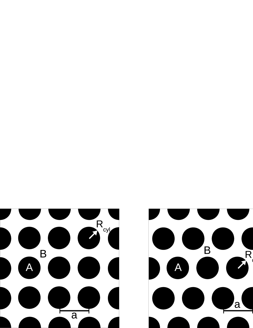
Figure 1: Physical structure of the magnonic crystals studied here. The ferromagnetic material B is the host for infinitely long cylinders of a different ferromagnetic material A arranged in either a square (left) or hexagonal (right) lattice. The lattice constant of the superlattice is $a$ and the cylinder radius is $R_{\rm cyl}$.

We consider a magnonic crystal composed of an array of infinitely long cylinders of ferromagnetic material A embedded in a second ferromagnetic material B in a square or hexagonal lattice; the structures are shown in Fig. 1, and have lattice constant $a$ and cylinder radius $R_{cyl}$. The cylinders are aligned parallel to a static external magnetic field $\mathbf{H_{\mathbf{\mathrm{0}}}}=H_{0}\hat{z}$, and the magnetization of both materials is assumed to be parallel to $\mathbf{H_{\mathbf{\mathrm{0}}}}$. The equation of motion for this system is the Landau-Lifshitz-Gilbert (LLG) equationGilbert2004 :

$$\frac{\partial}{\partial t}\mathbf{M}\left(\mathbf{r},t\right)=\gamma\mu_{0}\mathbf{M}\left(\mathbf{r},t\right)\times\mathbf{H}_{eff}\left(\mathbf{r},t\right)+\frac{\alpha\left(\mathbf{r}\right)}{M_{s}\left(\mathbf{r}\right)}\mathbf{M}\left(\mathbf{r},t\right)\times\frac{\partial}{\partial t}\mathbf{M}\left(\mathbf{r},t\right).$$ (1)

Here $\gamma$ is the gyromagnetic ratio, $M_{s}\left(\mathbf{r}\right)$ is the spontaneous magnetization, $\alpha\left(\mathbf{r}\right)$ is the Gilbert damping parameter, and $\mathbf{r}$ is the three dimensional position vector. The effective magnetic field

$$\mathbf{H}_{eff}\left(\mathbf{r},t\right)=\mathbf{H}_{0}+\mathbf{h}\left(\mathbf{r},t\right)+\mathbf{H}_{ex}\left(\mathbf{r},t\right)$$ (2)

acting on the magnetization $\mathbf{M}\left(\mathbf{r},t\right)$ consists of three terms: the external field $\mathbf{H}_{0}$, the dynamic dipolar field $\mathbf{h}\left(\mathbf{r},t\right)$, and the exchange field $\mathbf{H}_{ex}\left(\mathbf{r},t\right)$.

II.1 Derivation of the Effective Electric Field

We wish to derive the correct form of $H_{eff}\left(\mathbf{r},t\right)$ to use in Eq. (1) for our magnonic crystal. As shown by GilbertGilbert2004 , the exchange field can be obtained by taking the functional derivative of the exchange energy. For a homogeneous material, the exchange energy is Kittel1949

$$U_{ex}\left[\mathbf{M}\left(\mathbf{r}\right)\right]=\frac{A}{M_{s}^{2}}\int\left[\left(\nabla m_{x}\left(\mathbf{r}\right)\right)^{2}+\left(\nabla m_{y}\left(\mathbf{r}\right)\right)^{2}+\left(\nabla m_{z}\left(\mathbf{r}\right)\right)^{2}\right]d\mathbf{r},$$ (3)

where A is the exchange stiffness constant. This yields the following exchange field:

$$\mathbf{H}_{ex}\left(\mathbf{r}\right)=-\frac{1}{\mu_{0}}\frac{\delta U_{ex}\left[\mathbf{M}\left(\mathbf{r}\right)\right]}{\delta\mathbf{M}\left(\mathbf{r}\right)}=\frac{2A}{\mu_{0}M_{s}^{2}}\nabla^{2}\mathbf{M}\left(\mathbf{r}\right).$$ (4)

For the inhomogeneous crystal considered here, the values of the exchange constant and the spontaneous magnetization will differ for the two ferromagnets, so $A$ and $M_{s}$ become spatially dependent quantities:

$$\begin{array}[]{c}A\left(\mathbf{r}\right)=A_{B}+\Theta\left(\mathbf{r}\right)\left(A_{A}-A_{B}\right),\\ M_{s}\left(\mathbf{r}\right)=M_{s_{B}}+\Theta\left(\mathbf{r}\right)\left(M_{s_{A}}-M_{s_{B}}\right),\end{array}$$ (5)

where $\Theta\left(\mathbf{r}\right)=1$ in material A and $\Theta\left(\mathbf{r}\right)=0$ in material B. The exchange energy for this inhomogeneous situation is

$$U_{ex}\left[\mathbf{M}\left(\mathbf{r}\right)\right]=\int A\left(\mathbf{r}\right)\left\{\left[\nabla\left(\frac{m_{x}\left(\mathbf{r}\right)}{M_{s}\left(\mathbf{r}\right)}\right)\right]^{2}+\left[\nabla\left(\frac{m_{y}\left(\mathbf{r}\right)}{M_{s}\left(\mathbf{r}\right)}\right)\right]^{2}+\left[\nabla\left(\frac{m_{z}\left(\mathbf{r}\right)}{M_{s}\left(\mathbf{r}\right)}\right)\right]^{2}\right\}d\mathbf{r},$$ (6)

By approximating the energy with $U_{ex}$ we have neglected non-exchange terms that would give rise to a surface torque (such as terms in the energy associated with surface-induced magnetic anisotropy).

The total magnetization will consist of both a time-dependent term and a time-independent term: $\mathbf{M}\left(\mathbf{r},t\right)=M_{s}\left(\mathbf{r}\right)\hat{z}+\mathbf{m}\left(\mathbf{r},t\right).$ Using the linear magnon approximation we assume that the time-dependent magnetization is small compared to $M_{s}\left(\mathbf{r}\right)$ and therefore we only keep terms up to first order in $\mathbf{m}\left(\mathbf{r},t\right).$ With these assumptions, the inhomogeneous exchange field derived from Eq. (6) is

$$\mathbf{H}_{ex}\left(\mathbf{r},t\right)=\frac{2}{\mu_{0}}\left(\nabla\cdot\frac{A\left(\mathbf{r}\right)}{M_{s}^{2}\left(\mathbf{r}\right)}\nabla\right)\mathbf{M}\left(\mathbf{r},t\right)+\frac{2\mathbf{M}\left(\mathbf{r},t\right)}{\mu_{0}M_{s}\left(\mathbf{r}\right)}\left(\nabla\cdot A\left(\mathbf{r}\right)\nabla\right)\frac{1}{M_{s}\left(\mathbf{r}\right)}\\ -\frac{2\mathbf{m}\left(\mathbf{r},t\right)}{\mu_{0}M_{s}^{2}\left(\mathbf{r}\right)}\cdot\left[\left(\nabla\cdot A\left(\mathbf{r}\right)\nabla\right)\frac{\mathbf{m}\left(\mathbf{r},t\right)}{M_{s}\left(\mathbf{r}\right)}\right]\hat{z}.$$ (7)

The exchange field enters the LLG equation only as a cross product with the magnetization $\mathbf{M}\left(\mathbf{r},t\right)$. The second term is parallel to $\mathbf{M}\left(\mathbf{r},t\right)$ and thus will not contribute to Eq. (1). The third term of Eq. (7), which is proportional to $\mathbf{m}\left(\mathbf{r},t\right)$ and parallel to $M_{s}\left(\mathbf{r}\right)$, will only produce terms of second order in $\mathbf{m}\left(\mathbf{r},t\right)$ in Eq. (1) and can safely be dropped. Therefore, we can approximate

$$\mathbf{H}_{ex}\left(\mathbf{r},t\right)=\frac{2}{\mu_{0}}\left(\nabla\cdot\frac{A\left(\mathbf{r}\right)}{M_{s}^{2}\left(\mathbf{r}\right)}\nabla\right)\mathbf{M}\left(\mathbf{r},t\right),$$ (8)

which produces a LLG equation from Eq. (1) that is correct to first order in $\mathbf{m}\left(\mathbf{r},t\right)$.

We now have the following equation for the effective field:

$$\mathbf{H}_{eff}\left(\mathbf{r},t\right)=H_{0}\hat{z}+\mathbf{h}\left(\mathbf{r},t\right)+\frac{2}{\mu_{0}}\left(\nabla\cdot\frac{A\left(\mathbf{r}\right)}{M_{s}^{2}\left(\mathbf{r}\right)}\nabla\right)\mathbf{M}\left(\mathbf{r},t\right).$$ (9)

This form is a generalization of the boundary condition obtained at the interface between a ferromagnet and vacuumRado1959 , in the absence of any surface torque, and later derived for the boundary condition between dissimilar magnetic materialsHoffmann1970a ; Hoffmann1970b . It is also the form used in Ref. Krawczyk2008, .

II.2 Plane-Wave Solution to LLG Equation for Quasi-Two-Dimensional-Magnonic Crystal

When solving for magnons of a specific frequency $\omega$ we write $\mathbf{m}\left(\mathbf{r},t\right)=\mathbf{m}\left(\mathbf{r}\right)\exp{(-i\omega t)}$ and the dipolar field, $\mathbf{h}\left(\mathbf{r},t\right)=-\nabla\Psi\left(\mathbf{r}\right)\exp{(-i\omega t)}$, with $\Psi\left(\mathbf{r}\right)$ the magnetostatic potential. With the form of the effective field in Eq. (9), the LLG equation (Eq. (1)) can be written

$$i\Omega m_{x}\left(\mathbf{R}\right)+M_{s}\left(\mathbf{R}\right)\nabla\cdot\left(Q\left(\mathbf{x}\right)\nabla m_{y}\left(\mathbf{R}\right)\right)-m_{y}\left(\mathbf{R}\right)\nabla\cdot\left(Q\left(\mathbf{R}\right)\nabla M_{s}\left(\mathbf{R}\right)\right)$$

$$-m_{y}\left(\mathbf{R}\right)-\frac{M_{s}\left(\mathbf{R}\right)}{H_{0}}\frac{\partial\Psi\left(\mathbf{R}\right)}{\partial y}+i\Omega\alpha\left(\mathbf{R}\right)m_{y}\left(\mathbf{R}\right) = 0,$$ (10)

$$i\Omega m_{y}\left(\mathbf{R}\right)-M_{s}\left(\mathbf{R}\right)\nabla\cdot\left(Q\left(\mathbf{R}\right)\nabla m_{x}\left(\mathbf{R}\right)\right)+m_{x}\left(\mathbf{R}\right)\nabla\cdot\left(Q\left(\mathbf{R}\right)\nabla M_{s}\left(\mathbf{R}\right)\right)$$

$$+m_{x}\left(\mathbf{R}\right)+\frac{M_{s}\left(\mathbf{R}\right)}{H_{0}}\frac{\partial\Psi\left(\mathbf{R}\right)}{\partial x}-i\Omega\alpha\left(\mathbf{R}\right)m_{x}\left(\mathbf{R}\right) = 0,$$ (11)

where $\Omega=\omega/(\left|\gamma\right|\mu_{0}H_{0})$ and $Q\left(\mathbf{R}\right)=2A\left(\mathbf{R}\right)/\left(\mu_{0}H_{0}M_{s}^{2}\left(\mathbf{R}\right)\right)$. Additionally, since there is no $z$ dependence in the above equations, the three dimensional position vector $\mathbf{r}$ has been replaced with the two dimensional position vector, $\mathbf{R}=(x,y)$.

This system of equations can be efficiently solved with a plane-wave methodVasseur1996 ; Krawczyk2008 ; Tiwari2010 . We take advantage of the crystal’s periodicity and use Bloch’s theorem to write the magnetization and magnetostatic potential as an expansion of plane waves:

$$\mathbf{m}\left(\mathbf{R}\right)=e^{i\mathbf{k}\cdot\mathbf{R}}\sum_{i}\mathbf{m}_{\mathbf{k}}\left(\mathbf{G}_{i}\right)e^{i\mathbf{G}_{i}\cdot\mathbf{R}},$$ (12)

$$\Psi\left(\mathbf{R}\right)=e^{i\mathbf{k}\cdot\mathbf{R}}\sum_{i}\Psi_{\mathbf{k}}\left(\mathbf{G}_{i}\right)e^{i\mathbf{G}_{i}\cdot\mathbf{R}}.$$ (13)

Here $\mathbf{G}_{i}$ represents a two dimensional reciprocal lattice vector of the crystal and $\mathbf{k}$ is a wave vector in the first Brillouin zone. The magnetostatic potential can be rewritten in terms of the magnetization by using one of Maxwell’s equations:

$$\nabla\cdot\left(\mathbf{h}\left(\mathbf{R}\right)+\mathbf{m}\left(\mathbf{R}\right)\right)=0.$$ (14)

Replacing $\mathbf{h}\left(\mathbf{R}\right)$ with $-\nabla\Psi\left(\mathbf{R}\right)$, substituting in Eqs. (12) and (13), and solving for the potential yields

$$\Psi\left(\mathbf{G}\right)=-i\frac{m_{x,\mathbf{k}}\left(\mathbf{G}\right)\left(\mathbf{G}_{x}+k_{x}\right)+m_{y,\mathbf{k}}\left(\mathbf{G}_{y}+k_{y}\right)}{\left(\mathbf{G}+\mathbf{k}\right)^{2}}.$$ (15)

Next, we need to be able to write the material properties $M_{s}\left(\mathbf{R}\right)$, $Q\left(\mathbf{R}\right)$, and $\alpha\left(\mathbf{R}\right)$ in reciprocal space. Since these have the same periodicity as the crystal lattice, this can be done with a Fourier series expansion:

$$M_{s}\left(\mathbf{R}\right) = \sum_{i}M_{s}\left(\mathbf{G}_{i}\right)e^{i\mathbf{G}_{i}\cdot\mathbf{R}},$$

$$Q\left(\mathbf{R}\right) = \sum_{i}Q\left(\mathbf{G}_{i}\right)e^{i\mathbf{G}_{i}\cdot\mathbf{R},}$$ (16)

$$\alpha\left(\mathbf{R}\right) = \sum_{i}\alpha\left(\mathbf{G}_{i}\right)e^{i\mathbf{G}_{i}\cdot\mathbf{R}}.$$

The Fourier coefficients are obtained by an inverse Fourier transform:

$$M_{s}\left(\mathbf{G}\right) = \frac{1}{S}\int_{S}M_{s}\left(\mathbf{R}\right)e^{-i\mathbf{G}\cdot\mathbf{R}}d^{2}\mathbf{R}.$$ (17)

where S is the area of the two-dimensional unit cell. Performing the integration for $\mathbf{G}=0$ gives the average

$$M_{s}\left(\mathbf{G}=0\right)=M_{s_{A}}f+M_{s_{B}}\left(1-f\right),$$ (18)

where $f$ is the fractional space occupied by a cylinder in the unit cell. For $\mathbf{G}\neq 0$, we have

$$M_{s}\left(\mathbf{G}\neq 0\right)=\left(M_{s_{A}}-M_{s_{B}}\right)2f\frac{J_{1}\left(\left|\mathbf{G}\right|R_{cyl}\right)}{\left|\mathbf{G}\right|R_{cyl}}.$$ (19)

Here $J_{1}$ is a Bessel function of the first kind, and $R_{cyl}$ is the radius of the cylinders. The following infinite system of equations in reciprocal space is obtained by substituting Eqs. (12)-(16) in Eqs. (10) and (11):

$$i\Omega\sum_{j}\left(m_{x,\mathbf{k}}\left(\mathbf{G}_{i}\right)\delta_{ij}+\alpha\left(\mathbf{G}_{i}-\mathbf{G}_{j}\right)m_{y,\mathbf{k}}\left(\mathbf{G}_{j}\right)\right)=\\ \sum_{j}\left\{M_{s}\left(\mathbf{G}_{i}-\mathbf{G}_{j}\right)\frac{\left(G_{x,j}+k_{x}\right)\left(G_{y,j}+k_{y}\right)}{H_{0}\left(\mathbf{G}_{j}+\mathbf{k}\right)^{2}}m_{x,\mathbf{k}}\left(\mathbf{G}_{j}\right)+\left[\delta_{ij}+M_{s}\left(\mathbf{G}_{i}-\mathbf{G}_{j}\right)\frac{\left(G_{y,j}+k_{y}\right)^{2}}{H_{0}\left(\mathbf{G}_{j}+\mathbf{k}\right)^{2}}\right.\right.\\ \left.\left.+\sum_{l}\left(M_{s}\left(\mathbf{G}_{i}-\mathbf{G}_{l}\right)Q\left(\mathbf{G}_{l}-\mathbf{G}_{j}\right)\left(\left(\mathbf{k}+\mathbf{G}_{j}\right)\cdot\left(\mathbf{k}+\mathbf{G}_{l}\right)-\left(\mathbf{G}_{i}-\mathbf{G}_{j}\right)\cdot\left(\mathbf{G}_{i}-\mathbf{G}_{l}\right)\right)\right)\right]m_{y,\mathbf{k}}\left(\mathbf{G}_{j}\right)\right\}$$ (20)

$$i\Omega\sum_{j}\left(m_{y,\mathbf{k}}\left(\mathbf{G}_{i}\right)\delta_{ij}-\alpha\left(\mathbf{G}_{i}-\mathbf{G}_{j}\right)m_{x,\mathbf{k}}\left(\mathbf{G}_{j}\right)\right)=\\ -\sum_{j}\left\{M_{s}\left(\mathbf{G}_{i}-\mathbf{G}_{j}\right)\frac{\left(G_{x,j}+k_{x}\right)\left(G_{y,j}+k_{y}\right)}{H_{0}\left(\mathbf{G}_{j}+\mathbf{k}\right)^{2}}m_{y,\mathbf{k}}\left(\mathbf{G}_{j}\right)+\left[\delta_{ij}+M_{s}\left(\mathbf{G}_{i}-\mathbf{G}_{j}\right)\frac{\left(G_{y,j}+k_{y}\right)^{2}}{H_{0}\left(\mathbf{G}_{j}+\mathbf{k}\right)^{2}}\right.\right.\\ \left.\left.+\sum_{l}\left(M_{s}\left(\mathbf{G}_{i}-\mathbf{G}_{l}\right)Q\left(\mathbf{G}_{l}-\mathbf{G}_{j}\right)\left(\left(\mathbf{k}+\mathbf{G}_{j}\right)\cdot\left(\mathbf{k}+\mathbf{G}_{l}\right)-\left(\mathbf{G}_{i}-\mathbf{G}_{j}\right)\cdot\left(\mathbf{G}_{i}-\mathbf{G}_{l}\right)\right)\right)\right]m_{x,\mathbf{k}}\left(\mathbf{G}_{j}\right)\right\}.$$ (21)

We solve this by limiting the number of reciprocal lattice vectors in the sum and expressing it as a matrix equation:

$$i\Omega\begin{bmatrix}\delta_{ij}&\alpha\left(\mathbf{G}_{i}-\mathbf{G}_{j}\right)\\ \alpha\left(\mathbf{G}_{i}-\mathbf{G}_{j}\right)&\delta_{ij}\end{bmatrix}\begin{bmatrix}m_{x,\mathbf{k}}\left(\mathbf{G}_{1}\right)\\ \vdots\\ m_{x,\mathbf{k}}\left(\mathbf{G}_{N}\right)\\ m_{y,\mathbf{k}}\left(\mathbf{G}_{1}\right)\\ \vdots\\ m_{y,\mathbf{k}}\left(\mathbf{G}_{N}\right)\end{bmatrix}=\begin{bmatrix}B_{ij}^{xx}&B_{ij}^{xy}\\ B_{ij}^{yx}&B_{ij}^{yy}\end{bmatrix}\begin{bmatrix}m_{x,\mathbf{k}}\left(\mathbf{G}_{1}\right)\\ \vdots\\ m_{x,\mathbf{k}}\left(\mathbf{G}_{N}\right)\\ m_{y,\mathbf{k}}\left(\mathbf{G}_{1}\right)\\ \vdots\\ m_{y,\mathbf{k}}\left(\mathbf{G}_{N}\right)\end{bmatrix}$$ (22)

$$B_{ij}^{xx} = -B_{ij}^{yy}=M_{s}\left(\mathbf{G}_{i}-\mathbf{G}_{j}\right)\frac{\left(G_{x,j}+k_{x}\right)\left(G_{y,j}+k_{y}\right)}{H_{0}\left(\mathbf{G}_{j}+\mathbf{k}\right)^{2}}$$ (23)

$$B_{ij}^{xy} = \delta_{ij}+M_{s}\left(\mathbf{G}_{i}-\mathbf{G}_{j}\right)\frac{\left(G_{y,j}+k_{y}\right)^{2}}{H_{0}\left(\mathbf{G}_{j}+\mathbf{k}\right)^{2}}$$ (24)

$$+\sum_{l}M_{s}\left(\mathbf{G}_{i}-\mathbf{G}_{l}\right)Q\left(\mathbf{G}_{l}-\mathbf{G}_{j}\right)\left[\left(\mathbf{k}+\mathbf{G}_{j}\right)\cdot\left(\mathbf{k}+\mathbf{G}_{l}\right)-\left(\mathbf{G}_{i}-\mathbf{G}_{j}\right)\cdot\left(\mathbf{G}_{i}-\mathbf{G}_{l}\right)\right]$$

$$B_{ij}^{yx} = =\delta_{ij}+M_{s}\left(\mathbf{G}_{i}-\mathbf{G}_{j}\right)\frac{\left(G_{x,j}+k_{x}\right)^{2}}{H_{0}\left(\mathbf{G}_{j}+\mathbf{k}\right)^{2}}$$ (25)

$$+\sum_{l}M_{s}\left(\mathbf{G}_{i}-\mathbf{G}_{l}\right)Q\left(\mathbf{G}_{l}-\mathbf{G}_{j}\right)\left[\left(\mathbf{k}+\mathbf{G}_{j}\right)\cdot\left(\mathbf{k}+\mathbf{G}_{l}\right)-\left(\mathbf{G}_{i}-\mathbf{G}_{j}\right)\cdot\left(\mathbf{G}_{i}-\mathbf{G}_{l}\right)\right].$$

The LLG equation is now reduced to finding the eigenvalues and eigenvectors for the above equation.

III Results

From Eq. (22) we calculate the complex eigenvalues $\Omega$ corresponding to the frequencies of magnons in the two-dimensional magnetic superlattices of Fe, Co, Ni, and YIG. The real part of $\Omega_{n}(\mathbf{k})$ is the magnon frequency of branch $n$ for the wave vector $\mathbf{k}$ and the imaginary part is the inverse spin wave lifetime. To focus on the dependence of these properties on magnetic material combinations we consider superlattices with a lattice constant $a=10\mbox{nm}$, an external field $\mu_{0}H_{0}=0.1\mbox{T}$, and a filling fraction $f=0.5$. The material properties, $M_{s}$, $A$, and $\alpha$, are listed in Table 1.

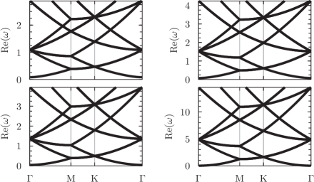
Figure 3: Empty hexagonal lattice band structure obtained from the LLG equation for a homogeneous crystal of Fe (upper left), Co (upper right), Ni (lower left), and YIG (lower right) with lattice constant $a=10\mbox{nm}$. Frequencies are in units of THz.

Figures 2 and 3, show the empty-lattice band structures obtained from the LLG equation for homogeneous crystals of Fe, Co, Ni, and YIG. As the empty-lattice features are governed by the lattice symmetry and the material’s spin wave velocity, these plots depend on material only in setting the frequency scale of the features.

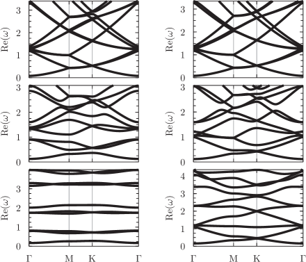
Figure 5: Magnonic band structures for a hexagonal lattice magnonic crystal with lattice spacing $a=10\mbox{nm}$ and filling fraction $f=0.5$. On the left is Fe cylinders embedded in Co (top), Ni (middle), and YIG (bottom). The right is for an Fe host with Co (top), Ni (middle), and YIG (bottom) cylinders. Frequencies are in units of THz.

Figs. 4 and 5 show the results for when Fe is combined with Co, Ni, or YIG. The change in band structure from the homogeneous case is more substantial when there is a greater difference in the spontaneous magnetization between the two materials. For example, the magnetics properties of Fe and Co are fairly similar, and so for a crystal composed of these materials, the band structure differs little from the homogeneous case, with only some small splittings of the spin wave dispersion curves occurring. However, when for a crystal of Fe and YIG, whose magnetizations differ by more than a factor of ten, the magnonic modes are almost completely different from the homogeneous crystal. Furthermore, the opening of band gaps in these structures is more easily attainable when the magnetization is larger in the cylinders than it is in the host. With Fe cylinders embedded in YIG in a square lattice, there are four gaps occurring within the lowest nine spin wave modes, while YIG cylinders in Fe shows only one small gap between the first and second spin wave modes.

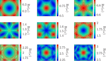
Figure 8: (Color online) The lowest nine spin wave frequencies (in THz) for a hexagonal lattice magnonic crystal composed of Fe cylinders in Ni with a filling fraction of $f=0.5$, and a lattice constant of $a=10\mbox{nm}$. These results were obtained using the exchange field in Eq. (8).

Figs. 6-9 show the detailed dispersion curves and spin wave relaxation rates for a hexagonal superlattice of Fe cylinders in Ni. Plotted are the lowest nine spin wave modes (${\rm Re}\left(\Omega\right)$) in the entire first Brilllouin zone as well as the corresponding inverse spin wave lifetimes (${\rm Im}\left(\Omega\right)$). Quality factors for these modes, corresponding to the ratio of the relaxation rate to the mode frequency, can exceed 100 for such spin waves, especially for the lowest-frequency modes.

IV Comparison with alternate effective field

Some recent calculations of magnonic crystals dispersion curves used a different exchange fieldVasseur1996 ; Tiwari2010 than the one derived in Sec. II. The alternate form,

$$\mathbf{H}_{ex}\left(\mathbf{r},t\right)=\frac{2}{\mu_{0}M_{s}\left(\mathbf{r}\right)}\left(\nabla\cdot\frac{A\left(\mathbf{r}\right)}{M_{s}\left(\mathbf{r}\right)}\nabla\right)\mathbf{M}\left(\mathbf{r},t\right).$$ (26)

differs by the positioning of one factor of $M_{s}\left(\mathbf{r}\right)^{-1}$ outside the gradient operators. A comparison of the band structures obtained for the two different exchange fields is shown in Fig. 10. An examination of the band structure for a homogeneous material composed of Fe or Ni (Fig. 2) indicates that the results for the derived exchanged field (Eq. (8)) produce a band structure that is appreciably different from the homogeneous case, whereas the band structures produced by the alternate exchange field ( Eq. (26)) are very similar to the homogeneous crystal.

In Fig. 11 we show the lowest spin wave mode and corresponding relaxation rate obtained for Fe cylinders in Ni when using Eq. (26) as the exchange field. When looking at these contours, we would expect them to have the same symmetries as the real space lattice. For a square lattice, that would be symmetry under rotations of $90^{\circ}$ and symmetry under reflections about either axis. All symmetries are present for the spin wave modes of Fig. 11, however, the spin wave lifetimes are lacking the reflection symmetries. Comparison with Figs. 6 and 7 shows that the use of Eq. 8 for the exchange field keeps the symmetries of the lattice preserved in the contours. A very slight asymmetry in Figs. 7 and 9 is caused by terminating the infinite summation of the reciprocal lattice vectors in the LLG equation (Eq. (22)), and disappears as the number of reciprocal lattice vectors is increased; the asymmetry in Fig. 11 does not.

Thus the consequences of using the exchange field of Eq. (26) instead of the correct form, Eq. (8), include a dramatic underestimate of the splittings in the magnonic crystal dispersion relations, as well as flawed rotational symmetry of the spin wave relaxation rate.

V Conclusion

Spin wave dispersion curves and relaxation rates have been calculated for hexagonal and square two-dimensional superlattices of magnetic cylinders embedded in another magnetic material. The correct form of the exchange field at the boundary between these two magnetic materials has been found, and the difference from another form used in the literature has been shown to be significant. Full-zone magnonic gaps are obtained for superlattice materials that differ substantially in their saturation magnetization, such as Fe and YIG. Quality factors for spin waves can exceed 100, especially for the lowest-frequency spin mode. These results should assist in the design of magnonic crystals that can focus or redirect spin waves due to their effective band structure.

	$M_{s}\mbox{(A/m)}$	$A\mbox{(pJ/m)}$	$\alpha$
Fe	$1.711\cdot 10^{6}$	$8.3$	$0.0019$
Co	$1.401\cdot 10^{6}$	$10.3$	$0.011$
Ni	$0.485\cdot 10^{6}$	$3.4$	$0.064$
YIG	$0.14\cdot 10^{6}$	$4.15$	$0.0014$

Table 1: Properties of the different materials considered for the magnonic crystalsSkomski2006 ; Oogane2006 ; Slonczewski1974 ; Zhang1996 .

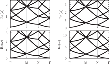
Figure 2: Empty square lattice band structure obtained from the LLG equation for a homogeneous crystal of Fe (upper left), Co (upper right), Ni (lower left), and YIG (lower right) with lattice constant $a=10\mbox{nm}$. Frequencies are in units of THz.

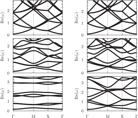
Figure 4: Magnonic band structures for a square lattice magnonic crystal with lattice spacing $a=10\mbox{nm}$ and filling fraction $f=0.5$. On the left is Fe cylinders embedded in Co (top), Ni (middle), and YIG (bottom). The right is for an Fe host with Co (top), Ni (middle), and YIG (bottom) cylinders. Frequencies are in units of THz.

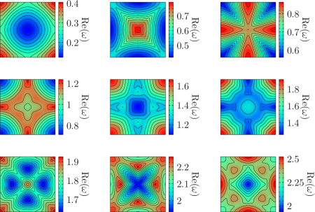
Figure 6: (Color online) The lowest nine spin wave frequencies (in THz) for a square lattice magnonic crystal composed of Fe cylinders in Ni with a filling fraction of $f=0.5$, and a lattice constant of $a=10\mbox{nm}$. These results were obtained using the exchange field in Eq. (8).

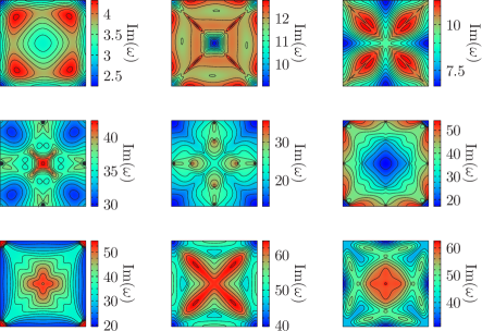
Figure 7: (Color online) The spin wave relaxation rate (in units of GHz) corresponding to the lowest nine spin wave modes from Fig. 6.

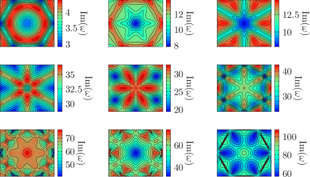
Figure 9: (Color online) The spin wave relaxation rates (in units of GHz) corresponding to the lowest nine spin wave modes from Fig. 8

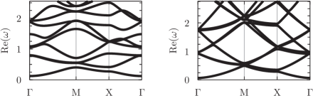
Figure 10: Magnonic band structure of Fe cylinders embedded in Ni calculated from the LLG equation using exchange field in Eq. (8) (left) and Eq. (26) (right). Frequencies are in units of THz.

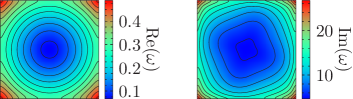
Figure 11: (Color online) The lowest spin wave mode (in THz) and the corresponding relaxation rate (in units of GHz) for a square lattice magnonic crystal composed of Fe cylinders in Ni with a filling fraction of $f=0.5$, and a lattice constant of $a=10\mbox{nm}$. These results were obtained using the exchange field in Eq. (26).

References

• (1) A. A. Serga, A. V. Chumak, and B. Hillebrands, J. Phys. D 43, 264002 (2010)
• (2) S. O. Demokritov, V. E. Demidov, O. Dzyapko, G. A. Melkov, A. A. Serga, B. Hillebrands, and A. N. Slavin, Nature 443, 430 (2006)
• (3) K. Ando, S. Takahashi, J. Ieda, H. Kurebayashi, T. Trypiniotis, C. H. W. Barnes, S. Maekawa, and E. Saitoh, Nature Materials 10, 655 (2011)
• (4) T. Liu and G. Vignale, Phys. Rev. Lett. 106, 247203 (2011)
• (5) M. P. Kostylev, A. A. Serga, T. Schneider, B. Leven, and B. Hillebrands, Appl. Phys. Lett. 87, 153501 (2005)
• (6) A. Khitun, M. Bao, and K. L. Wang, J. Phys. D 43, 264005 (2010)
• (7) T. L. Gilbert, IEEE Trans. Magn. 40, 3443 (2004)
• (8) E. Yablonovitch, Phys. Rev. Lett. 58, 2059 (1987)
• (9) S. John, Phys. Rev. Lett. 58, 2486 (1987)
• (10) J. O. Vasseur, L. Dobrzynski, B. Djafari-Rouhani, and H. Puszkarski, Phys. Rev. B 54, 1043 (Jul 1996)
• (11) M. Krawczyk and H. Puszkarski, Phys. Rev. B 77, 054437 (Feb 2008)
• (12) R. P. Tiwari and D. Stroud, Phys. Rev. B 81, 220403 (Jun 2010)
• (13) C. Kittel, Rev. Mod. Phys. 21, 541 (Oct 1949)
• (14) G. T. Rado and J. R. Weertman, J. Phys. Chem. Solids 11, 315 (1959)
• (15) F. Hoffmann, A. Stankoff, and H. Pascard, J. Appl. Phys. 41, 1022 (1970)
• (16) F. Hoffmann, Phys. Stat. Sol. 41, 807 (1970)
• (17) R. Skomski and D. Sellmyer, Handbook of Advanced Magnetic Materials: Vol 1. Nanostructural Effects (Springer, New York, 2006) p. 20
• (18) M. Oogane, T. Wakitani, S. Yakata, R. Yilgin, Y. Ando, A. Sakuma, and T. Miyazaki, Jpn. J. Appl. Phys. 45, 3889 (May 2006)
• (19) J. C. Slonczewski, A. P. Malozemoff, and E. A. Giess, Appl. Phys. Lett. 24, 396 (Apr 1974)
• (20) Z. Zhang, P. C. Hammel, and P. E. Wigen, Appl. Phys. Lett. 68, 2005 (Jan 1996)