Optimal Lower and Upper Bounds
for Representing Sequences

Abstract

Sequence representations supporting queries $access$, $select$ and $rank$ are at the core of many data structures. There is a considerable gap between the various upper bounds and the few lower bounds known for such representations, and how they relate to the space used. In this article we prove a strong lower bound for $rank$, which holds for rather permissive assumptions on the space used, and give matching upper bounds that require only a compressed representation of the sequence. Within this compressed space, operations $access$ and $select$ can be solved in constant or almost-constant time, which is optimal for large alphabets. Our new upper bounds dominate all of the previous work in the time/space map.

Partially funded by Fondecyt Grant 1-110066, Chile. First author also partially supported by the French ANR-2010-COSI-004 MAPPI Project and the Academy of Finland under grant 250345 (CoECGR).

An early partial version of this work appeared in Proc. ESA’12 [Belazzougui and Navarro (2012)].

Authors’ address: Djamal Belazzougui, Helsinki Institute for Information Technology HIIT, Department of Computer Science, University of Helsinki, Finland, djamal.belazzougui@gmail.com. Gonzalo Navarro, Department of Computer Science, University of Chile, Chile, gnavarro@dcc.uchile.cl

1 Introduction

A large number of data structures build on sequence representations. In particular, supporting the following three queries on a sequence $S[1,n]$ over alphabet $[1,\sigma]$ has proved extremely useful:

• $access(S,i)$ gives $S[i]$;

• $select_{a}(S,j)$ gives the position of the $j$th occurrence of $a\in[1,\sigma]$ in $S$; and

• $rank_{a}(S,i)$ gives the number of occurrences of $a\in[1,\sigma]$ in $S[1,i]$.

The most basic case is that of bitmaps, when $\sigma=2$. Obvious applications are set representations supporting membership and predecessor search, although many other uses, such as representing tree topologies, multisets, and partial sums [Jacobson (1989), Raman et al. (2007)] have been reported. The focus of this article is on general alphabets, where further applications have been described. For example, the FM-index [Ferragina and Manzini (2005)], a compressed indexed representation for text collections that supports pattern searches, is most successfully implemented over a sequence representation supporting $access$ and $rank$ [Ferragina et al. (2007)], and more recently $select$ [Belazzougui and Navarro (2011)]. GGV03 had used earlier similar techniques for text indexing. GMR06 used these operations for representing labeled trees and permutations. Further applications of these operations to multi-labeled trees and binary relations were uncovered by BHMR11. FLMM09, GHSV06, and ACMNNSV10 devised new applications to XML indexing. Other applications were described as well to representing permutations and inverted indexes [Barbay and Navarro (2009), Barbay et al. (2012)] and graphs [Claude and Navarro (2010), Hernández and Navarro (2012)]. VM07 and GNP10 applied them to document retrieval on general texts. Finally, applications to various types of inverted indexes on natural language text collections have been explored [Brisaboa et al. (2012), Arroyuelo et al. (2010b), Arroyuelo et al. (2012)].

When representing sequences supporting the three operations, it seems reasonable to aim for $O(n\lg\sigma)$ bits of space. However, in many applications the size of the data is huge and space usage is crucial: only sublinear space on top of the raw data can be accepted. This is our focus.

Various time- and space-efficient sequence representations supporting the three operations have been proposed, and also various lower bounds have been proved. All the representations proposed assume the RAM model with word size $w=\Omega(\lg n)$. In the case of bitmaps, Mun96 and Cla96 achieved constant-time $rank$ and $select$ using $o(n)$ extra bits on top of a plain representation of $S$. Gol07 proved a lower bound of $\Omega(n\lg\lg n/\lg n)$ extra bits for supporting either operation in constant time if $S$ is to be represented in plain form, and gave matching upper bounds. This assumption is particularly inconvenient in the frequent case where the bitmap is sparse, that is, it has only $m\ll n$ 1s, and hence can be compressed. When $S$ can be represented arbitrarily, Pat08 achieved $\lg{n\choose m}+O(n/\lg^{c}n)$ bits of space, where $c$ is any constant. This space was shown later to be optimal [Pătraşcu and Viola (2010)]. However, the space can be reduced further, up to $\lg{n\choose m}+O(m)$ bits, if superconstant time for the operations is permitted [Gupta et al. (2007), Okanohara and Sadakane (2007)], or if the operations are weakened: When $rank_{1}(S,i)$ can only be applied if $S[i]=1$ and only $select_{1}(S,j)$ is supported, RRR07 achieved constant time and $\lg{n\choose m}+o(m)+O(\lg\lg n)$ bits of space. When only $rank_{1}(S,i)$ is supported for the positions $i$ such that $S[i]=1$, and in addition we cannot even determine $S[i]$, the structure is called a monotone minimum perfect hash function (mmphf) and can be implemented in $O(m\lg\lg\frac{n}{m})$ bits and answering in constant time [Belazzougui et al. (2009)].

For general sequences, a useful measure of compressibility is the zeroth-order entropy of $S$, $H_{0}(S)=\sum_{a\in[1,\sigma]}\frac{n_{a}}{n}\lg\frac{n}{n_{a}}$, where $n_{a}$ is the number of occurrences of $a$ in $S$. This can be extended to the $k$-th order entropy, $H_{k}(S)=\frac{1}{n}\sum_{A\in[1,\sigma]^{k}}|T_{A}|H_{0}(T_{A})$, where $T_{A}$ is the string of symbols following $k$-tuple $A$ in $S$. It holds $0\leq H_{k}(S)\leq H_{k-1}(S)\leq H_{0}(S)\leq\lg\sigma$ for any $k$, but the entropy measure is only meaningful for $k<\lg_{\sigma}n$. See Man01 and Gag06 for a deeper discussion.

We say that a representation of $S$ is succinct if it takes $n\lg\sigma+o(n\lg\sigma)$ bits, zeroth-order compressed if it takes $nH_{0}(S)+o(n\lg\sigma)$ bits, and high-order compressed if it takes $nH_{k}(S)+o(n\lg\sigma)$ bits. We may also compress the redundancy, $o(n\lg\sigma)$, to use for example $nH_{0}(S)+o(nH_{0}(S))$ bits.

Upper and lower bounds for sequence representations supporting the three operations are far less understood over arbitrary alphabets. GGV03 introduced the wavelet tree, a zeroth-order compressed representation using $nH_{0}(S)+o(n\lg\sigma)$ bits that solves the three queries in time $O(\lg\sigma)$. The time was reduced to $O\left(1+\frac{\lg\sigma}{\lg\lg n}\right)$ with multiary wavelet trees [Ferragina et al. (2007)], and later the space was reduced to $nH_{0}(S)+o(n)$ bits [Golynski et al. (2008)]. Note that the query times are constant for $\lg\sigma=O(\lg\lg n)$, that is, $\sigma=O(\mathrm{polylog}~{}n)$. GMR06 proposed a succinct representation that is more interesting for large alphabets. It solves $access$ and $select$ in $O(1)$ and $O(\lg\lg\sigma)$ time, or vice versa, and $rank$ in $O(\lg\lg\sigma)$ time or slightly more. This representation was made slightly faster (i.e., $rank$ time is always $O(\lg\lg\sigma)$) and compressed to $nH_{0}(S)+o(nH_{0}(S))+o(n)$ by BCGNN12. Alternatively, BHMR11 achieved high-order compression, $nH_{k}(S)+o(n\lg\sigma)$ bits for any $k=o(\lg_{\sigma}n)$, and slightly higher times, which were again reduced by GOR10.

There are several curious aspects in the map of the current solutions for general sequences. On the one hand, in various solutions for large alphabets [Golynski et al. (2006), Barbay et al. (2012), Grossi et al. (2010)] the times for $access$ and $select$ seem to be complementary (i.e., one is constant and the other is not), whereas that for $rank$ is always superconstant. On the other hand, there is no smooth transition between the complexity of the wavelet-tree based solutions, $O\left(1+\frac{\lg\sigma}{\lg\lg n}\right)$, and those for larger alphabets, $O(\lg\lg\sigma)$.

The complementary nature of $access$ and $select$ is not a surprise. Gol09 proved lower bounds that relate the time performance that can be achieved for these operations with the redundancy of any encoding of $S$ on top of its information content. The lower bound acts on the product of both times, that is, if $t$ and $t^{\prime}$ are the time complexities for $access$ and $select$, and $\rho$ is the bit-redundancy per symbol, then $\rho\cdot t\cdot t^{\prime}=\Omega((\lg\sigma)^{2}/w)$ holds for a wide range of values of $\sigma$. Many upper bounds for large alphabets [Golynski et al. (2006), Barbay et al. (2012), Grossi et al. (2010)] match this lower bound when $\lg\sigma=\Theta(w)$.

Despite operation $rank$ seems to be harder than the others (at least no constant-time solution exists except for polylog-sized alphabets), no general lower bounds on this operation have been proved. Only a result [Grossi et al. (2010)] for the case in which $S$ must be encoded in plain form states that if one solves $rank$ within $a=O\left(1+\frac{\lg\sigma}{\lg\lg\sigma}\right)$ accesses to the sequence, then the redundancy per symbol is $\rho=\Omega((\lg\sigma)/a)$. Since in the RAM model one can access up to $w/\lg\sigma$ symbols in one access, this implies a lower bound of $\rho\cdot t=\Omega((\lg\sigma)^{2}/w)$, similar to the one by Gol09 for the product of $access$ and $select$ times and also matched by current solutions [Golynski et al. (2006), Barbay et al. (2012), Grossi et al. (2010)] when $\lg\sigma=\Theta(w)$.

In this article we make several contributions that help close the gap between lower and upper bounds on sequence representation.

1. We prove the first general lower bound on $rank$, which shows that this operation is, in a sense, noticeably harder than the others: Any structure using $O(n\cdot w^{O(1)})$ bits needs time $\Omega\left(\lg\frac{\lg\sigma}{\lg w}\right)$ to answer $rank$ queries (the bound is only $\Omega\left(\lg\frac{\lg n}{\lg w}\right)$ if $\sigma>n$; we mostly focus on the interesting case $\sigma\leq n$). Note that the space includes the rather permissive $O(n\cdot\mathrm{polylog}~{}n)$. The existing lower bound [Grossi et al. (2010)] not only is restricted to plain encodings of $S$ but only forbids achieving this time complexity within $n\lg\sigma+O\left(n\lg^{2}\sigma/(w\lg\frac{\lg\sigma}{\lg w})\right)=n\lg\sigma+o(n\lg\sigma)$ bits of space. Our lower bound uses a reduction from predecessor queries [Pătraşcu and Thorup (2008)].

2. We give a matching upper bound for $rank$, using $O(n\lg\sigma)$ bits of space and answering queries in time $O\left(\lg\frac{\lg\sigma}{\lg w}\right)$. This is lower than any time complexity achieved so far for this operation within $O(n\cdot w^{O(1)})$ bits, and it elegantly unifies both known upper bounds under a single and lower time complexity. This is achieved via a reduction to a predecessor query structure that is tuned to use slightly less space than usual.

3. We derive succinct and compressed representations of sequences that achieve time $O\left(1+\frac{\lg\sigma}{\lg w}\right)$ for $access$, $select$ and $rank$, improving upon previous results [Ferragina et al. (2007), Golynski et al. (2008)]. This yields constant-time operations for $\sigma=w^{O(1)}$. Succinctness is achieved by replacing universal tables used in previous solutions [Ferragina et al. (2007), Golynski et al. (2008)] with bit manipulations in the RAM model. Compression is achieved by combining the succinct representation with known compression boosters [Barbay et al. (2012)].

4. We derive succinct and compressed representations of sequences over larger alphabets, which achieve the optimal time $O\left(\lg\frac{\lg\sigma}{\lg w}\right)$ for $rank$, and almost-constant time for $access$ and $select$ (i.e., one is constant time and the other any superconstant time, as low as desired). The result improves upon all succinct and compressed representations proposed so far [Golynski et al. (2006), Barbay et al. (2011), Barbay et al. (2012), Grossi et al. (2010)]. This is achieved by plugging our $O(n\lg\sigma)$-bit solutions into some of those succinct and compressed data structures.

5. As an immediate application, we obtain the fastest text self-index [Grossi et al. (2003), Ferragina and Manzini (2005), Ferragina et al. (2007)] able to provide pattern matching on a text compressed to its $k$th order entropy within $o(n)(H_{k}(S)+1)$ bits of redundancy, improving upon the best current one [Barbay et al. (2012)], and being only slightly slower than the fastest one [Belazzougui and Navarro (2011)], which however poses $O(n)$ further bits of space redundancy.

Table 1 compares our new upper bounds with the best current ones. It can be seen that, combining our results, we dominate all of the best current work [Golynski et al. (2008), Barbay et al. (2012), Grossi et al. (2010)], as well as earlier ones [Golynski et al. (2006), Ferragina et al. (2007), Barbay et al. (2011)] (but our solutions build on some of those).

Table 1: The best previous upper bounds, and our new best ones, for data structures supporting $access$, $select$ and $rank$. The space bound $H_{k}(S)$ holds for any $k=o(\lg_{\sigma}n)$.

source	space (bits)	$access$	$select$	$rank$
[Golynski et al. (2008), Thm. 4]	$nH_{0}(S)+o(n)$	$O\left(1+\frac{\lg\sigma}{\lg\lg n}\right)$	$O\left(1+\frac{\lg\sigma}{\lg\lg n}\right)$	$O\left(1+\frac{\lg\sigma}{\lg\lg n}\right)$
[Barbay et al. (2012), Thm. 2]	$nH_{0}(S)+o(nH_{0}(S))+o(n)$	$O(\lg\lg\sigma)$	$O(1)$	$O(\lg\lg\sigma)$
[Barbay et al. (2012), Thm. 2]	$nH_{0}(S)+o(nH_{0}(S))+o(n)$	$O(1)$	$O(\lg\lg\sigma)$	$O(\lg\lg\sigma)$
[Grossi et al. (2010), Cor. 2]	$nH_{k}(S)+o(n\lg\sigma)$	$O(1)$	$O(\lg\lg\sigma)$	$O(\lg\lg\sigma)$
Theorem 7	$nH_{0}(S)+o(n)$	$O\left(1+\frac{\lg\sigma}{\lg w}\right)$	$O\left(1+\frac{\lg\sigma}{\lg w}\right)$	$O\left(1+\frac{\lg\sigma}{\lg w}\right)$
Theorem 8	$nH_{0}(S)+o(nH_{0}(S))+o(n)$	any $\omega(1)$	$O(1)$	$O\left(\lg\frac{\lg\sigma}{\lg w}\right)$
Theorem 8	$nH_{0}(S)+o(nH_{0}(S))+o(n)$	$O(1)$	any $\omega(1)$	$O\left(\lg\frac{\lg\sigma}{\lg w}\right)$
Theorem 11 ($\lg\sigma=\omega(\lg w)$)	$nH_{k}(S)+o(n\lg\sigma)$	$O(1)$	any $\omega(1)$	$O\left(\lg\frac{\lg\sigma}{\lg w}\right)$
Theorem 12 ($\lg\sigma=O(\lg w)$)	$nH_{k}(S)+o(n\lg\sigma)$	$O(1)$	any $\omega(1)$	any $\omega(1)$

Besides $w=\Omega(\lg n)$, we make for simplicity the reasonable assumption that $\lg w=O(\lg n)$, that is, $w=n^{O(1)}$; this avoids irrelevant technical issues (otherwise, for example, all the text fits in a single machine word!). We also avoid mentioning the need to store a constant number of systemwide pointers ($O(w)$ bits), which is needed in any reasonable implementation. Finally, our results assume that, in the RAM model, bit shifts, bitwise logical operations, and arithmetic operations (including multiplication) are permitted. Otherwise we can simulate them with universal tables using $o(2^{w})$ extra bits of space. This space is $o(n)$ if $\lg n\geq w+O(1)$; otherwise we can reduce the universal tables to use $o(n)$ bits, but any $\lg w$ in the upper bounds becomes $\lg\lg n$.

The next section proves our lower bound for $rank$. Section 3 gives a matching upper bound within $O(n\lg\sigma)$ bits of space. Within this space, achieving constant time for $access$ and $select$ is trivial. Section 4 shows how to retain the same upper bound for $rank$ within succinct space, while reaching constant or almost-constant time for $access$ and $select$. Section 5 retains those times while reducing the size of the representation to zeroth-order or high-order compressed space. Finally, Section 6 gives our conclusions and future challenges.

2 Lower Bound for Rank

Our technique is to reduce from a predecessor problem and apply the density-aware lower bounds of PT06. Assume that we have $n$ keys from a universe of size $u=n\sigma$, then the keys are of length $\ell=\lg u=\lg n+\lg\sigma$. According to branch 2 of PT06’s result, the time for predecessor queries in this setting is lower bounded by $\Omega\left(\lg\left(\frac{\ell-\lg n}{a}\right)\right)$, where $a=\lg(s/n)+\lg w$ and $s$ is the space in words of our representation (the lower bound is in the cell probe model for word length $w$, so the space is always expressed in number of cells). The lower bound holds even for a more restricted version of the predecessor problem in which one of two colors is associated with each element and the query only needs to return the color of the predecessor.

The reduction is as follows. We divide the universe $[1,n\cdot\sigma]$ into $\sigma$ intervals, each of size $n$. This division can be viewed as a binary matrix of $n$ columns $c\in[1,n]$ and $\sigma$ rows $r\in[1,\sigma]$, where we set a 1 at row $r$ and column $c$ iff element $(r-1)\cdot n+c$ belongs to the set. We will use four data structures.

1. A plain bitvector $L[1,n]$ which stores the color associated with each element. The array is indexed by the original ranks of the elements.

2. A partial sums structure $R$ stores the number of elements in each row. This is a bitmap concatenating the $\sigma$ unary representations, $1^{n_{r}}0$, of the number $n_{r}$ of 1s in each row $r\in[1,\sigma]$. Thus $R$ is of length $n+\sigma$ and can give in constant time the number of 1s up to (and including) any row $r$, $count(r)=rank_{1}(R,select_{0}(R,r))=select_{0}(R,r)-r$, in constant time and $O(n+\sigma)$ bits of space [Munro (1996), Clark (1996)].

3. A column mapping data structure $C$ that maps the original columns into a set of columns where $(i)$ empty columns are eliminated, and $(ii)$ new columns are created when two or more 1s fall in the same column. $C$ is a bitmap concatenating the $n$ unary representations, $1^{n_{c}}0$, of the number $n_{c}$ of 1s in each column $c\in[1,n]$. So $C$ is of length $2n$. Note that the new matrix of mapped columns also has $n$ columns (one per element in the set) and exactly one 1 per column. The original column $c$ is then mapped to $col(c)=rank_{1}(C,select_{0}(C,c))=select_{0}(C,c)-c$, using constant time and $O(n)$ bits. Note that $col(c)$ is the last of the columns to which the original column $c$ might have been expanded.

4. A string $S[1,n]$ over alphabet $[1,\sigma]$, so that $S[c]=r$ iff the only 1 at column $c$ (after column remapping) is at row $r$. Over this string we build a data structure able to answer queries $rank_{r}(S,c)$.

Colored predecessor queries are solved in the following way. Given an element $x\in[1,u]$, we first decompose it into a pair $(r,c)$ where $x=(r-1)\cdot n+c$ and $1\leq c\leq n$. In a first step, we compute $count(r-1)$ in constant time. This gives us the count of elements up to point $(r-1)\cdot n$. Next we must compute the count of elements in the range $[(r-1)\cdot n+1,(r-1)\cdot n+c]$. For doing that we first remap the column to $c^{\prime}=col(c)$ in constant time, and finally compute $rank_{r}(S,c^{\prime})$, which gives the number of 1s in row $r$ up to column $c^{\prime}$. Note that if column $c$ was expanded to several ones, we are counting the 1s up to the last of the expanded columns, so that all the original 1s at column $c$ are counted at their respective rows. Then the rank of the predecessor of $x$ is $p=count(r-1)+rank_{r}(S,col(c))$. Finally, the color associated with $x$ is given by $L[p]$.

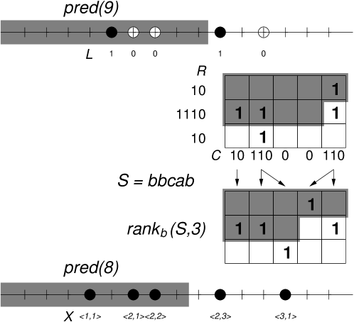
Figure 1: Illustration of the lower bound technique, moving from a predecessor to a $rank$ query, and of the upper bound technique, moving from the $rank$ query to a predecessor query.

Example

Fig. 1 illustrates the technique on a universe of size $u=n\times\sigma=5\times 3=15$, the set $\{5,6,7,10,12\}$ of $n=5$ points black or white, and the query $pred(9)$, which must return the color of the 3rd point. The bitmap $L$ indicates the colors of the points. The top matrix is obtained by taking the first, second, and third ($\sigma=3$) segments of length $n=5$ from the universe, and identifying points with 1-bits (the omitted cells are 0-bits). Bitmaps $R$ and $C$ count the number of 1s in rows and columns, respectively. Bitmap $C$ is used to map the matrix into a new one below it, with exactly one point per column. Then the predecessor query is mapped to the matrix, and spans several whole rows (only 1 in this example) and one partial row. The 1s in whole rows (1 in total) are counted using $R$, whereas those in the partially covered row are counted with a $rank_{b}(S,3)=2$ query on the string $S=bbcab$ represented by the mapped matrix. Then we obtain the desired 3 (3rd point), and $L[3]=0$ is the color. Ignore for now the last line in the figure. $\Box$

Theorem 1

Given a data structure that supports $rank$ queries on strings of length $n$ over alphabet $[1,\sigma]$, in time $t(n,\sigma)$ and using $s(n,\sigma)$ bits of space, we can solve the colored predecessor problem for $n$ integers from universe $[1,n\sigma]$ in time $t(n,\sigma)+O(1)$ using a data structure that occupies $s(n,\sigma)+O(n+\sigma)$ bits.

By the reduction above we get that any lower bound for predecessor search for $n$ keys over a universe of size $n\sigma$ must also apply to $rank$ queries on sequences of length $n$ over alphabet of size $\sigma$. In our case, if we aim at using $n\cdot w^{O(1)}$ bits of space for the $rank$ data structure, and allow any $\sigma\leq n\cdot w^{O(1)}$, this lower bound (branch 2 [Pătraşcu and Thorup (2006)]) is $\Omega\left(\lg\frac{\ell-\lg n}{\lg(s/n)+\lg w}\right)=\Omega\left(\lg\frac{\lg\sigma}{\lg w}\right)$.

Theorem 2

Any data structure that uses $n\cdot w^{O(1)}$ space to represent a sequence of length $n$ over alphabet $[1,\sigma]$, for any $\sigma\leq n\cdot w^{O(1)}$, must use time $\Omega\left(\lg\frac{\lg\sigma}{\lg w}\right)$ to answer $rank$ queries.

For larger $\sigma$, the space of our representation is dominated by the $O(\sigma)$ bits of structure $R$, so the lower bound becomes $\Omega\left(\lg\frac{\lg\sigma}{\lg(\sigma/n)}\right)$, which worsens (decreases) as $\sigma$ grows from $n\cdot w^{\omega(1)}$, and becomes completely useless for $\sigma=n^{1+\Omega(1)}$. However, since the time for $rank$ is monotonic in $\sigma$, we still have the lower bound $\Omega\left(\lg\frac{\lg n}{\lg w}\right)$ when $\sigma>n$; thus a general lower bound is $\Omega\left(\lg\frac{\lg\min(\sigma,n)}{\lg w}\right)$ time. For simplicity we have focused in the most interesting case.

Assume to simplify that $w=\Theta(\lg n)$. The lower bound of Theorem 2 is trivial for small $\lg\sigma=O(\lg\lg n)$ (i.e., $\sigma=O(\mathrm{polylog}~{}n)$), where constant-time solutions for rank exist that require only $nH_{0}(S)+o(n)$ bits [Ferragina et al. (2007)]. On the other hand, if $\sigma$ is sufficiently large, $\lg\sigma=(\lg\lg n)^{1+\Omega(1)}$, the lower bound becomes simply $\Omega(\lg\lg\sigma)$, where it is matched by known compressed solutions requiring as little as $nH_{0}(S)+o(nH_{0}(S))+o(n)$ [Barbay et al. (2012)] or $nH_{k}(S)+o(n\lg\sigma)$ [Grossi et al. (2010)] bits.

The range where this lower bound has not yet been matched is $\omega(\lg\lg n)=\lg\sigma=(\lg\lg n)^{1+o(1)}$. It is also unmatched when $\lg n=o(w)$. The next section presents a new matching upper bound.

3 Optimal Upper Bound for Rank

We now show a matching upper bound with optimal time and space $O(n\lg\sigma)$ bits. In the next sections we make the space succinct and even compressed.

We reduce the problem to predecessor search and then use a convenient solution for that problem. The idea is simply to represent the string $S[1,n]$ over alphabet $[1,\sigma]$ as a matrix of $\sigma$ rows and $n$ columns, and regard each $S[c]$ as a point $(S[c],c)$. Then we represent the matrix as the set of $n$ points $\{(S[c]-1)\cdot n+c,~{}c\in[1,n]\}$ over the one-dimensional universe $[1,n\sigma]$, which is roughly the inverse of the transform used in the previous section. We also store in an array $X[1,n]$ the pairs $\langle r,rank_{r}(S,c)\rangle$, where $r=S[c]$, for the point corresponding to each column $c$ in the set. Those pairs are stored in row-major order in $X$, that is, by increasing point value $(r-1)\cdot n+c$.

To query $rank_{r}(S,c)$ we compute the predecessor of $(r-1)\cdot n+c$, which gives us its position $p$ in $X$. If $X[p]$ is of the form $\langle r,v\rangle$, for some $v$, this means that there are points in row $r$ and columns $[1,c]$ of the matrix, and thus there are occurrences of $r$ in $S[1,c]$. Moreover, $v=rank_{r}(S,c)$ is the value we must return. Otherwise, there are no points in row $r$ and columns $[1,c]$ (i.e., our predecessor query returned a point from a previous row), and thus there are no occurrences of $r$ in $S[1,c]$. Thus we return zero.

Example

Fig. 1 also illustrates the upper-bound technique on string $S=bbcab$, of length $n=5$ over an alphabet of size $\sigma=3$. It corresponds to the lower matrix in the figure, which is read row-wise and the 1s are written as $n=5$ points in a universe of size $n\sigma=15$. To each point we associate the row it comes from and its rank in the row, in array $X$. Now the query $rank_{b}(S,3)$ is converted into query $pred(8)=3$ ($8=5\times 1+3$). This yields $X[3]=\langle 2,2\rangle$, the first 2 indicating that there are $b$s up to position 3 in $S$ ($b$ is the 2nd alphabet symbol), and the second 2 indicating that there are 2 $b$s in the range, so the answer is 2. Instead, a query like $rank_{c}(S,2)$ would be translated into $pred(12)=4$ ($12=5\times 2+2$). This yields $X[4]=\langle 2,3\rangle$. Since the first component is not 3, there are no $c$s up to position 2 in $S$ and the answer is zero. $\Box$

This solution requires $n\lg\sigma+n\lg n$ bits for the pairs of $X$, on top of the space of the predecessor structure. If $\sigma\leq n$ we can reduce this extra space to $2n\lg\sigma$ by storing the pairs $\langle r,rank_{r}(S,c)\rangle$ in a different way. We virtually cut the string into chunks of length $\sigma$, and store the pair as $\langle r,rank_{r}(S,c)-rank_{r}(S,c-(c~{}\mathrm{mod}~{}\sigma))\rangle$, that is, we only store the number of occurrences of $c$ from the beginning of the current chunk. Such a pair requires $2\lg\sigma$ bits. The rest of the $rank_{r}$ information, that is, up to the beginning of the chunk, is obtained in constant time and $O(n)$ bits using the reduction to chunks of GMR06: They store a bitmap $A[1,2n]$ where the matrix is traversed row-wise and we append to $A$ a 1 for each 1 found in the matrix and a 0 each time we move to the next chunk (so we append $n/\sigma$ 0s per row). Then the remaining information for $rank_{r}(S,c)$ is $rank_{r}(S,c-(c~{}\mathrm{mod}~{}\sigma))=select_{0}(A,p_{1})-select_{0}(A,p_{0})-\lfloor c/\sigma\rfloor$, where $p_{0}=(r-1)\cdot n/\sigma$ is the number of chunks in previous rows and $p_{1}=p_{0}+\lfloor c/\sigma\rfloor$ is the number of chunks preceding the current one (we have simplified the formulas by assuming $\sigma$ divides $n$). The $select_{0}(A,\cdot)$ operations map chunk numbers to positions in $A$, and the final formula counts the number of 1s in between.

Theorem 3

Given a solution for predecessor search on a set of $n$ keys chosen from a universe of size $u$, that occupies space $s(n,u)$ and answers in time $t(n,u)$, there exists a solution for $rank$ queries on a sequence of length $n$ over an alphabet $[1,\sigma]$ that runs in time $t(n,n\sigma)+O(1)$ and occupies $s(n,n\sigma)+O(n\lg\sigma)$ bits.

In the extended version of their article, PT08 give an upper bound matching the lower bound of branch 2 and using $O(n\lg u)$ bits for $n$ elements over a universe $[1,u]$. In Appendix A we show that the same time can be achieved with space $O(n\lg(u/n))$, which is not surprising (they have given hints, actually) but we opt for completeness. By using this predecessor data structure, the following result is immediate.

Theorem 4

A string $S[1,n]$ over alphabet $[1,\sigma]$ can be represented using $O(n\lg\sigma)$ bits, so that operation $rank$ is solved in time $O\left(\lg\frac{\lg\sigma}{\lg w}\right)$.

Note that, within $O(n\lg\sigma)$ bits, operations $access$ and $select$ can also be solved in constant time: we can add a plain representation of $A$ to have constant-time $access$, plus a succinct representation [Golynski et al. (2006)] that supports constant-time $select$, adding $2n\lg\sigma+o(n\lg\sigma)$ bits in total.

When $\sigma>n$, we can add a perfect hash function mapping $[1,\sigma]$ to the (at most) $n$ symbols actually occurring in $S$, in constant time, and then $S[1,n]$ can be built over the mapped alphabet of size at most $n$. The hash function can be implemented as an array of $n\lg\sigma$ bits listing the symbols that do appear in $S$ plus $O(n\lg\lg(\sigma/n))$ bits for a mmphf to map from $[1,\sigma]$ to the array [Belazzougui et al. (2009)]. Therefore, in this case we obtain the improved time $O\left(\lg\frac{\lg n}{\lg w}\right)$.

4 Using Succinct Space

We design a sequence representation using $n\lg\sigma+o(n\lg\sigma)$ bits (i.e., succinct) that answers $access$ and $select$ queries in almost-constant time, and $rank$ in time $O\left(\lg\frac{\lg\sigma}{\lg w}\right)$. This is done in two phases: a constant-time solution for $\sigma=w^{O(1)}$, and then a solution for general alphabets.

4.1 Succinct Representation for Small Alphabets

Using multiary wavelet trees [Ferragina et al. (2007), Golynski et al. (2008)] we can obtain succinct space and $O\left(1+\frac{\lg\sigma}{\lg\lg n}\right)$ time for $access$, $select$ and $rank$. This is constant for $\lg\sigma=O(\lg\lg n)$. We start by extending this result to the case $\lg\sigma=O(\lg w)$, as a base case for handling larger alphabets thereafter. More precisely, we prove the following result.

Theorem 5

A string $S[1,n]$ over alphabet $[1,\sigma]$, $\sigma\leq n$, can be represented using $n\lg\sigma+o(n)$ bits so that operations $access$, $select$ and $rank$ can be solved in time $O\left(1+\frac{\lg\sigma}{\lg w}\right)$.

A multiary wavelet tree for $S[1,n]$ divides, at the root node $v$, the alphabet $[1,\sigma]$ into $r$ contiguous regions of the same size. A sequence $R_{v}[1,n]$ recording the region each symbol belongs to is stored at the root node $v$ (note $R_{v}$ is a sequence over alphabet $[1,r]$). This node has $r$ children, each handling the subsequence of $S$ formed by the symbols belonging to a given region. The children are decomposed recursively, thus the wavelet tree has height $h=\lceil\lg_{r}\sigma\rceil$. Queries $access$, $select$ and $rank$ on sequence $S[1,n]$ are carried out via $O(\lg_{r}\sigma)$ similar queries on the sequences $R_{v}$ stored at wavelet tree nodes [Grossi et al. (2003)]. By choosing $r$ such that $\lg r=\Theta(\lg\lg n)$, it turns out that the operations on the sequences $R_{v}$ can be carried out in constant time, and thus the cost of the operations on the original sequence $S$ is $O\left(1+\frac{\lg\sigma}{\lg\lg n}\right)$ [Ferragina et al. (2007)]. GRR08 show how to retain these time complexities within only $n\lg\sigma+o(n)$ bits of space.

In order to achieve time $O\left(1+\frac{\lg\sigma}{\lg w}\right)$, we need to handle in constant time the operations over alphabets of size $r=w^{\beta}$, for some $0<\beta<1$, so that $\lg r=\Theta(\lg w)$. This time we cannot resort to universal tables of size $o(n)$, but rather must use bit manipulation on the RAM model. The description of bit-parallel operations is rather technical; readers interested only in the result (which is needed afterwards) can skip to Section 4.2.

The sequence $R_{v}[1,n]$ is stored as the concatenation of $n$ fields of length $\ell=\lceil\lg r\rceil$, into consecutive machine words. Thus achieving constant-time $access$ is trivial: To access $R_{v}[i]$ we simply extract the corresponding bits, from the $(1+(i-1)\cdot\ell)$-th to the $(i\cdot\ell)$-th, from one or two consecutive machine words, using bit shifts and masking.

Operations $rank$ and $select$ are more complex. We will proceed by cutting the sequence $R_{v}$ into blocks of length $b=\Theta(w^{\alpha}/\ell)$ symbols, for some $\beta<\alpha<1$. First we show how, given a block number $i$ and a symbol $a$, we extract from $R[1,b]=R_{v}[(i-1)\cdot b+1,i\cdot b]$ a bitmap that marks the values $R[j]=a$. Then we use this result to achieve constant-time $rank$ queries. Next, we show how to solve predecessor queries in constant time, for several fields of length $\lg w$ bits fitting in a machine word. Finally, we use this result to obtain constant-time $select$ queries. In the following, we will sometimes write bit-vector constants; in those, bits are written right-to-left, that is, the rightmost bit is that at the bitmap position 1.

Projecting a block

Given sequence $R[1,b]=R_{v}[1+(i-1)\cdot b,i\cdot b]$, which is of bit length $b\cdot\ell=\Theta(w^{\alpha})=o(w)$, and given $a\in[1,r]$, we extract $B[1,b\cdot\ell]$ such that $B[j\cdot\ell]=1$ iff $R[j]=a$. To do so, we first compute $X=a\cdot(0^{\ell-1}1)^{b}$. This creates $b$ copies of $a$ within $\ell$-bit long fields. Second, we compute $Y=R~{}\textsc{xor}~{}X$, which will have zeroed fields at the positions $j$ where $R[j]=a$. To identify those fields, we compute $Z=(10^{\ell-1})^{b}-Y$, which will have a 1 at the highest bit of the zeroed fields in $Y$. Finally, $B=Z~{}\textsc{and}~{}(10^{\ell-1})^{b}$ isolates those leading bits.

Constant-time rank queries

We now describe how we can do rank queries in constant time for $R_{v}[1,n]$. Our solution follows that of Mun96. We choose a superblock size $s=w^{2}$ and a block size $b=(\sqrt{w}-1)/\ell$. For each $a\in[1,r]$, we store the accumulated values per superblock, $rank_{a}(R_{v},i\cdot s)$ for all $1\leq i\leq n/s$. We also store the within-superblock accumulated values per block, $rank_{a}(R_{v},i\cdot b)-rank_{a}(R_{v},\lfloor(i\cdot b)/s\rfloor\cdot s)$, for $1\leq i\leq n/b$. Both arrays of counters require, over all symbols, $r((n/s)\cdot w+(n/b)\cdot\lg s)=O(nw^{\beta}(\lg w)^{2}/\sqrt{w})$ bits. Added over the $O\left(\frac{\lg\sigma}{\lg w}\right)$ wavelet tree levels, the space required is $O(n\lg\sigma\lg w/w^{1/2-\beta})$ bits. This is $o(n\lg\sigma)$ for any $\beta<1/2$.

To solve a query $rank_{a}(R_{v},i)$, we need to add up three values: $(i)$ the superblock accumulator at position $\lfloor i/s\rfloor$, $(ii)$ the block accumulator at position $\lfloor i/b\rfloor$, $(iii)$, the bits set at $B[1,(i~{}\mathrm{mod}~{}b)\cdot\ell]$, where $B$ corresponds to the values equal to $a$ in $R_{v}[\lfloor i/b\rfloor\cdot b+1,\lfloor i/b\rfloor\cdot b+b]$. We have just shown how to extract $B[1,b\cdot\ell]$ from $R_{v}$, so we count the number of bits set in $C=B~{}\textsc{and}~{}1^{(i~{}\mathrm{mod}~{}b)\cdot\ell}$.

This counting is known as a popcount operation. Given a bit block $C$ of length $b\ell=\sqrt{w}-1$, with bits possibly set at positions multiple of $\ell$, we popcount it using the following steps:

1. We first duplicate the block $b$ times into $b$ fields. That is, we compute $X=C\cdot(0^{b\ell-1}1)^{b}$.

2. We now isolate a different bit in each different field. This is done with $Y=X~{}\textsc{and}~{}(0^{b\ell}10^{\ell-1})^{b}$. This will isolate the $i$th aligned bit in field $i$.

3. We now sum up all those isolated bits using the multiplication $Z=Y\cdot(0^{b\ell+\ell-1}1)^{b}$. The result of the popcount operation lies at the bits $Z[b^{2}\ell,b^{2}\ell+\lg b-1]$.

4. We finally extract the result as $c=(Z\gg(b^{2}\ell-1))~{}\textsc{and}~{}(1^{\lg b})$.

Constant-time select queries

We now describe how we can do $select$ queries in constant time for $R_{v}[1,n]$. Our solution follows that of Cla96. For each $a\in[1,r]$, consider the virtual bitmap $B_{a}[1,n]$ so that $B_{a}[j]=1$ iff $R_{v}[j]=a$. We choose a superblock size $s=w^{2}$ and a block size $b=w^{1/3}/(2\lg r)$. Superblocks contain $s$ 1-bits and are of variable length. They are called dense if their length is at most $w^{4}$, and sparse otherwise. We store all the positions of the 1s in sparse superblocks, which requires $O(n/w)$ bits of space as there are at most $n/w^{4}$ sparse superblocks. For dense superblocks we only store their starting position in $R_{v}$ and a pointer to a memory area. Both pointers require $O(n/w)$ bits since there are at most $n/w^{2}$ superblocks.

We divide the dense superblocks into blocks of $b$ 1s. Blocks are called dense if their length is at most $w^{2/3}$, and sparse otherwise. We store all the positions of the 1s in sparse blocks. Since each position requires only $\lg(w^{4})$ as it is within a dense superblock, and there are at most $n/w^{2/3}$ sparse blocks, the total space for sparse blocks is $O((n/w^{2/3})b\lg w)=O(n/w^{1/3})$ bits. For dense blocks we store only their starting position within their dense superblock, which requires $O((n/b)\lg w)=O(n(\lg w)^{2}/w^{1/3})$ bits.

The space, added over the $r$ symbols, is $O(rn(\lg w)^{2}/w^{1/3})=O(n(\lg w)^{2}/w^{1/3-\beta})$. Summing for $O\left(\frac{\lg\sigma}{\lg w}\right)$ wavelet tree levels, the total space is $O(n\lg\sigma\lg w/w^{1/3-\beta})$ bits. This is $o(n\lg\sigma)$ for any $\beta<1/3$.

In order to compute a $select_{a}(R_{v},j)$ query, we use the data structures for virtual bitmap $B_{a}[1,n]$. If $\lfloor j/s\rfloor$ is a sparse superblock, then the answer is readily stored. If it is a dense superblock, we only know its starting position and the offset $o=j-(j~{}\mathrm{mod}~{}s)$ of the query within its superblock. Now, if $\lfloor o/b\rfloor$ is a sparse block in its superblock, then the answer (which must be added to the starting position of the superblock) is readily stored. If it is a dense block, we only know its starting position in $R_{v}$ (and in $B_{a}$), but now we only have to complete the search within an area of length $b=O(w^{1/3}/\lg w)$ in $B_{a}$. We have showed how to extract a chunk $B[1,b\cdot\ell]$ from $R_{v}$, so that $B[i\cdot\ell]=B_{a}[i]$. Now we detail how we complete a $select$ query within a chunk of length $b\cdot\ell=O(w^{1/3})$ for the remaining $j^{\prime}=j-(j~{}\mathrm{mod}~{}b)$ bits. This is based on doing about $w^{1/3}$ parallel popcount operations on about $w^{1/3}$ bit blocks. We proceed as follows:

1. Duplicate $B$ into $b$ superfields with $X=B\cdot(0^{k-1}1)^{b}$, where $k=2b^{2}\ell$ is the superfield size.

2. Compute $Y=X~{}\textsc{and}~{}(0^{k-b\ell}1^{b\ell})\ldots(0^{k-2\ell}1^{2\ell})(0^{k-\ell}1^{\ell})$. This operation will keep only the first $i$ aligned bits in superfield $i$.

3. Do popcount in parallel on all superfields using the algorithm described in Section 4.1. Note that each superfield will have capacity $k=2b^{2}\ell$, but only the first $b\ell$ bits in it are set, and the alignment is $\ell$. Thus the popcount operation will have enough available space in each superblock to operate.

4. Let $Z$ contain all the partial counts for all the prefixes of $B$. We need the position in $Z$ of the first count equal to $j^{\prime}$. We use the same projecting method described in Section 4.1 to spot the superfields equal to $j^{\prime}$ (the only difference is that superfields are much wider than $\lg w$, namely of width $\ell=k$, but still all fits in a machine word). This method returns a word $W[1,2b^{3}\ell]$ such that $W[k\cdot i]=1$ iff the $i$th superfield of $Z$ is equal to $j^{\prime}$.

5. Isolate the least significant bit of $W$ with $V=W~{}\textsc{and}~{}(W~{}\textsc{xor}~{}(W-1))$.

6. The final answer to $select_{1}(B,j^{\prime})$ is the position of the only 1 in $V$, divided by $k$. This is easily computed by using mmphfs over the set $\{2^{ki},~{}1\leq i\leq b\}$. Existing data structures [Belazzougui et al. (2009)] take constant time and $O(b\lg w)=O(w)$ bits. Such a data structure is universal and requires the same space as systemwide pointers.

Space analysis

We choose $r=w^{\beta}$ to be a power of 2, $r=2^{\ell}$. This is always possible because it is equivalent to finding an integer $\ell=\beta\lg w$, where we can choose any constant $0<\beta<1/3$ and any $\ell=\Theta(\lg w)$ (e.g., one solution is $\beta=\lfloor\frac{\lg w}{4}\rfloor/\lg w$, $\ell=\lfloor\lg w/4\rfloor$, and $r=2^{\lfloor\lg w/4\rfloor}\approx w^{1/4}$). In this case the wavelet tree simply stores, at level $l$, the bits $(l-1)\cdot\ell+1$ to $l\cdot\ell$ of the binary descriptions of the symbols of $S$. The wavelet tree has height $h=\lceil\lg_{r}\sigma\rceil=\lceil(\lg\sigma)/\ell\rceil$, so it will store sequences of symbols of $\ell=\lg r$ bits in each of the $h$ levels except in the first, where it will store a sequence of symbols of $\lceil\lg\sigma\rceil-(h-1)\ell\leq\ell$ bits. The total adds up to $n\lceil\lg\sigma\rceil$ bits.

This is not fully satisfactory when $\sigma$ is not a power of two. In this case we proceed as follows. We choose an integer $y=\lg\sigma-\Theta(\lg\lg n)$ as the number of bits of the representation that will be stored integrally, just as explained. The other $x=\lg\sigma-y$ bits (where $x$ is not an integer) will be represented as symbols over alphabet $[1,\sigma_{0}]=[1,\lceil 2^{x}\rceil]=[1,\lceil\sigma/2^{y}\rceil]$. By construction, $\sigma_{0}=\lg^{\Theta(1)}n$, thus we can represent the sequence of $x$ highest bits (i.e., the numbers $\lceil S[i]/2^{y}\rceil$) using the space-efficient wavelet tree of GRR08. This will take $n\lg\sigma_{0}+o(n)$ bits and support $access$, $select$ and $rank$ in constant time, and will act as the root level of our whole wavelet tree. For each value $c\in[1,\sigma_{0}]$ we will store, as a child of that root, a separate wavelet tree handling the subsequence of positions $i$ such that $\lceil S[i]/2^{y}\rceil=c$. These wavelet trees will handle the $y$ lower bits of the sequence with the technique of the previous paragraph, which will take $ny$ bits and solve the three queries in $O\left(1+\frac{y}{\lg w}\right)$ time. Adding up the spaces we get $n\lg\sigma_{0}+ny+o(n)<n(\lg(1+\sigma/2^{y})+y+o(1))=n(\lg(\sigma+2^{y})+o(1))=n(\lg(\sigma(1+1/\lg^{\Theta(1)}n))+o(1))\leq n(\lg\sigma+1/\lg^{\Theta(1)}n+o(1))=n\lg\sigma+o(n)$.

To this space we must add the $o(n\lg\sigma)$ bits of the extra structures to support $rank$ and $select$ on the wavelet tree levels. The special level using less than $\ell$ bits can use the same $\alpha$ value of the next levels without trouble (actually the redundancy may be lower since more symbols can be packed in the blocks).

In order to further reduce the redundancy to $o(n)$ bits, we use the scheme we have described only for $w>\lg^{d}n$, for some constant $d$ to be defined soon. For smaller $w$, we directly use the scheme of GRR08, which uses $n\lg\sigma+o(n)$ bits and solves all the operations in time $O\left(1+\frac{\lg\sigma}{\lg\lg n}\right)=O\left(1+\frac{\lg\sigma}{\lg w}\right)$. For the larger $w$ case, and choosing our example $\beta\leq 1/4$, our redundancy is of the form $O(n\lg\sigma\cdot(\lg w/w^{1/3-\beta}))=O(n\lg n\cdot(d\lg\lg n/(\lg n)^{d/12}))$, which is made $o(n)$ by choosing any $d>12$ (a smaller $d$ can be chosen if a smaller $\beta$ is used).

Finally, we have the space redundancy of the wavelet tree pointers. On binary wavelet trees this is easily solved by concatenating all the bitmaps [Mäkinen and Navarro (2007)]. This technique can be extended to $r$-ary wavelet trees, but in this case a simpler solution is as follows. As the wavelet tree has a perfect $r$-ary structure, we deploy its nodes levelwise in memory. For each level, we concatenate all the sequences of the nodes, read left-to-right, into a large sequence of at most $n$ symbols. Then the node position we want at each level can be algebraically computed from that of the previous or next level, whereas its starting positions in the concatenation of sequences can be marked in a bitmap of length $n$, which will have at most $r^{j}$ 1s for the level $j$ of the wavelet tree. Using the representation of RRR07 for this bitmap, the space is $O(r^{j}\lg(n/r^{j}))+o(n)$ bits. Thus the space is dominated by the last level, which has $r^{j}=\sigma/w^{\beta}\leq n/w^{\beta}$ 1s, giving overall space $O(n\lg w/w^{\beta})+o(n)=o(n)$ bits. Then any pointer can be retrieved with a constant-time $select$ operation on the bitmap of its level.

4.2 Succinct Representation for Larger Alphabets

We now assume $\lg\sigma=\omega(\lg w)$ and develop fast succinct solutions for these larger alphabets. We build on the solution of GMR06. They first cut $S$ into chunks of length $\sigma$. With the bitvector $A[1,2n]$ described in Section 3 they reduce all the queries, in constant time, to within a chunk. For each chunk they store a bitmap $X[1,2\sigma]$ where the number of occurrences of each symbol $a\in[1,\sigma]$ in the chunk, $n_{a}$, is concatenated in unary, $X=1^{n_{1}}01^{n_{2}}0\ldots 1^{n_{\sigma}}0$. Now they introduce two complementary solutions.

Constant-time select

The first one stores, for each consecutive symbol $a\in[1,\sigma]$, the chunk positions where it appears, in increasing order. Let $\pi$ be the resulting permutation, which is stored with the representation of MRRR03. This requires $\sigma\lg\sigma(1+1/f(n,\sigma))$ bits and computes any $\pi(i)$ in constant time and any $\pi^{-1}(j)$ in time $O(f(n,\sigma))$, for any $f(n,\sigma)\geq 1$. With this representation they solve, within the chunk, $select_{a}(i)=\pi(select_{0}(X,a-1)-(a-1)+i)$ in constant time and $access(i)=1+rank_{0}(select_{1}(X,\pi^{-1}(i)))$ in time $O(f(n,\sigma))$.

For $rank_{a}(i)$, they basically carry out a predecessor search within the interval of $\pi$ that corresponds to $a$: $[select_{0}(X,a-1)-(a-1)+1,select_{0}(X,a)-a]$. They have a sampled predecessor structure with one value out of $\lg\sigma$, which takes just $O(\sigma)$ bits. With this structure they reduce the interval to size $\lg\sigma$, and a binary search completes the process, within overall time $O(\lg\lg\sigma)$.

To achieve optimal time, we sample one value out of $\frac{\lg\sigma}{\lg w}$. We build the predecessor data structures of PT08 mentioned in Section 3. Over all the symbols of the chunk, these structures take $O\left(\left(n/\frac{\lg\sigma}{\lg w}\right)\lg\sigma\right)=O(n\lg w)=o(n\lg\sigma)$ bits (as we assumed $\lg\sigma=\omega(\lg w)$). The predecessor structures take time $O\left(\lg\frac{\lg\sigma}{\lg w}\right)$ (see Theorem 14 in Appendix A). The final binary search time also takes time $O\left(\lg\frac{\lg\sigma}{\lg w}\right)$.

Constant-time access

This time we use the structure of Munro et al. on $\pi^{-1}$, so we compute any $\pi^{-1}(j)$ in constant time and any $\pi(i)$ in time $O(f(n,\sigma))$. Thus we get $access$ in constant time and $select$ in time $O(f(n,\sigma))$.

Now the binary search of $rank$ needs to compute values of $\pi$, which is not anymore constant time. This is why GMR06 obtained time slightly over $\lg\lg\sigma$ time for $rank$ in this case. We instead set the sampling step to $\left(\frac{\lg\sigma}{\lg w}\right)^{\frac{1}{f(n,\sigma)}}$. The predecessor structures on the sampled values still answer in time $O\left(\lg\frac{\lg\sigma}{\lg w}\right)$, but they take $O\left(\left(n/\left(\frac{\lg\sigma}{\lg w}\right)^{\frac{1}{f(n,\sigma)}}\right)\lg\sigma\right)$ bits of space. This is $o(n\lg\sigma)$ provided $f(n,\sigma)=o\left(\lg\frac{\lg\sigma}{\lg w}\right)$. On the other hand, the time for the binary search is $O\left(\frac{f(n,\sigma)}{f(n,\sigma)}\lg\frac{\lg\sigma}{\lg w}\right)$, as desired.

The following theorem, which improves upon the result of GMR06 (not only as a consequence of a higher low-order space term), summarizes our result. Note that we do not mention the limit $f(n,\sigma)=o\left(\lg\frac{\lg\sigma}{\lg w}\right)$, as if a larger $f(n,\sigma)$ is desired we can always use a smaller one (and be faster). We also omit the condition $\lg\sigma=\omega(\lg w)$ because otherwise the result also holds by Theorem 5.

Theorem 6

A string $S[1,n]$ over alphabet $[1,\sigma]$, $\sigma\leq n$, can be represented using $n\lg\sigma+o(n\lg\sigma)$ bits, so that, given any function $f(n,\sigma)=\omega(1)$, $(i)$ operations $access$ and $select$ can be solved in time $O(1)$ and $O(f(n,\sigma))$, or vice versa, and $(ii)$ $rank$ can be solved in time $O\left(\lg\frac{\lg\sigma}{\lg w}\right)$.

Note that we can partition into chunks only of $\sigma\leq n$. If $\sigma=o(n\lg n)$ we can still apply the same scheme using a single chunk, and the space overhead for having $\sigma>n$ will be $O(\sigma)=o(n\lg\sigma)$. For larger $\sigma$, however, we must use a mechanism like the one used at the end of Section 3, mapping $[1,\sigma]$ to $[1,n]$. However, this adds at least $n\lg\sigma$ bits to the space, and thus the space is not succinct anymore, unless $\sigma$ is much larger, $\lg\sigma=\omega(\lg n)$, so that the space of the mapping array dominates. For simplicity we will consider only the case $\sigma\leq n$ in the rest of the article.

5 Compressing the Space

Now we compress the space of the succinct solutions of the previous sections. First we achieve zeroth-order compression (of the data and the redundancy) by using an existing compression booster [Barbay et al. (2012)]. Second, we reach high-order compression by designing an index that operates over a compressed representation [Ferragina and Venturini (2007)] and simulates the working of a succinct data structure of the previous section.

5.1 Zero-order Compression

[Thm. 2]BCGNN12 showed how, given a sequence representation $\mathcal{R}$ using $n\lg\sigma(1+r(n,\lg\sigma))+o(n)$ bits, where $r(n,\lg\sigma)=O(1)$ is nonincreasing with $\sigma$, its times for $access$, $select$ and $rank$ can be maintained while reducing its space to $nH_{0}(S)(1+r(n,\Theta(\lg\lg n))+o(n)$ bits. This can be done even if $\mathcal{R}$ works only for $\sigma\geq\lg^{c}n$ for some constant $c$.

The technique separates the symbols according to their frequencies into $\lg^{2}n$ classes. The sequence of classes is represented using a multiary wavelet tree [Ferragina et al. (2007)], and the subsequences of the symbols of each class are represented with an instance of $\mathcal{R}$ if the local alphabet size is $\sigma^{\prime}\geq\lg^{c}n$, or with a multiary wavelet tree otherwise. Hence the global per-bit redundancy can be upper bounded by $r(n,c\lg\lg n)$ and it is shown that the total number of bits represented is $nH_{0}(S)+O(n/\lg n)$.

We can use this technique to compress the space of our succinct representations. By using Theorem 5 as our structure $\mathcal{R}$, where we can use $r(n,\lg\sigma)=0$, we improve upon FMMN07 and GRR08.

Theorem 7

A string $S[1,n]$ over alphabet $[1,\sigma]$, $\sigma\leq n$, can be represented using $nH_{0}(S)+o(n)$ bits so that operations $access$, $select$ and $rank$ can be solved in time $O\left(1+\frac{\lg\sigma}{\lg w}\right)$.

To obtain better times when $\lg\sigma=\omega(\lg w)$, we use Theorem 6 as our structure $\mathcal{R}$. A technical problem is that BCGNN12 apply $\mathcal{R}$ over smaller alphabets $[1,\sigma^{\prime}]$, and thus in Theorem 6 we would sample one position out of $\frac{\lg\sigma^{\prime}}{\lg w}$, obtaining $O\left(\lg\frac{\lg\sigma^{\prime}}{\lg w}\right)$ time and $O\left(n\lg\sigma^{\prime}\frac{\lg w}{\lg\sigma^{\prime}}\right)$ bits of space, which is $o(n\lg\sigma^{\prime})$ only if $\lg\sigma^{\prime}=\omega(\lg w)$ (this is why we have used Theorem 6 only in that case). To handle this problem, we will use a sampling of size $\frac{\lg\sigma}{\lg w}$ (or $\left(\frac{\lg\sigma}{\lg w}\right)^{\frac{1}{f(n,\sigma)}}$ in the case of constant-time $access$), even if the alphabet of the local sequence is of size $\sigma^{\prime}$. As a consequence, the redundancy will be $O(n\lg\sigma^{\prime}\,\frac{\lg w}{\lg\sigma})=o(n\lg\sigma^{\prime})$ and the time for $rank$ will stay $O\left(\lg\frac{\lg\sigma}{\lg w}\right)$ (instead of $O\left(\lg\frac{\lg\sigma^{\prime}}{\lg w}\right)$). Similarly, we always use sampling rate $f(n,\sigma)$ instead of $f(n,\sigma^{\prime})$. Therefore our redundancy is $r(n,\lg\sigma)=O\left(\frac{\lg w}{\lg\sigma}+\frac{1}{f(n,\sigma)}\right)$, which is $o(1)$ if $\lg\sigma=\omega(\lg w)$.

Still, in the first levels where $\sigma^{\prime}=O(1)$, the redundancy of Theorem 6 contains space terms of the form $O(n)$ that would not be $o(n\lg\sigma^{\prime})$. To avoid this, we will use Theorem 5 up to $\frac{\lg\sigma^{\prime}}{\lg w}\leq 1$, where all times are constant, and the variant just described for larger $\sigma^{\prime}$. The result is an improvement over BCGNN12 (again, we do not mention the condition $\lg\sigma=\omega(\lg w)$ because otherwise the result holds anyway by Theorem 7).

Theorem 8

A string $S[1,n]$ over alphabet $[1,\sigma]$, $\sigma\leq n$, can be represented using $nH_{0}(S)+o(nH_{0}(S))+o(n)$ bits, so that, given any function $f(n,\sigma)=\omega(1)$, $(i)$ operations $access$ and $select$ can be solved in time $O(1)$ and $O(f(n,\sigma))$, or vice versa, and $(ii)$ $rank$ can be solved in time $O\left(\lg\frac{\lg\sigma}{\lg w}\right)$.

5.2 Self-Indexing

Likewise, we can improve upon the result of BCGNN12 that plugs a zeroth-order compressed sequence representation to obtain a $k$-th order compressed full-text self-index [Barbay et al. (2012), Thm. 5]. This result is not subsumed by that of BN11 because their index, although obtaining better times, uses $O(n)$ extra bits of space. Ours is the best result using only $o(n)(H_{k}(S)+1)$ bits of redundancy. We start with a version for small alphabets.

Theorem 9

Let $S[1,n]$ be a string over alphabet $[1,\sigma]$, $\lg\sigma=O(\lg w)$. Then we can represent $S$ using $nH_{k}(S)+o(n)$ bits, for any $k\leq(\delta\lg_{\sigma}n)-1$ and constant $0<\delta<1$, while supporting the following queries, for any function $f(n)=\omega(1)$: $(i)$ count the number of occurrences of a pattern $P[1,m]$ in $S$, in time $O(m)$; $(ii)$ locate any such occurrence in time $O(f(n)\lg n)$; $(iii)$ extract $S[l,r]$ in time $O(r-l+f(n)\lg n)$.

To obtain this result, we follow the proof of Theorem 5 of BCGNN12. Our zeroth-order compressed structure will be that of our Theorem 7, with constant time for all the operations and space overhead $O(n/\lg^{\gamma}n)=o(n)$ bits, for some $0<\gamma<1$. For operations $(ii)$ and $(iii)$, we sample one text position out of $O(f(n)\lg n)$ in the suffix array to obtain the claimed times.

On general alphabets, we obtain the following result, where once again we only need to prove the case $\lg\sigma=\omega(\lg w)$.

Theorem 10

Let $S[1,n]$ be a string over alphabet $[1,\sigma]$, $\sigma\leq n$. Then we can represent $S$ using $nH_{k}(S)+o(n)(H_{k}(S)+1)$ bits, for any $k\leq(\delta\lg_{\sigma}n)-1$ and constant $0<\delta<1$, while supporting the following queries, for any $f(n,\sigma)=\omega(1)$: $(i)$ count the number of occurrences of a pattern $P[1,m]$ in $S$, in time $O\left(m\lg\frac{\lg\sigma}{\lg w}\right)$; $(ii)$ locate any such occurrence in time $O(f(n,\sigma)\lg n)$; $(iii)$ extract $S[l,r]$ in time $O(r-l+f(n,\sigma)\lg n)$.

Again we follow the proof of Theorem 5 of BCGNN12. First, if $f(n,\sigma)=\omega\left(\lg\frac{\lg\sigma}{\lg w}\right)$, we set it to $f(n,\sigma)=\lg\frac{\lg\sigma}{\lg w}$, to ensure that no operation will be slower than $rank$. Our string structure will be that of Theorem 8 with constant-time $select$, $O(f(n,\sigma))$ time $access$, and $O(nH_{0}(S)(\lg w/\lg\sigma+1/f(n,\lg\sigma))+o(n)$ bits of overhead. BCGNN12 partition the text into strings $S^{i}$, which are represented to their zeroth-order entropy. The main issue is to upper bound the sum of the redundancies over all the strings $S^{i}$ in terms of the total length $n$. More precisely, we need to bound the factor multiplying $|S^{i}|H_{0}(S^{i})$, $O(\lg w/\lg\sigma+1/f(|S^{i}|,\lg\sigma))$, in terms of $n$ and not $|S^{i}|$. However, we can simply use the sampling value $f(n,\sigma)$ for all the strings $S^{i}$ that are represented using Theorem 8, regardless of the length $|S^{i}|$. Then their Theorem 5 can be applied immediatly.

For operations $(ii)$ and $(iii)$, we again sample one out of $O(f(n,\sigma)\lg n)$ text positions in the suffix array, but instead of moving backward in the text using $rank$ and $access$, we move forward using $select$, as in [Sec. 4]BN11, which is constant-time.

5.3 High-order Compression

FV07 showed how a string $S[1,n]$ over alphabet $[1,\sigma]$ can be stored within $nH_{k}(S)+o(n\lg\sigma)$ bits, for any $k=o(\lg_{\sigma}n)$, so that it offers constant-time $access$ to any $O(\lg_{\sigma}n)$ consecutive symbols.

We provide $select$ and $rank$ functionality on top of this representation by adding extra data structures that take $o(n\lg\sigma)$ bits, whenever $\lg\sigma=\omega(\lg w)$. The technique is similar to those used by BHMR11 and GOR10, and we use the terminology of Section 4.2. We divide the text logically into chunks, as with GMR06, and for each chunk we store a mmphf $f_{a}$ for each $a\in[1,\sigma]$. Each $f_{a}$ stores the positions where symbol $a$ occurs in the chunk, so that given the position $i$ of an occurrence of $a$, $f_{a}(i)$ gives $rank_{a}(i)$ within the chunk. All the mmphfs can be stored within $O(n\lg\lg\sigma)=o(n\lg\sigma)$ bits and can be queried in constant time [Belazzougui et al. (2009)]. With array $X$ we can know, given $a$, how many symbols smaller than $a$ are there in the chunk.

Now we have sufficient ingredients to compute $\pi^{-1}$ in constant time: Let $a$ be the $i$th symbol in the chunk (obtained in constant time using Ferragina and Venturini’s structure), then $\pi^{-1}(i)=f_{a}(i)+select_{0}(X,a-1)-(a-1)$. Now we can compute $select$ and $rank$ just as done in the “constant-time $access$” branch of Section 4.2. The resulting theorem improves upon the results of BHMR11 (they did not use mmphfs).

Theorem 11

A string $S[1,n]$ over alphabet $[1,\sigma]$, for $\sigma\leq n$ and $\lg\sigma=\omega(\lg w)$, can be represented using $nH_{k}(S)+o(n\lg\sigma)$ bits for any $k=o(\lg_{\sigma}n)$ so that, given any function $f(n,\sigma)=\omega(1)$, $(i)$ operation $access$ can be solved in constant time, $(ii)$ operation $select$ can be solved in time $O(f(n,\sigma))$, and $(ii)$ operation $rank$ can be solved in time $O\left(\lg\frac{\lg\sigma}{\lg w}\right)$.

To compare with the corresponding result by GOR10, who do use mmphfs to achieve $nH_{k}(S)+O(n\lg\sigma/\lg\lg\sigma)$ bits, $O(1)$ time for $access$ and $O(\lg\lg\sigma)$ time for $select$ and $rank$, we can fix $f(n,\sigma)=\lg\lg\sigma$ to obtain the same redundancy. Then we obtain the same time for operations $access$ and $select$, and improved time for $rank$. Their results, however, hold for any alphabet size, which we do not cover for the case $\lg\sigma=O(\lg w)$. We can, however, improve that branch too, by using any superconstant sampling $g(n,\sigma)^{\frac{1}{f(n,\sigma)}}$, for $\lg g(n,\sigma)=\omega(f(n,\sigma))$. Then the time for $rank$ becomes $O(\frac{f(n,\sigma)}{f(n,\sigma)}\lg g(n,\sigma))$. By using, say, $\lg g(n,\sigma)=f(n,\sigma)^{2}$, we get the following result.

Theorem 12

A string $S[1,n]$ over alphabet $[1,\sigma]$, for $\lg\sigma=O(\lg w)$, can be represented using $nH_{k}(S)+o(n\lg\sigma)$ bits for any $k=o(\lg_{\sigma}n)$ so that, given any function $f(n,\sigma)=\omega(1)$, $(i)$ operation $access$ can be solved in constant time, $(ii)$ operation $select$ can be solved in time $O(f(n,\sigma))$, and $(ii)$ operation $rank$ can be solved in time $O(f^{2}(n,\sigma))$.

This result, while improving that of GOR10, is not necessarily optimal, as no lower bound prevents us from reaching constant time for all the operations. We can achieve time optimality and $k$th order compression for small alphabet sizes, as follows. We build on the representation of FV07. For $k=o(\lg_{\sigma}n)$, they partition the sequence $S[1,n]$ into chunks of $s=\frac{1}{2}\lg_{\sigma}n=\omega(k)$ symbols, and encode the sequence of chunks $S^{\prime}[1,n/s]$ over alphabet $[1,\sigma^{s}]=[1,\sqrt{n}]$ into zeroth-order entropy. This gives $k$th order compression of $S$ and supports constant-time access to any chunk. Now we add, for each $c\in[1,\sigma]$, a bitmap $B_{c}[1,n/s]$ so that $B_{c}[i]=1$ iff chunk $S^{\prime}[i]$ contains an occurrence of symbol $c$. We store in addition a bitmap $C_{c}$ with the number of occurrences, in unary, of $c$ in all the chunks $i$ where $B_{c}[i]=1$. That is, for each $B_{c}[i]=1$, we append $0^{m-1}1$ to $C_{c}$, where $m$ is the number of times $c$ occurs in the chunk $S^{\prime}[i]$. Then we can easily know the number of occurrences of any $c$ in $S^{\prime}[1,i]$ using $select_{1}(C_{c},rank_{1}(B_{c},i))$. With a universal table on the chunks, of size $\sigma^{s+1}\lg s=O(\sqrt{n}\,\mathrm{polylog}(n))=o(n)$, we can complete the computation of any $rank_{c}(S,i)$ in constant time. Similarly, we can determine in which chunk is the $j$th occurrence of any $c$ in $S^{\prime}$, by computing $select_{1}(B_{c},1+rank(C_{c},j))$, and then we can easily complete the calculation of any $select_{c}(S,j)$ with a similar universal table, all in constant time.

Let us consider space now. The $B_{c}$ bitmaps add up to $\sigma n/s$ bits, of which at most $n$ are set. By using the representation of RRR07 we get total space $n\lg\frac{\sigma}{s}+O\left(n+\frac{(\sigma n/s)\lg\lg(\sigma n/s)}{\lg(\sigma n/s)}\right)$ bits, which is $o(n\lg\sigma)$ for any $\sigma=O(\lg^{1+o(1)}n)$ and $\sigma=\omega(1)$. On the other hand, the $C_{c}$ bitmaps add up to length $n$ and require $o(n\lg\sigma)$ bits of space for any $\sigma=\omega(1)$.

For constant $\sigma$, instead, we can represent the $B_{c}$ bitmaps in plain form, using $O(\sigma n/s)=o(n)$ bits, and the $C_{c}$ bitmaps using Raman et al., as they have only $\sigma n/s=O(n/s)$ 1s, and thus their total space is $O(\frac{n\lg s}{s})+o(n)=o(n)$ bits. The same time complexities are maintained.

Theorem 13

A string $S[1,n]$ over alphabet $[1,\sigma]$, for $\sigma=O\left(\lg^{1+o(1)}n\right)$, can be represented using $nH_{k}(S)+o(n\lg\sigma)$ bits for any $k=o(\lg_{\sigma}n)$ so that operations $access$, $select$ and $rank$ can be solved in constant time.

6 Conclusions

This work considerably reduces the gap between upper and lower bounds for sequence representations providing $access$, $select$ and $rank$ queries. Most notably, we give matching lower and upper bounds $\Theta\left(\lg\frac{\lg\sigma}{\lg w}\right)$ for operation $rank$, which was the least developed one in terms of lower bounds. The issue of the space related to this complexity is basically solved as well: we have shown it can be achieved even within compressed space, and it cannot be surpassed within space $O(n\cdot w^{O(1)})$. On the other hand, operations $access$ and $select$ can be solved, within the same compressed space, in almost constant time (i.e., one taking $O(1)$ and the other as close to $O(1)$ as desired but not both reaching it, unless we double the space). Our new compressed representations improve upon most of the previous work.

There are still, however, some intriguing issues that remain unclear, which prevent us from considering this problem completely closed:

1. The lower bounds of Gol09 leave open the door to achieving constant time for $access$ and $select$ simultaneously, with $O(n\lg\sigma\,\frac{\lg\sigma}{w})$ bits of redundancy. That is, both could be constant time with $o(n\lg\sigma)$ redundancy in the interesting case $\lg\sigma=o(w)$. We have achieved this when $\lg\sigma=O(\lg w)$, but it is open whether this is possible in the area $\omega(\lg w)=\lg\sigma=o(w)$. In our solution, this would imply computing $\pi$ and $\pi^{-1}$ in constant time on a permutation using $n\lg n+o(n\lg n)$ bits. A lower bound on the redundancy of permutations in the same paper [Golynski (2009)], $\Omega\left(n\lg n\,\frac{\lg n}{w}\right)$ bits, forbids this for $\lg n=\Theta(w)$ but not for $\lg n=o(w)$. It is an interesting open challenge to achieve this or prove that a stronger lower bound holds.

2. While we can achieve constant-time $select$ and almost-constant time for $access$ (or vice versa), only the second combination is possible within high-order entropy space. Lower bounds on the indexing model [Grossi et al. (2010)] show that this must be the case (at least in the general case where $\lg\sigma=\Theta(w)$) as long as our solution builds on a compressed representation of $S$ supporting constant-time access, as it has been the norm [Barbay et al. (2011), Barbay et al. (2012), Grossi et al. (2010)]. Yet, it is not clear that this is the only way to reach high-order compression.

3. We have achieved high-order compression with almost-constant $access$ and $select$ times, and optimal $rank$ time, but on alphabets of size superpolynomial in $w$. For smaller alphabets, although constant time seems to be possible, we achieved it only for $\sigma=O(\lg^{1+o(1)}n)$. This leaves open the interesting band of alphabet sizes $\lg^{1+\Omega(1)}n=\sigma=w^{O(1)}$, where we have achieved only (any) superconstant time. It is also unclear whether we can obtain $o(n)$ redundancy, instead of $o(n\lg\sigma)$, for alphabets polynomial in $w$, with high-order compression.

Appendix A Upper Bound for Predecessor Search

We describe a data structure that stores a set $S$ of $n$ elements from universe $U=[1,u]$ in $O(n\lg(u/n))$ bits of space, while supporting predecessor queries in time $O(\lg\frac{\lg u-\lg n}{\lg w})$. We first start with a solution that uses $O(n\lg u)$ bits of space. We use a variant of the traditional recursive van Emde Boas solution [Pătraşcu and Thorup (2008)]. Let $\ell\geq\lg u$ be the length of the keys. We choose $\ell$ as the smallest value of the form $\ell=(\lg w-1)\cdot 2^{i}\geq\lg u$, for some integer $i\geq 0$ (note $\ell\leq 2\lg u$). We denote the predecessor data structure that stores a set $S$ of keys of length $\ell$ by $D^{\ell}(S)$. Given an element $x$ the predecessor data structure should return a pair $(y,r)$ where $y$ is the predecessor of $x$ in $S$ (i.e., the maximum value $\leq x$ in $S$) and $r$ is the rank of $y$ in $S$ (i.e., the number of elements of $S$ smaller than or equal to $y$). If the key $x$ has no predecessor in $S$ (i.e., it is smaller than any key in $S$), the query should return $(0,0)$.

We now describe the solution. We partition the set $S$ according to the most significant $\ell/2$ bits. We call $h(x)$ the $\ell/2$ most significant bits of $x$, and $l(x)$ the $\ell/2$ least significant bits of $x$, $x=2^{\ell/2}h(x)+l(x)$.

Let $S_{p}=\{x\in S,h(x)=p\}$ denote the set of all the elements $x$ such that $h(x)=p$, let $S^{\prime}_{p}$ denote the set $S_{p}$ deprived of its minimal and maximal elements, and let $\hat{S}_{p}=\{l(x),x\in S^{\prime}_{p}\}$ denote the set of lower parts of elements in $S^{\prime}_{p}$. Furthermore, let $P=\{h(x),x\in S\}$ denote the set of all distinct values of $h(x)$ in $S$. The data structure consists of the following components:

1. A predecessor data structure $D^{\ell/2}(P)$.

2. A predecessor data structure $D^{\ell/2}(\hat{S}_{p})$ for each $p\in P$ where $\hat{S}_{p}$ is non-empty.

3. A dictionary $I(P)$ (a perfect hash function with constant time and linear space) that stores the set $P$. To each element $p\in P$, the dictionary associates the tuple $(m,r_{m},M,r_{M},q)$ with $m$ (respectively $M$) being the smallest (respectively largest) element in $S_{p}$, $r_{m}$ (respectively $r_{M}$) being the rank of $m$ (respectively $M$) in $S$, and $q$ a pointer to $D^{\ell/2}(\hat{S}_{p})$.

We have described the recursive data structure. The base case is a predecessor data structure $D^{\lg w-1}(S)$ for a set $S$ of size $t$. Note that the set $S$ is a subset of $U=[1,2^{\lg w-1}]=[1,w/2]$. This structure is technical and is described in Section A.1. It encodes $S$ using $O(t\lg|U|)=O(t\lg w)$ bits and answers predecessor queries in constant time.

We now get back to the main data structure and describe how queries are done on it. Given a key $x$, we first query $I(P)$ for the key $p=h(x)$. Now, depending on the result, we have two cases:

1. The dictionary does not find $p$. Then we query $D^{\ell/2}(P)$ for the key $p-1$. This returns a pair $(y,r)$. If $(y,r)=(0,0)$ we return $(0,0)$. Else we search $I(P)$ for $y$, which returns a tuple $(m,r_{m},M,r_{M},q)$, and the final answer is $(M,r_{M})$.

2. The dictionary finds $p$ and returns a tuple $(m,r_{m},M,r_{M},q)$. We have the following subcases:

   1. We have $x<m$. Then we proceed exactly as in case 1.

   2. We have $x=m$, then the answer is $(m,r_{m})$.

   3. We have $x\geq M$, then the answer is $(M,r_{M})$.

   4. We have $m<x<M$. Then we query $D^{\ell/2}(\hat{S}_{p})$ (pointed by $q$) for the key $l(x)$. This returns a tuple $(y,r)$. The final answer answer is $(2^{\ell/2}\,p+y,r_{m}+r)$ if $(y,r)\neq(0,0)$ and $(m,r_{m})$ otherwise.

Time analysis

We query the data structures $D^{\ell/2^{i}}(.)$ for $i=0,\ldots$ until $\ell/2^{i}=\lg w-1$ (we may stop the recursion before reaching this point). For each recursive step we spend constant time querying the dictionary. Thus the global query time is upper bounded by $O(\lg\frac{\ell}{\lg w})$.

Space analysis

The space can be proved to be $O(n\lg u)$ bits by induction. Let us first focus on the storage of the components $(m,r_{m},M,r_{M})$ of the dictionaries, which need $\ell$ bits each. For the base case $\ell=\lg w-1$ we have that $t$ keys are encoded using $O(t\lg w)$ bits. Now for any recursive data structure $D^{\ell}(S)$ we notice that the substructures $D^{\ell/2}(\hat{S}_{p})$ are disjoint. Let us call $n_{p}=|\hat{S}_{p}|$ and $n=|S|$, then $\sum_{p}n_{p}\leq n$. We store the dictionary $I(P)$, which uses $O(n\ell)$ bits, and the substructures $D^{\ell/2}(\hat{S}_{p})$. We denote by $s(\ell,|S^{\prime}|)$ the space usage of any $D^{\ell}(|S|)$. Then the space usage of our $D^{\ell}(S)$ follows the recurrence $s(\ell,n)=\sum_{p}s(\ell/2,n_{p})+O(n\ell)$. The solution to this recurrence is $O(n\ell)=O(n\lg u)$.

In addition, the dictionaries store pointers $q$, whose size does not halve from one level to the next. Yet, since each of the $n$ elements is stored in only one structure $D(\cdot)$, there are at most $n$ such structures and pointers to them. As the rest of the data occupies $O(n\ell)$ bits, we need $n$ pointers of size $O(\lg n+\lg\ell)=O(\lg u)$ bits. Thus the space is $O(n\lg u)$ bits.

A.1 Predecessor Queries on Short Keys

We now describe the base case of the recursion for $O(\lg w)$-bit keys. Suppose that we have a set $S$ of $t$ keys, each of length $\ell=(\lg w)/2-1$. Clearly $t\leq\sqrt{w}/2$. What we want is to do predecessor search for any $x$ over the set $S$. For that we first sort the keys (in ascending order) obtaining an array $A[1,t]$. Then we pack them in a block $B$ of $t(\ell+1)$ consecutive bits (this uses $t(\lg w)/2\leq\sqrt{w}(\lg w)/4\leq w$ bits, which is less than one word) where each key is separated from the other by a zero bit. That is, we store the element $A[i]$ in the bits $B[(i-1)(\ell+1)+1,i(\ell+1)-1]$ and store a zero at bit $B[i(\ell+1)]$.

We now show how to do a predecessor query for a key $x$ on $S$ in constant time. This is done in the following steps:

1. We first duplicate the key $x$, $t$ times, and set the separator bits. That is, we compute $X=(x\cdot(0^{\ell}1)^{t})~{}\textsc{or}~{}(10^{\ell})^{t}$.

2. We subtract $B$ from $X$, obtaining $Y=X-B$. This does in parallel the computation of $x-A[i]$ for all $1\leq i\leq t$, and the result of each subtraction (negative or nonnegative) is stored in the separator bit $Y[i(\ell+1)]$.

3. We mask all but separator bits. That is, we compute $Z=Y~{}\textsc{and}~{}(10^{\ell})^{t}$.

4. We finally determine the rank of $x$. If $Z=0$ then we answer $(0,0)$. Otherwise, to find the first 1 in $Z$, we create a small universal mmphf storing the values $\{2^{\ell i},~{}1\leq i\leq t\}$, which takes constant time and $O(t\lg w)=O(\sqrt{w}\lg w)=o(w)$ bits. With the position of the bit we easily compute the rank $r$ and extract the answer $y$ from the corresponding field in $B$, so as to answer $(y,r)$.

A.2 Reducing Space Usage

We now describe how the space usage can be improved to $O(n\lg(u/n))$. For this we use a standard idea. We partition the set $S$ into $n^{\prime}=2^{\lfloor\lg n\rfloor}$ partitions using the $\lg n^{\prime}$ most significant bits. For all the keys in a partition $S_{p}$, we have that the $\lg n^{\prime}$ most significant bits are equal to $p$. Let $\hat{S}_{p}$ denote the set that contains the elements of $S_{p}$ truncated to their $\lg u-\lg n^{\prime}$ least significant bits. We now build an independent predecessor data structure $D^{\lg u-\lg n^{\prime}}(\hat{S}_{p})$. Each such data structure occupies at most $c(|S_{p}|(\lg u-\lg n^{\prime}))$ bits, for some constant $c$. We compact all those data structures in a memory area $A$ of $cn$ cells of $\lg u-\lg n^{\prime}$ bits.

A bitvector $B[1,n+n^{\prime}]$ stores the size of the predecessor data structures. That is, for each $p\in[1,n^{\prime}]$ we append to $B$ as many 1s as the number of elements inside $S_{p}$, followed by a $0$. Then, to compute the predecessor of a key $x$ in $S$, we first compute $p=h(x)$ (here $h(x)$ extracts the $\lg n^{\prime}$ most significant bits and $l(x)$ the $\lg u-\lg n^{\prime}$ least significant bits). Then we compute $r_{0}=select_{0}(B,p)-p$, which is the number of elements in $S_{q}$ for all $q<p$. Then we query $D^{\lg u-\lg n^{\prime}}(\hat{S}_{p})$ (whose data structure starts at $A[c\cdot r_{0}(\lg u-\lg n^{\prime})]$) for the key $l(x)$, which returns an answer $(y,r)$. We now have two cases:

1. If the returned answer is $(y,r)\not=(0,0)$, then the final answer is just $(pn^{\prime}+y,r_{0}+r)$.

2. Otherwise, the rank of the answer is precisely $r_{0}$, but we must find the set $S_{p^{\prime}}$ that contains it in order to find its value. There are two subcases:

   1. If $r_{0}=0$, then there is no previous element and we return $(0,0)$.

   2. Else we compute the desired index, $p^{\prime}=select_{1}(r_{0})-r_{0}$, and query $D^{\lg u-\lg n^{\prime}}(\hat{S}_{p^{\prime}})$ for the maximum possible key, $1^{\lg u-\lg n^{\prime}}$. This must return a pair $(y,r)$, and the final answer is $(p^{\prime}n^{\prime}+y,r_{0})$.

Since $B$ has $O(n)$ bits, it is easy to see that the data structure occupies $O(n(\lg u-\lg n))$ bits and it answers queries in time $O(\lg\frac{\lg u-\lg n}{\lg w})$. We thus have proved the following theorem:

Theorem 14

Given a set $S$ of $n$ keys over universe $[1,u]$, there is a data structure that occupies $O(n(\lg(u/n)))$ bits of space and answers predecessor queries in time $O(\lg\frac{\lg(u/n)}{\lg w})$.

References

- Arroyuelo et al. (2010a) Arroyuelo, D., Claude, F., Maneth, S., Mäkinen, V., Navarro, G., Nguyn, K., Sirén, J., and Välimäki, N. 2010a. Fast in-memory xpath search over compressed text and tree indexes. In Proc. 26th IEEE International Conference on Data Engineering (ICDE) (2010), pp. 417–428.
- Arroyuelo et al. (2012) Arroyuelo, D., González, S., Marín, M., Oyarzún, M., and Suel, T. 2012. To index or not to index: time-space trade-offs in search engines with positional ranking functions. In Proc. 35th International ACM SIGIR Conference on Research and Development in Information Retrieval (SIGIR) (2012), pp. 255–264.
- Arroyuelo et al. (2010b) Arroyuelo, D., González, S., and Oyarzún, M. 2010b. Compressed self-indices supporting conjunctive queries on document collections. In Proc. 17th International Symposium on String Processing and Information Retrieval (SPIRE), LNCS 6393 (2010), pp. 43–54.
- Barbay et al. (2012) Barbay, J., Claude, F., Gagie, T., Navarro, G., and Nekrich, Y. 2012. Efficient fully-compressed sequence representations. Algorithmica. To appear. http://link.springer.com/article/10.1007/s00453-012-9726-3.
- Barbay et al. (2011) Barbay, J., He, M., Munro, I., and Rao, S. S. 2011. Succinct indexes for strings, binary relations and multilabeled trees. ACM Transactions on Algorithms 7, 4, article 52.
- Barbay and Navarro (2009) Barbay, J. and Navarro, G. 2009. Compressed representations of permutations, and applications. In Proc. 26th International Symposium on Theoretical Aspects of Computer Science (STACS) (2009), pp. 111–122.
- Belazzougui et al. (2009) Belazzougui, D., Boldi, P., Pagh, R., and Vigna, S. 2009. Monotone minimal perfect hashing: searching a sorted table with O(1) accesses. In Proc. 20th Annual ACM-SIAM Symposium on Discrete Algorithms (SODA) (2009), pp. 785–794.
- Belazzougui and Navarro (2011) Belazzougui, D. and Navarro, G. 2011. Alphabet-independent compressed text indexing. In Proc. 19th Annual European Symposium on Algorithms (ESA), LNCS 6942 (2011), pp. 748–759. Extended version to appear in ACM Trans. on Algorithms.
- Belazzougui and Navarro (2012) Belazzougui, D. and Navarro, G. 2012. New lower and upper bounds for representing sequences. In Proc. 20th Annual European Symposium on Algorithms (ESA), LNCS 7501 (2012), pp. 181–192.
- Brisaboa et al. (2012) Brisaboa, N., Fariña, A., Ladra, S., and Navarro, G. 2012. Implicit indexing of natural language text by reorganizing bytecodes. Information Retrieval 15, 6, 527–557.
- Clark (1996) Clark, D. 1996. Compact Pat Trees. Ph. D. thesis, University of Waterloo, Canada.
- Claude and Navarro (2010) Claude, F. and Navarro, G. 2010. Extended compact Web graph representations. In Algorithms and Applications (Ukkonen Festschrift), LNCS 6060 (2010), pp. 77–91. Springer.
- Ferragina et al. (2009) Ferragina, P., Luccio, F., Manzini, G., and Muthukrishnan, S. 2009. Compressing and indexing labeled trees, with applications. Journal of the ACM 57, 1, article 4.
- Ferragina and Manzini (2005) Ferragina, P. and Manzini, G. 2005. Indexing compressed texts. Journal of the ACM 52, 4, 552–581.
- Ferragina et al. (2007) Ferragina, P., Manzini, G., Mäkinen, V., and Navarro, G. 2007. Compressed representations of sequences and full-text indexes. ACM Transactions on Algorithms 3, 2, article 20.
- Ferragina and Venturini (2007) Ferragina, P. and Venturini, R. 2007. A simple storage scheme for strings achieving entropy bounds. Theoretical Computer Science 372, 1, 115–121.
- Gagie (2006) Gagie, T. 2006. Large alphabets and incompressibility. Information Processing Letters 99, 6, 246–251.
- Gagie et al. (2010) Gagie, T., Navarro, G., and Puglisi, S. 2010. Colored range queries and document retrieval. In Proc. 17th International Symposium on String Processing and Information Retrieval (SPIRE), LNCS 6393 (2010), pp. 67–81.
- Golynski (2007) Golynski, A. 2007. Optimal lower bounds for rank and select indexes. Theoretical Computer Science 387, 3, 348–359.
- Golynski (2009) Golynski, A. 2009. Cell probe lower bounds for succinct data structures. In Proc. 20th Annual ACM-SIAM Symposium on Discrete Algorithms (SODA) (2009), pp. 625–634.
- Golynski et al. (2006) Golynski, A., Munro, I., and Rao, S. 2006. Rank/select operations on large alphabets: a tool for text indexing. In Proc. 17th Annual ACM-SIAM Symposium on Discrete Algorithms (SODA) (2006), pp. 368–373.
- Golynski et al. (2008) Golynski, A., Raman, R., and Rao, S. 2008. On the redundancy of succinct data structures. In Proc. 11th Scandinavian Workshop on Algorithm Theory (SWAT), LNCS 5124 (2008), pp. 148–159.
- Grossi et al. (2003) Grossi, R., Gupta, A., and Vitter, J. 2003. High-order entropy-compressed text indexes. In Proc. 14th Annual ACM-SIAM Symposium on Discrete Algorithms (SODA) (2003), pp. 841–850.
- Grossi et al. (2010) Grossi, R., Orlandi, A., and Raman, R. 2010. Optimal trade-offs for succinct string indexes. In Proc. 37th International Colloquim on Automata, Languages and Programming (ICALP) (2010), pp. 678–689.
- Gupta et al. (2006) Gupta, A., Hon, W.-K., Shah, R., and Vitter, J. 2006. Dynamic rank/select dictionaries with applications to XML indexing. Technical Report CSD TR #06-014 (July), Purdue University.
- Gupta et al. (2007) Gupta, A., Hon, W.-K., Shah, R., and Vitter, J. S. 2007. Compressed data structures: Dictionaries and data-aware measures. Theoretical Computer Science 387, 3, 313–331.
- Hernández and Navarro (2012) Hernández, C. and Navarro, G. 2012. Compressed representation of Web and social networks via dense subgraphs. In Proc. 19th International Symposium on String Processing and Information Retrieval (SPIRE), LNCS 7608 (2012), pp. 264–276.
- Jacobson (1989) Jacobson, G. 1989. Space-efficient static trees and graphs. In Proc. 30th IEEE Symposium on Foundations of Computer Science (FOCS) (1989), pp. 549–554.
- Mäkinen and Navarro (2007) Mäkinen, V. and Navarro, G. 2007. Rank and select revisited and extended. Theoretical Computer Science 387, 3, 332–347.
- Manzini (2001) Manzini, G. 2001. An analysis of the Burrows-Wheeler transform. Journal of the ACM 48, 3, 407–430.
- Munro (1996) Munro, I. 1996. Tables. In Proc. 16th Conference on Foundations of Software Technology and Theoretical Computer Science (FSTTCS), LNCS 1180 (1996), pp. 37–42.
- Munro et al. (2003) Munro, J. I., Raman, R., Raman, V., and Rao, S. S. 2003. Succinct representations of permutations. In Proc. 30th International Colloquium on Algorithms, Languages and Programming (ICALP) (2003), pp. 345–356.
- Okanohara and Sadakane (2007) Okanohara, D. and Sadakane, K. 2007. Practical entropy-compressed rank/select dictionary. In Proc. 9th Workshop on Algorithm Engineering and Experiments (ALENEX) (2007), pp. 60–70.
- Pătraşcu (2008) Pătraşcu, M. 2008. Succincter. In Proc. 49th Annual IEEE Symposium on Foundations of Computer Science (FOCS) (2008), pp. 305–313.
- Pătraşcu and Thorup (2006) Pătraşcu, M. and Thorup, M. 2006. Time-space trade-offs for predecessor search. In Proc. 38th Annual ACM Symposium on Theory of Computing (STOC) (2006), pp. 232–240.
- Pătraşcu and Thorup (2008) Pătraşcu, M. and Thorup, M. 2008. Time-space trade-offs for predecessor search. CoRR cs/0603043v1. http://arxiv.org/pdf/cs/0603043v1.
- Pătraşcu and Viola (2010) Pătraşcu, M. and Viola, E. 2010. Cell-probe lower bounds for succinct partial sums. In Proc. 21st Annual ACM-SIAM Symposium on Discrete Algorithms (SODA) (2010), pp. 117–122.
- Raman et al. (2007) Raman, R., Raman, V., and Rao, S. S. 2007. Succinct indexable dictionaries with applications to encoding k-ary trees, prefix sums and multisets. ACM Transactions on Algorithms 3, 4, article 43.
- Välimäki and Mäkinen (2007) Välimäki, N. and Mäkinen, V. 2007. Space-efficient algorithms for document retrieval. In Proc. 18th Annual Symposium on Combinatorial Pattern Matching (CPM), LNCS 4580 (2007), pp. 205–215.