Mixtures of ultra-cold atoms in 1D disordered potentials

Abstract

We study interacting 1D two-component mixtures of cold atoms in a random potential, and extend the results reported earlier [Phys. Rev. Lett. 105, 115301 (2010)]. We construct the phase diagram of a disordered Bose-Fermi mixture as a function of the strength of the Bose-Bose and Bose-Fermi interactions, and the ratio of the bosonic sound velocity and the Fermi velocity. Performing renormalization group and variational calculations, three phases are identified: (i) a fully delocalized two-component Luttinger liquid with superfluid bosons and fermions (ii) a fully localized phase with both components pinned by disorder, and (iii) an intermediate phase where fermions are localized but bosons are superfluid. Within the variational approach, each phase corresponds to a different level of replica symmetry breaking. In the fully localized phase we find that the bosonic and fermionic localization lengths can largely differ. We also compute the momentum distribution as well as the structure factor of the atoms (both experimentally accessible), and discuss how the three phases can be experimentally distinguished.

I Introduction

Since the original work of Anderson Anderson (1958) on the conductivity of electrons in a disordered crystal, the topic of localization has been of major importance in the field of condensed matter. Recent experiments on ultra-cold atomic gases have shed a different light on the subject Sanchez-Palencia and Lewenstein (2010) as they strive to systematically study such important factors as dimensionality and interactions Billy et al. (2008); Roati et al. (2008); Fallani et al. (2007a); White et al. (2009); Deissler et al. (2010); Robert-de Saint-Vincent et al. (2010); Kondov et al. (2011); Jendrzejewski et al. (2011). The interest in the interplay between interactions and disorder dates back to Anderson’s paper and it was later understood, thanks to the work of Mott on the metal-insulator transition MOTT (1968), that, at least at zero temperature, the repulsion between electrons could actually favor localization by disorder, instead of preventing it. It was recently proposed that interactions can be responsible for a metal-insulator transition at finite temperature by allowing for a many-body mobility edge in systems where all single-particle states should be localized Basko et al. (2006).

Interacting disordered bosonic systems have been first thoroughly studied in the context of dirty high temperature superconductors, where Cooper pairs were thought to behave as bosons in random media. The Bose-Hubbard model with random on-site chemical potentials is one of the most famous models studied in this context Fisher et al. (1989). This particular model sustains a gapless but compressible disordered insulating phase, the so-called Bose glass. This phase is surrounded by incompressible Mott phases – associated with various commensurate fillings –, and a compressible superfluid phase. Its existence has been confirmed by several numerical studies Scalettar et al. (1991); Krauth et al. (1991); Pollet et al. (2009); Gurarie et al. (2009). Bosons are peculiar when it comes to disorder since, in the absence of interactions, they should condense in a single lowest energy localized state at $T=0$ temperature.Giamarchi and Schulz (1988) A tiny interaction, however, destroys this state and drives the system to a glassy insulating phase, the aforementioned Bose glass phase. However, increasing the interaction further, a transition from this localized Bose glass phase to a superfluid phase takes place, as interactions eventually favor the overlap between the localized wave-functions and hence restore the long-range phase coherence. This particular transition was intensively studied in the past few years Giamarchi and Schulz (1988); Lugan et al. (2007a); Sanchez-Palencia et al. (2007); Lugan et al. (2007b, 2009); Falco et al. (2009); Vosk and Altman (2011); Gaul and Müller (2011) since it should be very relevant to current experiments on cold atoms Billy et al. (2008); Roati et al. (2008); White et al. (2009); Deissler et al. (2010).

The case of strong interactions is well described in 1D, where one can use the harmonic fluid approach Haldane (1981) to treat interactions and disorder on the same footing. Using the renormalization group (RG), Giamarchi and SchulzGiamarchi and Schulz (1988) showed that there exists a Kosterlitz-Thouless transition from a superfluid phase to a localized phase, corresponding to the pinning of the density wave by a weak random potential. In the harmonic fluid approach the transition occurs, both for bosons and for spinless fermions at a Luttinger parameter $K=3/2$, that is, repulsive interactions for bosons and attractive interactions for spinless fermions. The localized phase lies in the region $K<3/2$, the Luttinger parameter $K=1$ corresponding to free fermions or hardcore bosons, respectively. The harmonic fluid approach was successfully tested in a recent cold atom experiment Haller et al. (2010) probing the superfluid to Mott insulator transition, in a clean 1D lattice. This system was indeed well described by the sine-Gordon model, that predicts the pinning of the density wave for strong enough interactions (in the clean case, $K=2$). Büchler et al. (2003)

In the present paper, we focus on Bose-Fermi(BF) mixtures, but our results carry over to Bose-Bose or Fermi-Fermi cold atomic mixtures of incommensurate (imbalanced) densities in a 1D random potential. Three-dimensional two-component mixtures have been recently realized experimentally in various cold atomic systems, Schreck et al. (2001); Hadzibabic et al. (2002); Günter et al. (2006); Ospelkaus et al. (2006a, b); Ferlaino et al. (2004); Best et al. (2009); Sugawa et al. (2011), where the densities, but also mass ratios, and the sign and magnitude of interactions can be tuned. This versatility has fueled many analytical Cazalilla and Ho (2003); Mathey et al. (2004); Lewenstein et al. (2004); Imambekov and Demler (2006a, b); Mathey (2007); Mathey and Wang (2007); Refael and Demler (2008); Burovski et al. (2009); Orso et al. (2010); Orignac et al. (2010); Crépin et al. (2010); Roux et al. (2011) and numerical studies on clean Bose Fermi mixtures Pollet et al. (2006); Sengupta and Batista (2007); Hébert et al. (2007, 2008); Barillier-Pertuisel et al. (2008); Burovski et al. (2009); Orso et al. (2010); Roux et al. (2011); Roscilde et al. . Most of these works, especially the analytical ones, focussed on the 1D case where the harmonic fluid approaches Haldane (1981); Cazalilla (2004); Giamarchi (2004) proved very fruitful. Though quantum statistics in 1D is somewhat less relevant than in higher dimensions (see however Ref. Crépin et al., 2011), these mixtures already present very rich phase diagrams and many possible instabilities have been found. Cazalilla and Ho (2003); Mathey et al. (2004); Mathey (2007); Mathey and Wang (2007); Burovski et al. (2009); Orignac et al. (2010); Roux et al. (2011)

In this work, we primarily focus on the role of a weak disorder. More specifically, we analyze the effects of an external random potential on generic 1D two-component mixtures using the harmonic fluid (bosonization) method. We establish the phase diagram by combining a renormalization group approach with the so-called Gaussian variational method. This latter approach allows us to capture the glassy phases, which appear as saddle point solutions with broken replica symmetry.

From our perspective, the work of Giamarchi and Schulz on electrons in a random potential Giamarchi and Schulz (1988) thus focussed on the non-generic case of a balanced (commensurate) Fermi-Fermi mixture with equal Fermi velocities. In this special case, a perfect spin-charge separation occurs, back scattering plays also an important role, and several instabilities (pairing, charge density waves, spin density waves) compete with the disorder, leading to the rich phase diagram of Ref. Giamarchi and Schulz, 1988.

Our approach – and thus our results – should also be contrasted to those of Ref. Ahufinger et al., 2005 on disordered Bose-Fermi mixtures: there, the system is placed on a random lattice, and the limit of very strong interactions is taken, so that various composite particles are created. This results in an effective Hamiltonian with random couplings for the composite particles, allowing for localized, metallic and Mott-insulating phases of the latter. In contrast, we do not have an underlying lattice (or the densities are incommensurate with it), and we are not a priori in a situation where composite particles (such as pairs of bosons and fermions) are likely to form in the clean system.

We find that disorder-induced localization of one species (say fermions) can influence the localization of the other species through interactions. This is one of the main lessons of our analysis. We find typically three distinct phases: a delocalized phase described by a 2-component Luttinger liquid, a hybrid phase where only one species is localized and a fully localized phase where both components of the mixture are localized. The latter phase turns out to be the most interesting one since it is characterized by two interlaced localization length scales. The larger localization length depends on the smaller one through the interaction between both species and the ratio between the velocities of the density waves. In other words, though the two components of the mixture are localized, interactions between them still play an important role. This can be revealed through the dynamical structure factor of one of the species, which exhibits two peaks whose width are proportional to the inverse of the localization length of each species (see Figs 13 and 17). From a more technical point of view, it is worth emphasizing that the fully localized phase is characterized by 2-step replica symmetry breaking, which can be seen as a mathematical consequence of the interlacing localization length scales.

The plan of the paper is as follows: In Sec. II, we describe the specific model under consideration, justify its derivation and write its low energy bosonized form. Then, in Sec.III, we proceed to study localization by disorder in a Bose-Fermi mixture, using RG and the variational method in replica space. Finally in Sec. IV, we compute correlations functions using the replica formalism. We analyze possible signatures of these phases in various observables such as the structure factors (related to Bragg scattering experiments) and the momentum distributions observed in time–of-flight experiments. The section V contains a non-technical detailed summary of the results. The reader interested only in a snapshot of the results derived in this paper can jump directly to this section. Finally, details of the calculations are given in the appendices.

II Model

II.1 Low-energy theory

In this section we present a phenomenological approach to the problem of localization in 1D Bose-Fermi (BF) mixtures, where we start from the low-energy hydrodynamic theory – a two-component Luttinger liquid – and then perturb it with a random chemical potential.

We start from a microscopic 1D Hamiltonian

$$H=H_{f}+H_{b}+H_{bf}+H_{ext},$$ (1)

with

$$H_{f}= \int dx\ \psi_{f}^{\dagger}(x)\left[-\frac{1}{2M_{f}}\frac{d^{2}}{dx^{2}}\right]\psi^{\phantom{\dagger}}_{f}(x),$$ (3)

$$H_{b}= \int dx\ \psi_{b}^{\dagger}(x)\left[-\frac{1}{2M_{b}}\frac{d^{2}}{dx^{2}}\right]\psi^{\phantom{\dagger}}_{b}(x)$$

$$+\frac{U_{b}}{2}\int dx\ \psi_{b}^{\dagger}(x)\psi_{b}^{\dagger}(x)\psi_{b}^{\phantom{\dagger}}(x)\psi_{b}^{\phantom{\dagger}}(x),$$

$$H_{bf}= U_{bf}\int dx\ \rho_{b}(x)\rho_{f}(x),$$ (4)

$$H_{\text{ext}}= \int dx\ \left[V_{f}(x)\rho_{f}(x)+V_{b}(x)\rho_{b}(x)\right].$$ (5)

Notice that we have set $\hbar=1$ in the whole paper. A discussion on the derivation of this Hamiltonian from a real, 3D, experimental system can be found in Ref. Crépin et al., 2010 and Mathey and Wang, 2007. Here, $\psi_{f}^{\dagger}(x)$, $\psi^{\phantom{\dagger}}_{f}(x)$ (resp. $\psi_{b}^{\dagger}(x)$, $\psi^{\phantom{\dagger}}_{b}(x)$) are creation and annihilation operators for spinless fermions (resp. bosons) while $\rho_{f}(x)$=$\psi_{f}^{\dagger}(x)\psi^{\phantom{\dagger}}_{f}(x)$ and $\rho_{b}(x)$=$\psi_{b}^{\dagger}(x)\psi^{\phantom{\dagger}}_{b}(x)$ are the density operators. $H_{\text{ext}}$ represents a random chemical potential shift. The overall bosonic and fermionic chemical potentials do not appear in the Hamiltonian, since we rather take the bosonic and fermionic densities as fixed. Furthermore, in the spirit of local density approximation, we do not include a harmonic trapping potential either, certainly present in real cold atom experiments. We chose not to work with an underlying lattice and therefore do not include umklapp scattering processes that could lead to gapped phases.

This being said, we now define the distributions and correlation functions of the random potentials $V_{f}$ and $V_{b}$. In most experimental setups the same external potential will couple to both bosons and fermions, and it is safe to assume that $V_{f}$ and $V_{b}$ are indeed proportional. Let us define an optical potential $V$ such that, $V_{f}=\alpha_{f}V$ and $V_{b}=\alpha_{b}V$. We will take for $V$ a Gaussian distribution with zero mean and no spatial correlation, such that

$$\overline{V(x)V(x^{\prime})}=D\delta(x-x^{\prime}).$$ (6)

In order to write the low-energy form of the Hamiltonian we follow the work of Haldane Haldane (1981) and introduce two quantum fields $\phi_{\alpha}$ and $\theta_{\alpha}$ for each species $\alpha=f,b$. The field $\phi_{\alpha}$ encodes density fluctuations through

$$\rho_{\alpha}(x)=\left[\rho_{\alpha}-\frac{1}{\pi}\nabla\phi_{\alpha}(x)\right]\sum_{p}e^{i2p[\pi\rho_{\alpha}x-\phi_{\alpha}(x)]}.$$ (7)

One can understand this formula by considering a hypothetical classical configuration where atoms of a 1D gas are at a distance $\rho_{\alpha}^{-1}$ apart from each other. A good starting point is the density wave of wave vector $q=2\pi\rho_{\alpha}$, so that, $\rho_{\alpha}(x)$=$\rho_{\alpha}\cos[2\pi\rho_{\alpha}x-2\phi_{\alpha}]$. Density fluctuations are then allowed by letting the phase $\phi_{\alpha}$ of the density wave vary in space. The true density operator, $\rho_{\alpha}(x)=\sum_{i=1}^{N}\delta(x-x_{i})$, is reconstructed by summing over all even harmonics of $2\pi\rho_{\alpha}$. In (7), the $\nabla\phi$ term describes long wavelength fluctuations of the density. This exact formula is complemented by the expression of the creation operators

$$\psi_{\alpha}^{\dagger}(x)=\sqrt{\rho_{\alpha}(x)}e^{-i\theta_{\alpha}(x)},$$ (8)

where $\theta_{\alpha}(x)$ is the quantum phase operator. The fields $\phi_{\alpha}$ and $\theta_{\alpha}$ obey the following commutation relations

$$\left[\phi_{\alpha}(x),\nabla\theta_{\beta}(x^{\prime})\right]=i\pi\delta_{\alpha\beta}\delta(x-x^{\prime}),$$ (9)

and quantum statistics impose that Haldane (1981); Giamarchi (2004)

$$\psi_{b}^{\dagger}(x)= \sqrt{\rho_{b}}\ e^{-i\theta_{b}(x)}\sum_{p}e^{i2p[\pi\rho_{b}x-\phi_{b}(x)]},$$ (10)

$$\psi_{f}^{\dagger}(x)= \sqrt{\rho_{f}}\ e^{-i\theta_{f}(x)}\sum_{p}e^{i(2p+1)[\pi\rho_{f}x-\phi_{f}(x)]}.$$ (11)

Haldane’s theory also states that the universal low-energy Hamiltonian of a fermionic or bosonic 1D interacting system is of the form

$$H_{\alpha}=\frac{v_{\alpha}}{2\pi}\int dx\left[K_{\alpha}(\nabla\theta_{\alpha})^{2}+\frac{1}{K_{\alpha}}(\nabla\phi_{\alpha})^{2}\right],$$ (12)

where $v_{\alpha}$ and $K_{\alpha}$ are two non-universal parameters depending on the exact details of the microscopic model considered. For $U_{bf}=0$, $K_{f}=1$ and $v_{f}=\pi\rho_{f}/M_{f}$ is the Fermi velocity, while $K_{b}$ and $v_{b}$ can be extracted from the solution of the Lieb-Liniger modelCazalilla (2004). They depend on a single dimensionless parameter $\gamma=M_{b}U_{b}/\rho_{b}$, characterizing the strength of bosonic interactions. $K_{b}$ is a monotonously decreasing function of $\gamma$. For all values of $\gamma$, $K_{b}\geq 1$ and $K_{b}=1$ for hard-core bosons, that is $\gamma\rightarrow\infty$. The velocity $v_{b}$ can be identified to the sound velocity in the quasi-BEC, is an increasing function of $\gamma$ and saturates to $\pi\rho_{b}/M_{b}$.

We then add interactions between the two species perturbatively. The lowest order term is

$$H_{bf}=\frac{U_{bf}}{\pi^{2}}\int dx\ \nabla\phi_{f}\nabla\phi_{b},$$ (13)

a term that couples density fluctuations of each species. It encodes forward scattering processes for fermions, i.e. low momentum scattering events that leave fermions on the same branch of the Fermi surface. Backscattering processes, that transform right-moving fermions into left-moving fermions and vice versa, would arise from a term such as

$$H_{bf}=g_{bf}\int dx\ \cos\left[2\phi_{f}(x)-2\phi_{b}(x)\right],$$ (14)

as can be seen from (7), when $\rho_{f}=\rho_{b}$. For the rest of the paper, however, we will assume that $\rho_{f}\neq\rho_{b}$, and drop Eq. (14). Also, since there is no underlying lattice, dangerous umklapp processes do not appear either. Therefore, to next order in perturbation theory only a current-current interaction term appears Orignac et al. (2010), and renormalizes slightly the Luttinger parameters. We thus neglect all these effects and retain only the following quadratic Hamiltonian

$$H_{0}=\sum_{\alpha=f,b}\frac{v_{\alpha}}{2\pi} \int dx\left[K_{\alpha}(\nabla\theta_{\alpha})^{2}+\frac{1}{K_{\alpha}}(\nabla\phi_{\alpha})^{2}\right]$$

$$+ \ \frac{U_{bf}}{\pi^{2}}\int dx\ \nabla\phi_{f}\nabla\phi_{b}\;.$$ (15)

We now proceed to couple the system to the external random potential. Being interested in the low-energy sector of the theory, only certain Fourier components of the random potential will couple to the BF mixture. The low-momentum Fourier components couple to the density fluctuations fields $\nabla\phi_{f}$ and $\nabla\phi_{b}$, whereas the Fourier components around $2\pi\rho_{f}$ and $2\pi\rho_{b}$ couple directly to the density waves. Therefore, following Ref. Giamarchi and Schulz, 1988, we decompose $V_{\alpha}$ as

$$V_{\alpha}(x) \approx \gamma_{\alpha}(x)+\xi_{\alpha}(x)e^{i2\pi\rho_{\alpha}x}+{h.c.}+\dots$$ (16)

$$\gamma_{f(b)}(x) = \frac{1}{L}\sum_{q\sim 0}e^{iqx}V_{f(b),q},$$ (17)

$$\xi_{f(b)}(x) = \frac{1}{L}\sum_{q\sim 0}e^{iqx}V_{f(b),q-2\pi\rho_{f(b)}},$$ (18)

with $V_{f(b),q}$ the Fourier transform of $V_{f(b)}(x)$. Notice that $\xi_{f}$ and $\xi_{b}$ are uncorrelated for $\rho_{f}\neq\rho_{b}$. Indeed from equation (6) we have $\overline{V_{q}V_{q^{\prime}}}=D\delta_{qq^{\prime}}$. Therefore $\overline{\xi_{\alpha}(x)\xi^{*}_{\beta}(x^{\prime})}=D\delta_{\alpha\beta}\delta(x-x^{\prime})$ as well as $\overline{\xi_{\alpha}(x)\xi_{\beta}(x^{\prime})}=0$ and $\overline{\xi_{\alpha}^{*}(x)\xi_{\beta}^{*}(x^{\prime})}=0$. On the contrary, since $V_{f}$ and $V_{b}$ are proportional, so are $\gamma_{f}$ and $\gamma_{b}$. The resulting hydrodynamic Hamiltonian reads

$$H_{\text{ext}}=\sum_{\alpha=f,b}\ \int dx\left[-\frac{\gamma_{\alpha}(x)}{\pi}\nabla\phi_{\alpha}\right.$$ (19)

$$\left.+\ \rho_{\alpha}\xi_{\alpha}(x)e^{-i2\phi_{\alpha}(x)}+h.c.\phantom{\frac{1}{1}}\right].$$

It appears that $\gamma_{f}$ and $\gamma_{b}$ act as random chemical potentials. However, they just describe forward scattering, have no effect on the pinning of the density waves, and can indeed be eliminated through a gauge transformationGiamarchi and Schulz (1988),

$$\widetilde{\phi}_{\alpha}(x) = \phi_{\alpha}(x)-\int^{x}dy\ \lambda_{\alpha}(y)\;,$$ (20)

$$\widetilde{\xi}_{\alpha}(x) = \xi_{\alpha}(x)e^{-i2\int^{x}dy\ \lambda_{\alpha}(y)},$$

with the static fields $\lambda_{\alpha}(x)$ defined as

$$\lambda_{f}(x) = \frac{K_{f}/v_{f}}{1-g^{2}}\left[\gamma_{f}(x)-g\sqrt{\frac{v_{f}}{v_{b}}\frac{K_{b}}{K_{f}}}\gamma_{b}(x)\right],$$ (21)

$$\lambda_{b}(x) = \frac{K_{b}/v_{b}}{1-g^{2}}\left[\gamma_{b}(x)-g\sqrt{\frac{v_{b}}{v_{f}}\frac{K_{f}}{K_{b}}}\gamma_{f}(x)\right],$$ (22)

and the fields $\theta_{f}(x)$ and $\theta_{b}(x)$ remaining unchanged. Here we have introduced the dimensionless Bose-Fermi coupling,

$$g=\frac{U_{bf}}{\pi}\sqrt{\frac{K_{f}K_{b}}{v_{f}v_{b}}}\;,$$ (23)

an essential parameter in our future analysis. After this gauge transformation our Hamiltonian reads

$$H= \sum_{\alpha=f,b}\frac{v_{\alpha}}{2\pi}\int dx\left[K_{\alpha}(\nabla\theta_{\alpha})^{2}+\frac{1}{K_{\alpha}}(\nabla\widetilde{\phi}_{\alpha})^{2}\right]$$

$$+ \ \frac{U_{bf}}{\pi^{2}}\int dx\ \nabla\widetilde{\phi}_{f}\nabla\widetilde{\phi}_{b}$$

$$+ \sum_{\alpha=f,b}\ \int dx\left[\rho_{\alpha}\widetilde{\xi}_{\alpha}(x)e^{-i2\widetilde{\phi}_{\alpha}(x)}+h.c.\phantom{\frac{1}{1}}\right].$$ (24)

We remark that the gauge transformation above does not affect the fermion pair correlation function nor current-current correlation function, nor does it affect the bosonic propagator. However, it does effect the density operator, and results in an exponential decay of its correlation function (see Section IV.1). Forward scattering on disorder thus does not compete with superfluid or normal currents and does not lead to localization, though it generates an exponential decay in certain correlation functions. Pinning of the density waves occurs because of back-scattering with transfered momenta $2\pi\rho_{f}$ or $2\pi\rho_{b}$, as decribed by the fields $\widetilde{\xi}_{f}(x)$ and $\widetilde{\xi}_{b}(x)$ in (II.1). Notice that since $\gamma_{f,b}$ and $\xi_{f,b}$ are uncorrelated, $\widetilde{\xi}_{f,b}$ are also independent Gaussian random variables with the same correlation functions as $\xi_{f,b}$. Although the gauge transformation has consequences when computing quantities depending directly on the density, for simplicity, we shall omit the tildes in our subsequent analysis.

II.2 Correlations in the homogeneous system

In this paragraph, we consider the quadratic Hamiltonian $H_{0}$ of equation (II.1) in the absence of a random potential. It is natural to introduce the two normal modes $\phi_{\pm}$ that diagonalize $H_{0}$, Cazalilla and Ho (2003); Mathey et al. (2004); Orignac et al. (2010)

$$\phi_{f} =\ f_{+}\phi_{+}+f_{-}\phi_{-}\;,$$ (25)

$$\phi_{b} =\ b_{+}\phi_{+}+b_{-}\phi_{-}\;.$$ (26)

The coefficients $f_{\pm}$ and $b_{\pm}$ can be found in Appendix A. Similarly, the corresponding transformations for the $\theta$ fields read

$$\theta_{f} =\ \bar{f}_{+}\theta_{+}+\bar{f}_{-}\theta_{-},$$ (27)

$$\theta_{b} =\ \bar{b}_{+}\theta_{+}+\bar{b}_{-}\theta_{-}.$$ (28)

The sound velocities of these normal modes are

$$v_{\pm}^{2}=\frac{1}{2}(v_{f}^{2}+v_{b}^{2})\pm\frac{1}{2}\sqrt{(v_{f}^{2}-v_{b}^{2})^{2}+4g^{2}v_{f}^{2}v_{b}^{2}}$$ (29)

with $g$ defined in equation (23). It appears that when $|g|>1$ the theory is unstable as $v_{-}$ becomes imaginary. As pointed out in Cazalilla and Ho, 2003 this dynamical instability is a signal of phase separation ($U_{bf}>0$) or collapse ($U_{bf}<0$) of the BF mixture. Using the above decomposition one can compute correlation functions for several instabilities and deduce a phase diagram. As usual in one dimension, the nature of a given phase is determined by the slowest decaying correlation function, since in a Luttinger liquid only quasi long-range ordering can occur. As pointed out in Orignac et al., 2010, four instabilities compete in the two-component Luttinger liquid, a charge density wave of fermions ($CDW_{f}$), $p$-wave pairing or fermions ($FP$), a charge density wave of bosons ($CDW_{b}$) and superfluidity of bosons ($SF$). The corresponding order parameters are $O_{CDW_{f}}(x)=\psi_{f,R}^{\dagger}(x)\psi_{f,L}(x)\approx\rho_{f}e^{2i\phi_{f}(x)}$, $O_{FP}(x)=\psi_{f,R}(x)\psi_{f,L}(x)\approx\rho_{f}e^{2i\theta_{f}(x)}$, where we have used the operators for right and left-moving fermions Giamarchi (2004), and $O_{CDW_{b}}(x)=\rho_{b}e^{i2\phi_{b}(x)}$, $O_{SF}(x)=\psi_{b}(x)\approx\sqrt{\rho_{b}}\,e^{i\theta_{b}(x)}$. For a simple 1D Fermi gas we would have

$$\langle O^{\phantom{\dagger}}_{CDW_{f}}(x)O_{CDW_{f}}^{\dagger}(0)\rangle_{g=0} \sim \left(\frac{\alpha}{|x|}\right)^{2K_{f}},$$ (30)

$$\langle O^{\phantom{\dagger}}_{FP}(x)O_{FP}^{\dagger}(0)\rangle_{g=0} \sim \left(\frac{\alpha}{|x|}\right)^{2/K_{f}},$$ (31)

with $\alpha$ a short distance cutoff, of the order of the inter-particle distance. It turns out that our case of $K_{f}=1$ is a transition point between a phase dominated by charge density wave fluctuations ($K_{f}<1$, repulsive interactions), with wave-vector $2k_{F}$, and a phase dominated by pairing fluctuations ($K_{f}>1$, attractive interactions).Giamarchi (2004) Turning now to the Bose-Fermi mixture, we find

$$\langle O^{\phantom{\dagger}}_{CDW_{f}}(x)O_{CDW_{f}}^{\dagger}(0)\rangle_{g\neq 0} \sim \left(\frac{\alpha}{|x|}\right)^{2f_{+}^{2}+2f_{-}^{2}},$$ (32)

$$\langle O^{\phantom{\dagger}}_{FP}(x)O_{FP}^{\dagger}(0)\rangle_{g\neq 0} \sim \left(\frac{\alpha}{|x|}\right)^{2\bar{f}_{+}^{2}+2\bar{f}_{-}^{2}},$$ (33)

with:

$$f_{+}^{2}+f_{-}^{2} = \frac{K_{f}}{\sqrt{1-g^{2}}}\frac{1+t\sqrt{1-g^{2}}}{\sqrt{1+2t\sqrt{1-g^{2}}+t^{2}}},$$ (34)

$$\bar{f}_{+}^{2}+\bar{f}_{-}^{2} = \frac{1}{K_{f}}\frac{t+\sqrt{1-g^{2}}}{\sqrt{1+2t\sqrt{1-g^{2}}+t^{2}}},$$ (35)

where $t=v_{f}/v_{b}$. For any ratio of velocities $t$ and $|g|<1$, $f_{+}^{2}+f_{-}^{2}>K_{f}$ and $\bar{f}_{+}^{2}+\bar{f}_{-}^{2}<1/K_{f}$. Therefore, starting from non-interacting fermions and $K_{f}=1$, because of the Bose-Fermi interactions the pairing fluctuations will always dominate over the charge density wave fluctuations. The effect of the Bose-Fermi interaction is thus to create an effective attractive Fermi-Fermi interaction. The situation is very similar to the one of interacting electrons in a metal, coupled to phonons, where an effective attractive interaction arises from the integration of the phonon degrees of freedom.

A similar analysis can be carried out for the bosons, where charge density wave fluctuations, with wave-vector $2\pi\rho_{b}$, compete with superfluid fluctuations. Indeed,

$$\langle O^{\phantom{\dagger}}_{CDW_{b}}(x)O_{CDW_{b}}^{\dagger}(0)\rangle_{g\neq 0} \sim \left(\frac{\alpha}{|x|}\right)^{2b_{+}^{2}+2b_{-}^{2}},$$ (36)

$$\langle O^{\phantom{\dagger}}_{SF}(x)O_{SF}^{\dagger}(0)\rangle_{g\neq 0} \sim \left(\frac{\alpha}{|x|}\right)^{\frac{1}{2}\bar{b}_{+}^{2}+\frac{1}{2}\bar{b}_{-}^{2}},$$ (37)

with

$$b_{+}^{2}+b_{-}^{2} = \frac{K_{b}}{\sqrt{1-g^{2}}}\frac{t+\sqrt{1-g^{2}}}{\sqrt{1+2t\sqrt{1-g^{2}}+t^{2}}},$$ (38)

$$\bar{b}_{+}^{2}+\bar{b}_{-}^{2} = \frac{1}{K_{b}}\frac{1+t\sqrt{1-g^{2}}}{\sqrt{1+2t\sqrt{1-g^{2}}+t^{2}}}.$$ (39)

Similar to the fermionic sector, $b_{+}^{2}+b_{-}^{2}>K_{b}$ and $\bar{b}_{+}^{2}+\bar{b}_{-}^{2}<1/K_{b}$. Superfluidity is thus enhanced by the Bose-Fermi interactions, which create an effective attractive bosonic interaction as well, that reduces the original repulsive Bose-Bose interactions and therefore favors superfluidity.

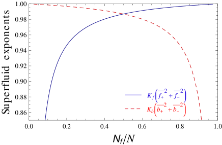
Figure 1: Superfluid exponents for $K_{b}=1$ and $U_{bf}/v_{0}=1$, with $v_{0}=(v_{f}+v_{b})/2$, as a function of the fraction of fermions. We take equal masses for both species, so that $U_{bf}/v_{0}$ is kept a constant for all fillings. Solid blue line: fermions. Red dashed line: bosons.

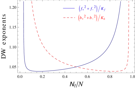
Figure 2: Density wave exponents for $K_{b}=1$ and $U_{bf}/v_{0}=1$, with $v_{0}=(v_{f}+v_{b})/2$, as a function of the fraction of fermions. We take equal masses for both species, so that $U_{bf}/v_{0}$ is kept a constant for all fillings. Solid blue line: fermions. Red dashed line: bosons

In the system under consideration there are three independent parameters, the ratio of velocities $t=v_{f}/v_{b}$, the Luttinger parameter of bosons $K_{b}$ ($K_{f}$ is fixed and equal to 1), and Bose-Fermi interactions, through $U_{bf}$. As an example we plot the superfluid and density wave exponents in Fig. 1 and Fig. 2 respectively, taking $K_{f}=K_{b}=1$, corresponding to hard core bosons and noninteracting fermions. Also we have taken equal masses ($M_{f}=M_{b}=M$) for both species. In that case (and since we are working here in the continuum), $v_{f}=\pi\rho_{f}/M$ and $v_{b}=\pi\rho_{b}/M$ and the ratio of velocities can be expressed as a function of the fraction of fermions only $N_{f}/N$ ($N$ the total number of particles being fixed). For Bose-Fermi interactions, we use the following dimensionless parameter $U_{bf}/v_{0}$ with $v_{0}=(v_{f}+v_{b})/2$ the mean velocity, which is a constant independent of $N_{f}/N$. We wish to illustrate here that the ratio of velocity is a crucial parameter that is ultimately related to clear parameters of an experimental system, such as the number of particles. In Fig. 1 and Fig. 2 one notices that density wave correlations are mostly suppressed for the slowest species of the two, while on the contrary, its superfluid correlations are enhanced. One has to keep this feature in mind which will be crucial for the analysis of localization.

III Localization in 1D Bose-Fermi mixtures

III.1 A preliminary variational argument

Consider the case of a single species of interacting particles with backscattering on a random external potential. We recast ist low-energy Hamiltonian (see (II.1)) into

$$H = \frac{v}{2\pi}\int dx\left[K(\nabla\theta)^{2}+\frac{1}{K}(\nabla\phi)^{2}\right]$$ (40)

$$+ \rho\int dx\left[\xi(x)e^{-i2\phi(x)}+H.c.\right],$$

where again $\xi(x)$ is the $2\pi\rho$ Fourier component of the random potential. We briefly review the variational argument proposed by Fukuyama and Suzumura in Ref. Suzumura and Fukuyama, 1983. It starts by looking for a classical configuration $\phi_{0}(x)$ satisfying

$$\left.\frac{\delta H}{\delta\phi}\right|_{\phi=\phi_{0}}=0,$$ (41)

a differential equation with random coefficients. A variational solution is found by assuming that the charge density wave breaks into domains of size $L_{0}$ on which $\phi_{0}(x)$ is a constant. By doing so it takes advantage from the random potential ($\xi$ and $\xi^{*}$) as much as possible. A typical energy of order $-(L/L_{0})\sqrt{DL_{0}}$ is gained in this way. However, the optimal value $\phi_{0}$ varies randomly from domain to domain with differences of order $\pi$. This costs elastic energy, through the interaction term $(\nabla\phi)^{2}$, of order $L/L_{0}$ if domain walls are of the same typical size $L_{0}$. According to this Imry-Ma-like analysisImry and Ma (1975), there is always a finite value $L_{0}$ for which the energy is minimum and negative (as compared to the value of zero one would obtain for $\phi_{0}$ constant over the whole system). As a next step, quantum fluctuations are added self-consistently. These tend to reduce the amount of potential energy gained from the random potential. Expanding $\phi(x)$ around the classical solution $\phi_{0}(x)$, $\phi(x)=\phi_{0}(x)+\psi(x)$ with $\psi$ a quantum field, the effective Hamiltonian per unit length and up to a constant is:

$$H/L = E_{\text{el}}+\frac{v}{2\pi}\int dx\left[K(\nabla\theta)^{2}+\frac{1}{K}:(\nabla\psi)^{2}:\right]$$ (42)

$$- \left(\frac{D}{L_{0}}\right)^{1/2}\left(\frac{m}{\Lambda}\right)^{K}\int dx:\cos[2\psi(x)]:,$$

where we have normal-ordered the effective sine-Gordon HamiltonianColeman (1975) and $E_{\text{el}}$ is the elastic energy (of order $1/L_{0}$) coming from the classical configuration. $\Lambda$ is a UV cut-off and the mass $m$ can be obtained using a self-consistent harmonic approximationSuzumura and Fukuyama (1983), $m^{2}=\mathcal{B}\sqrt{D/L_{0}}(m/\Lambda)^{K}$, with $\mathcal{B}$ some unimportant prefactor. Minimizing the energy with respect to $L_{0}$ one then finds

$$L_{0}\propto\left(\frac{1}{D}\right)^{\frac{1}{3-2K}},\ \text{for}\ K<3/2.$$ (43)

In the context of 1D interacting particles this length can be understood as the localization length of the system. The CDW is pinned by the random potential and correlations in the phase of the CDW are lost above the localization length. It appears from (43) that $L_{0}$ diverges as $K$ approaches $3/2$. Therefore a gas of 1D fermions should undergo a transition from a localized to superfluid phase as attractive interactions are increased. Similarly for bosons, a transition to superfluidity would occur as interactions are decreased from the hard-core limit. A schematic description of the pinning as understood from the variational solution is given in Fig. 3.

Figure 3: Schematic representation of the phase $\phi(x)$ from the variational solution for the pinning of a density wave by a random potential. The system breaks into domains of order $L_{0}$ separated by domain walls of the same average size. A schematic description of the classical density also appears. $x$ is in unit of the inverse density. On a domain with constant $\phi$ a regulare DW appears while on domain walls, an extra particle ($\nabla\phi<0$) or a hole ($\nabla\phi>0$) is pinned by disorder.

Turning now to the case of an interacting BF mixture, similar arguments can be put forward. Consider the classical solution that minimizes the energy

$$E= \frac{v_{f}}{2\pi K_{f}}\int dx(\nabla\phi_{f})^{2}+\frac{v_{b}}{2\pi K_{b}}\int dx(\nabla\phi_{b})^{2}$$

$$+ \frac{U_{bf}}{\pi^{2}}\int dx\ \nabla\phi_{f}\nabla\phi_{b}$$

$$+ \sum_{\alpha=f,b}\rho_{\alpha}\int dx\left[\xi_{\alpha}(x)e^{-i2\phi_{\alpha}(x)}+H.c.\right].$$ (44)

In the simpler case where the random potential couples only to bosons, the situation is very similar to the one exposed in the single species problem. The boson gas breaks up into domains of size $L_{b}$, on which the classical phase $\phi_{b,0}$ adjusts to the random phase. The fermionic density wave then deforms its phase so as to minimize the energy of the system. There are two elastic contributions for fermions: $(\nabla\phi_{f,0})^{2}$ that tries to keep the fermionic phase constant and $U_{bf}/\pi^{2}\nabla\phi_{f,0}\nabla\phi_{b,0}$ that tries to keep both density waves in phase ($U_{bf}<0$) or out of phase ($U_{bf}>0$). The optimal configuration is readily exhibited by recasting the Hamiltonian in the following form:

$$E= \frac{v_{f}}{2\pi K_{f}}\int dx(\nabla\widetilde{\phi}_{f})^{2}$$

$$+ \frac{v_{b}}{2\pi K_{b}}\left(1-\frac{U_{bf}}{\pi^{2}}\frac{K_{b}K_{f}}{{}^{2}v_{f}v_{b}}\right)\int dx(\nabla\phi_{b})^{2}$$

$$+ \rho_{b}\int dx\left[\xi_{b}(x)e^{-i2\phi_{b}(x)}+H.c.\right],$$ (45)

where we have made the following change of variables, $\widetilde{\phi}_{f}=\phi_{f}+\frac{U_{bf}}{\pi}\frac{K_{f}}{v_{f}}\phi_{b}$. The elastic energy cost of deforming the bosonic phase is reduced by a factor $1-g^{2}$ if $\tilde{\phi}_{f}$ is kept constant. Then, the bosonic gas breaks into domains of size $L_{b}$,

$$L_{b}\propto\left(\frac{1}{D_{b}}\right)^{\frac{1}{3-2\tilde{K}_{b}}},\ \text{for}\ \tilde{K}_{b}<3/2,$$ (46)

with $\tilde{K}_{b}=K_{b}/\sqrt{1-g^{2}}$, while the fermionic density adjusts accordingly in a way given by the classical solution:

$$\phi_{f,0}(x)=-\frac{U_{bf}}{\pi}\frac{K_{f}}{v_{f}}\phi_{b,0}(x)+\text{cste}.$$ (47)

We emphasize two important aspects at this point. Note that the instability toward phase separation or collapse when $g^{2}=1$ is apparent already at the classical level. The coefficient before $(\nabla\phi_{b})^{2}$ becomes negative as $g^{2}$ exceeds $1$, favoring maximum distortion of the bosonic density wave. Note also that the present transformation for the fields (III.1) does not diagonalize the full quantum Hamiltonian, and would not allow for a correct treatment of quantum fluctuations.

Finally, we consider the situation where the disorder couples to both components of the gas. Although a full self-consistent treatment is needed, here we only give a few qualitative arguments; we postpone the self-consistent calculation to section III.3 where we use replica-symmetry breaking in order to describe the fully localized phase. We are now in a situation where the disorder tries to pin both components of the gas independently (as $\xi_{f}$ and $\xi_{b}$ are uncorrelated) while elastic deformations are coupled. We still look for a solution where both components break into domains of size $L_{b}$ and $L_{f}$. A way to disentangle the problem is to consider the case where one of the localization lengths is (much) larger than the other, say $L_{b}>L_{f}$. Building on equation (47), it seems reasonable to assume that the fermionic phase is of the form:

$$\phi_{f,0}(x)=-\frac{U_{bf}}{\pi}\frac{K_{f}}{v_{f}}\phi_{b,0}(x)+\lambda_{f}.$$ (48)

Here, $\lambda_{f}$ which is related to the random phase of the disordered potential $\xi_{f}$ has replaced the constant in equation (47). On domains where $\phi_{b}$ is a constant, $\phi_{f}$ makes random jumps of order $\pi$ to accommodate the random potential, very much as in the single species case. On the contrary, when $\phi_{b}$ deforms between two domains, it has the effect of a chemical potential – much like in a Mott-$\delta$ transition – and imposes a finite slope on $\phi_{f}$. In that case the variations of $\phi_{f}$ follow a nested pattern, in the sense that the coupling to bosons imposes variations on a length scale of the order of $L_{b}$, while each domain of size $L_{b}$ breaks down into smaller domains of size $L_{f}$ in order to accommodate the random phase of the disorder. Of course at this level one should take into account quantum fluctuations. It is the object of the next two sections. First we perform a renormalization group calculation in order to identify the regions of parameter space where disorder is relevant and likely to pin one or both components of the gas. Then we use the concept of replica symmetry breaking to confirm the findings of the RG calculation and the intuitions we got from the classical approach.

III.2 Renormalization Group calculation and a tentative phase diagram

The RG approach is especially powerful to treat both the effects of interactions and disorder in 1D systems. Following the approach introduced by Giamarchi and Schulz in Ref. Giamarchi and Schulz, 1988, we treat disorder as a perturbation of the Luttinger liquid fixed point. Our starting point is the Hamiltonian of equation (II.1). The low-energy fixed point is the two-component Luttinger liquid described in section II.2 and, once again, the random potential tries to pin each component independently. The RG transformation is constructed by integrating out high energy degrees of freedom – here, short distance density fluctuations – at the level of the partition function, through a rescaling of the UV cut-off. A detailed calculation is presented in appendix B. A complication arises in a system with quenched disorder. There, the thermodynamic quantity of interest is the average free energy $F$ defined as:

$$-\beta F=\overline{\log Z}$$ (49)

where $Z$ is the partition function for a given realization of the random potential, and $\overline{\phantom{i}\ldots\phantom{i}}$ denotes averaging over all possible realizations of the disorder. The average free energy is very difficult to compute and one way of action is to use the so-called replica trick Mézard et al. (1987). It rests upon the following observation,

$$\lim\limits_{n\rightarrow 0}\frac{1}{n}\log\overline{Z^{n}}=\overline{\log Z}.$$ (50)

The trick consists in introducing $n$ identical copies of the system, average over the disorder realizations and in the end take the limit $n\rightarrow 0$. Practically we will work with the quantity $\overline{Z^{n}}$ to perform the RG calculation. Using the path integral formulation, the partition function $Z$ for a given realization of the disorder is

$$Z=\int D\phi_{f}D\phi_{b}\ e^{-S[\phi_{f},\phi_{b}]}\;,$$ (51)

with $S$ the action derived from the Hamiltonian (II.1), that is, $S=S_{0}+S_{\text{dis}}$, with:

$$S_{0}=\sum_{\alpha=f,b} \frac{1}{2\pi K_{\alpha}}\int dxd\tau\left[\frac{1}{v_{\alpha}}\left(\partial_{\tau}\phi_{\alpha}\right)^{2}+v_{\alpha}\left(\partial_{x}\phi_{\alpha}\right)^{2}\right]$$

$$+ \frac{U_{bf}}{\pi^{2}}\int dxd\tau\ \partial_{x}\phi_{f}\partial_{x}\phi_{b},$$ (52)

$$S_{\text{dis}}=\sum_{\alpha=f,b} \rho_{\alpha}\int dxd\tau\left[\xi_{\alpha}(x)e^{-2\phi_{\alpha}(x,\tau)}+H.c.\right].$$ (53)

Assuming that $\xi_{f}$ and $\xi_{b}$ have Gaussian distributions, we compute the replicated action defined through:

$$\overline{Z^{n}}=\int\prod_{a=1}^{n}D\phi_{f}^{a}D\phi_{b}^{a}\ e^{-S_{\text{rep}}},$$ (54)

and find $S_{\text{rep}}=S_{0}^{\text{rep}}+S_{\text{dis}}^{\text{rep}}$ with

$$S_{0}^{\text{rep}} =\sum_{a=1}^{n}\sum_{\alpha=f,b}\frac{1}{2\pi K_{\alpha}}\int dxd\tau\left[\frac{1}{v_{\alpha}}\left(\partial_{\tau}\phi^{a}_{\alpha}\right)^{2}+v_{\alpha}\left(\partial_{x}\phi^{a}_{\alpha}\right)^{2}\right]$$ (55)

$$+\frac{U_{bf}}{\pi^{2}}\int dxd\tau\ \partial_{x}\phi^{a}_{f}\partial_{x}\phi^{a}_{b},$$

$$S_{\text{dis}}^{\text{rep}} =-{D_{f}\rho_{f}^{2}}\sum_{a,b}\int dxd\tau d\tau^{\prime}\cos[2\phi_{f}^{a}(x,\tau)-2\phi_{f}^{b}(x,\tau^{\prime})]$$ (56)

$$-{D_{b}\rho_{b}^{2}}\sum_{a,b}\int dxd\tau d\tau^{\prime}\cos[2\phi_{b}^{a}(x,\tau)-2\phi_{b}^{b}(x,\tau^{\prime})]\;.$$

Using the following parametrization for the UV cut-off, $\Lambda(l)=\Lambda_{0}e^{-l}$, $\Lambda_{0}$ being the bare cut-off, we find the following RG flow equations (see Appendix B)

$$\frac{d\tilde{D}_{f}}{dl} = (3-X_{f})\tilde{D}_{f}(l),$$ (57)

$$\frac{d\tilde{D}_{b}}{dl} = (3-X_{b})\tilde{D}_{b}(l),$$ (58)

where we have defined the dimensionless couplings $\tilde{D}_{f}=\frac{D_{f}\rho_{f}^{2}}{v_{f}^{2}\Lambda^{3}}$ and $\tilde{D}_{b}=\frac{D_{b}\rho_{b}^{2}}{v_{b}^{2}\Lambda^{3}}$. $K_{f},K_{b},v_{f}$ and $v_{b}$ are also renormalized. Their flow equations are written in appendix B. The anomalous dimensions, $X_{f}$ and $X_{b}$, of the disorder operators are obtained from the diagonalization of $S_{0}$. They are $X_{f}=2f_{+}^{2}+2f_{-}^{2}$ and $X_{b}=2b_{+}^{2}+2b_{-}^{2}$. We recall their analytical expressions as a function of $t=v_{f}/v_{b}$ and $g$:

$$X_{f} = \frac{2K_{f}}{\sqrt{1-g^{2}}}\frac{1+t\sqrt{1-g^{2}}}{\sqrt{1+2t\sqrt{1-g^{2}}+t^{2}}},$$ (59)

$$X_{b} = \frac{2K_{b}}{\sqrt{1-g^{2}}}\frac{t+\sqrt{1-g^{2}}}{\sqrt{1+2t\sqrt{1-g^{2}}+t^{2}}}.$$ (60)

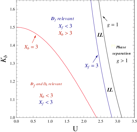
Figure 4: Critical lines as obtained from the RG flow (57) and (58), for a ratio of velocities $t=3$, and $K_{f}=1$. Here we have chosen to parametrize interactions as $U=U_{bf}/\sqrt{v_{f}v_{b}}$.

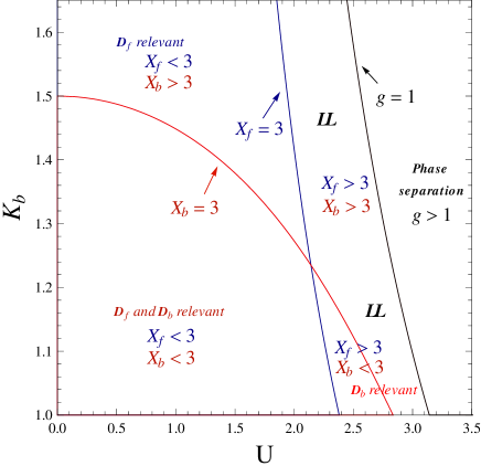
Figure 5: Critical lines as obtained from the RG flow (57) and (58), for a ratio of velocities $t=1/3$, and $K_{f}=1$. We have defined $U=U_{bf}/\sqrt{v_{f}v_{b}}$.

For uncoupled species ($g=0$), $X_{f}=2K_{f}$ and $X_{b}=2K_{b}$. Thus spinless fermions (bosons) are localized when $K_{f}<3/2$ ($K_{b}<3/2$).Giamarchi and Schulz (1988) As Bose-Fermi interactions are turned on, new phases appear. As explained in section II.2, Bose-Fermi interactions tend to enhance superfluid correlations and impair the formation of density waves. Formally, $X_{f}>2K_{f}$ and $X_{b}>2K_{b}$ and there exist regions of parameters for which disorder is an irrelevant perturbation in the RG sense although single species would be localized. In the variational language of section III.1, it means that quantum fluctuations are enhanced by the Bose-Fermi interactions and tend to reduce the localization length.

In Figs. 4 and 5 we show two examples of the critical lines for two ratios of velocities, $v_{f}/v_{b}=3$ and $v_{f}/v_{b}=1/3$. Although the mechanism by which superfluidity is enhanced seems clear enough one should be careful in drawing conclusions about the actual phase diagram from the positions of the critical lines given by Eqs. (57) and (58). Indeed, when one or both perturbations are relevant, disorder parameters flow to a strong coupling phase, out of reach of the perturbative RG we have used so far. This is of special importance in some regions of the phase diagram. For instance in Fig. 4, there is a large portion of the diagram for which $X_{b}>3$ and $X_{f}<3$. Here $D_{f}$ appears to be relevant while $D_{b}$ is irrelevant. If $K_{b}>3/2$ the nature of this phase is quite clear: fermions are localized (they are in the so-called Anderson glass phase) while bosons remain superfluid. Indeed, if $U_{bf}=0$, spinless fermions are localized, as they should be, and bosons are in a superfluid phase ($K_{b}>3/2$). The effects of non-zero BF interactions are two-fold. The phonons of the bosonic gas mediate an effective attractive interactions that eventually leads to a transition to a phase where fermions are superfluid (and pair correlation are dominant). Similarly the phonons of the fermionic gas tend to reduce the repulsion between bosons and enhance superfluidity. Note that although fermions are localized this mechanism is possible since their localization length $L_{f}$ is quite large in the limit of weak disorder and phonons do exist below $L_{f}$. Now if $K_{b}<3/2$ the interpretation of the RG flow is more delicate. Phonons in the fermionic gas do renormalize the bosonic interactions in such a way that $X_{b}>3$ and $D_{b}$ is irrelevant. However as soon as the UV cut-off is rescaled down to the inverse fermionic localization length, fluctuations in the fermionic density are pinned by disorder and ’gapped’, and thus no longer affect the bosons. Below this cut-off, bosons interact with their bare interactions and, as $K_{b}<3/2$, disorder is relevant again and bosons are localized. Therefore above a certain value $l=l_{f}$ for which $\tilde{D}_{f}(l_{f})=1$ and $L_{f}^{-1}=\Lambda(l_{f})$, the flow of $\tilde{D}_{b}$ should be modified as follows:

$$\frac{d\textrm{log}\tilde{D}_{b}}{dl}=\left\{\begin{array}[]{ll}3-X_{b}&\mbox{ if $\Lambda\gg L_{f}^{-1}$}\\ 3-2K_{b}&\mbox{ if $\Lambda\ll L_{f}^{-1}$}.\end{array}\right.$$ (61)

This should hold for any value of $K_{b}$. The important point here is that when $X_{b}>3$ and $K_{b}<3/2$ bosons are still localized once the fermions become localized. However, the structure of the flow indicates that the bosonic localization length (defined as $L_{b}=\Lambda(l_{b})^{-1}$ with $\tilde{D}_{b}(l_{b})=1$) will be extremely large.

Therefore, based on this RG approach we propose the following tentative phase diagram, summarized in Fig. 6 for $v_{f}/v_{b}>1$. We identify three phases: the usual two-component Luttinger liquid (LL) as disorder is irrelevant for both species, a phase where fermions are localized while bosons remain superfluid and a phase where both species are localized but still coupled. We call the latter a Bose-Fermi glass, by analogy with the Bose glass phase. In this phase, despite localization, interactions have very important effects. Notably, the localization length of bosons varies greatly with interactions. We highlight a crossover regime where the boson localization length becomes much larger than the fermion localization length as indicated by (61).

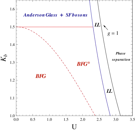
Figure 6: Phase diagram of the Bose-Fermi mixture in a random potential as a function of $K_{b}$ and $U=U_{bf}/\sqrt{v_{b}v_{f}}$ for $t=3$. BFG stands for Bose-Fermi glass. BFG^∗ is the same phase, however we identify a crossover regime for which the localization length of bosons is much larger than the one of fermions.

To confirm our findings we look for a variational solution in replica space. This is the subject of the next section.

III.3 Variational calculation in replica space

III.3.1 Self-consistent equations

In the study of one dimensional systems, a variational calculation if often a complementary tool with respect to, e.g., a renormalization group calculation. We find that, in our case, even if the RG can provide some information on the structure of the phase diagram, it fails to describe properly strong disorder phases. An example was given in the previous subsection, in which once the fermionic disorder has flown to strong coupling – beyond the reach of perturbation theory – the behavior of bosons became unclear, regardless of what we should conclude from the dimension of the disorder operator.

The variational method aims at finding the best Gaussian approximation to the complicated action $S_{\text{rep}}$. It builds on the knowledge that there exists a phase where it is energetically favorable to lock the field $\phi$ to a certain value, and considers only quadratic fluctuations around this minimum value. Within the replica formalism we actually look for a distribution of these optimal values, very much like the solution in Fig. 3. Complications arise, however, since replicas are coupled and one needs to take the limit $n\rightarrow 0$ in the end. We have seen that the RG to first order is replica symmetric. However, to describe the localized phases properly, it is necessary to study solutions which break replica symmetry in the limit $n\rightarrow 0$.

The concepts we will use in this section have been introduced by Parisi and M’ezard in Ref. [Marc Mézard and Giorgio Parisi, 1991] and further developed by Le Doussal and Giamarchi in Ref. [Giamarchi and Le Doussal, 1996] to study the problem of interacting electrons in a disordered potential. Here we generalize the method to the case of two coupled species. Let us fix a few notations before turning to the main points of the calculation, details of which can be found in Appendix C. We rewrite the action $S_{0}$ in Fourier space as

$$S^{0}=\frac{1}{2}\frac{1}{\beta L}\sum_{q,i\omega_{n}}\phi_{\alpha}^{a}(q,i\omega_{n})(G_{0}^{-1})_{\alpha\beta}^{ab}(q,i\omega_{n})\phi_{\beta}^{b}(-q,-i\omega_{n}),$$ (62)

where $\alpha,\beta$=$f,b$ while Latin indices $a,b$ run from 1 to $n$, the number of replicas. There are two implicit summations over $\alpha,\beta$ and $a,b$. $(G_{0}^{-1})_{\alpha\beta}^{ab}$ is a $2n\times 2n$ matrix whose structure is:

$$G_{0}^{-1}=\left(\begin{array}[]{cc}\frac{v_{f}}{\pi K_{f}}\left[\frac{\omega_{n}^{2}}{v_{f}^{2}}+q^{2}\right]{1}_{n}&\frac{U_{bf}}{\pi^{2}}q^{2}{1}_{n}\\ \\ \frac{U_{bf}}{\pi^{2}}q^{2}{1}_{n}&\frac{v_{b}}{\pi K_{b}}\left[\frac{\omega_{n}^{2}}{v_{b}^{2}}+q^{2}\right]{1}_{n}\end{array}\right)$$ (63)

with ${1}_{n}$ the $n\times n$ unit matrix. As stated earlier, we want to replace $S_{rep}$ by its best Gaussian approximation, $S_{G}$, with

$$(G^{-1})_{\alpha\beta}^{ab}=(G_{0}^{-1})_{\alpha\beta}^{ab}-\sigma_{\alpha\beta}^{ab},$$ (64)

and $\sigma_{\alpha\beta}^{ab}$ the self-energy. The best $G$ is obtained by minimizing the variational free energy, $F_{\rm var}$=$F_{G}+\langle S-S_{G}\rangle_{G}/\beta$ with respect to $G_{\alpha\beta}^{ab}$. We find the following expression for $F_{var}$:

$$F_{var} = -\frac{1}{2\beta}\sum_{q,i\omega_{n}}\textrm{Tr}\log[G(q,i\omega_{n})]$$ (65)

$$+ \frac{1}{2}\sum_{\alpha,\beta}\sum_{q,i\omega_{n}}\left(G_{0}^{-1}\right)_{\alpha\beta}(q,i\omega_{n})\textrm{Tr}[G_{\alpha\beta}(q,i\omega_{n})]$$

$$+ \frac{1}{2}\sum_{a,b}L\int d\tau\left[V_{F}[F^{ab}(\tau)]+V_{B}[B^{ab}(\tau)]\right]$$

with:

$$F^{ab}(\tau) = \langle\left[\phi_{f}^{a}(x,\tau)-\phi_{f}^{b}(x,0)\right]^{2}\rangle_{G},$$ (66)

$$B^{ab}(\tau) = \langle\left[\phi_{b}^{a}(x,\tau)-\phi_{b}^{b}(x,0)\right]^{2}\rangle_{G},$$ (67)

and $V_{F}(x)=-2{\rho_{f}^{2}D_{f}}e^{-2x}$ and $V_{B}(x)=-2{\rho_{b}^{2}D_{b}}e^{-2x}$. In the case of static disorder, off-diagonal quantities (say, $F^{ab}$ or $B^{ab}$ with $a\neq b$) do not depend on timeGiamarchi and Le Doussal (1996). This is because off-diagonal elements describe correlations between replicas locked to different minima, but experiencing the same disorder. The experienced random potential being static, these correlations are also time-independent. Bearing this in mind we then derive the following saddle-point equations:

$$\sigma_{ff}^{aa}(q,\omega_{n}) = 2\int_{0}^{\beta}d\tau\left(1-\cos[\omega_{n}\tau]\right)V^{\prime}_{F}(F^{aa}(\tau))$$ (68)

$$+ 2\int_{0}^{\beta}d\tau\sum_{b\neq a}V_{F}^{\prime}[F^{ab}],$$

$$\sigma_{bb}^{aa}(q,\omega_{n}) = 2\int_{0}^{\beta}d\tau\left(1-\cos[\omega_{n}\tau]\right)V^{\prime}_{B}(B^{aa}(\tau))$$ (69)

$$+ 2\int_{0}^{\beta}d\tau\sum_{b\neq a}V_{B}^{\prime}[B^{ab}],$$

$$\sigma_{ff}^{ab}(q,\omega_{n}) = -2\beta\delta_{n,0}V^{\prime}_{F}(F^{ab})\;\;\;(a\neq b),$$ (70)

$$\sigma_{bb}^{ab}(q,\omega_{n}) = -2\beta\delta_{n,0}V^{\prime}_{B}(B^{ab})\;\;\;(a\neq b),$$ (71)

$$\sigma_{fb}^{ab}(q,\omega_{n}) = \sigma_{bf}^{ab}(q,\omega_{n})=0\;\;\;\;\;\;\;(\forall\ a,b).$$ (72)

The next step is to take the limit $n\rightarrow 0$. We follow Parisi’s parameterization of $0\times 0$ matrices.Marc Mézard and Giorgio Parisi (1991) If $A$ is a matrix in replica space, taking $n$ to $0$, it can be parameterized by a couple $(\tilde{a},a(u))$, with $\tilde{a}$ corresponding to the (equal) replica-diagonal elements and $a(u)$ a function of $u\in[0,1]$, parameterizing the off-diagonal elements. Then the self-energy matrix is expressed as

$$\sigma(q,\omega_{n}=0)=\left(\begin{array}[]{cc}[\tilde{\sigma}_{f},\sigma_{f}(u)]&0\\ \\ 0&[\tilde{\sigma}_{b},\sigma_{b}(u)]\end{array}\right)\;.$$ (73)

Then we proceed to invert $G^{-1}$ in order to solve the saddle-point equations. To do so we are led to make assumptions on the off-diagonal functions $\sigma_{f}(u)$ and $\sigma_{b}(u)$. Either we look for replica-symmetric (RS) solutions, with constant $\sigma_{f}(u)$ and/or $\sigma_{b}(u)$, or replica symmetry breaking (RSB) solutions, with non-constant off-diagonal functions. First shall we focus on the phase with localized fermions and superfluid bosons then on the phase in which both species are pinned. In both cases we find a consistent solution by first making an intelligent guess for the structure of the replica symmetry-breaking solution, and then verifying its stability.

III.3.2 Phase with localized fermions and superfluid bosons

As was shown in Ref. [Giamarchi and Le Doussal, 1996], the localized phase of fermions in a disordered potential is well-described by a RSB solution. More precisely, a level 1 symmetry breaking is required to describe the localized phase. It means that $\sigma_{f}(u)$ is a step function, $\sigma_{f}(u<u_{f})=0$ and $\sigma_{f}(u>u_{f})=1$, with $u_{f}$ a breaking point that needs to be fixed. To describe the phase with localized fermions and free bosons that is predicted by the RG, we look for a solution with level 1 RSB in the fermionic sector and replica symmetry in the bosonic sector. The details of the calculation are presented in Appendix C.

We introduce the inverse connected Green functionGiamarchi and Le Doussal (1996),

$$(G^{-1})^{c}_{\alpha\beta}\equiv\lim_{n\rightarrow 0}\sum\limits_{b}(G^{-1})^{ab}_{\alpha\beta},$$ (74)

which, using Parisi’s notation becomes

$$(G^{-1})^{c}_{\alpha\beta}=\widetilde{G^{-1}}_{\alpha\beta}-\int_{0}^{1}du\ G^{-1}_{\alpha\beta}(u)\;.$$ (75)

For this choice of replica symmetry breaking it can be cast into

$$(G^{-1})^{c}_{ff} = (G_{0}^{-1})_{ff}(q,i\omega_{n})+I_{F}(\omega_{n})+\Sigma_{F}(1-\delta_{n,0}),$$

$$(G^{-1})^{c}_{bb} = (G_{0}^{-1})_{bb}(q,i\omega_{n})+I_{B}(\omega_{n}),$$

$$(G^{-1})^{c}_{fb} = (G^{-1})^{c}_{bf}=(G_{0}^{-1})_{fb}(q,i\omega_{n}),$$ (76)

where

$$I_{f}(\omega_{n}) = 2\int_{0}^{\beta}d\tau\left(1-\cos[\omega_{n}\tau]\right)\times(V^{\prime}_{F}[\widetilde{F}(\tau)]-V_{F}^{\prime}[F]),$$

$$I_{b}(\omega_{n}) = 2\int_{0}^{\beta}d\tau\left(1-\cos[\omega_{n}\tau]\right)V^{\prime}_{B}[\widetilde{B}(\tau)],$$

and

$$\Sigma_{F}=2\beta u_{f}V^{\prime}_{F}[F].$$ (79)

The structure of the connected propagator allows to identify several features of the RSB solutions. A mass term $\Sigma_{F}$ is here generated and we will confirm later in this section that it indeed controls the localization length. However $(G^{-1})^{c}_{ff}(q=0,\omega_{n}=0)$ is still $0$, as it should for a system that is, after averaging on disorder, translationaly invariant. Finally, RSB endows the Green’s functions with a new dynamical content through the functions $I_{F}(\omega_{n})$ and $I_{F}(\omega_{n})$.

The system of equations is effectively closed by writing an equation for the breaking point $u_{f}$. This is done, by inspecting the stability of such a solution and explicitely requiring the marginality of the so-called replicon mode. This choice is made on physical grounds – as it gives sensible results for dynamical quantities, such as the conductivity – following the path set in Ref. Giamarchi and Le Doussal, 1996 (details about the calculation are given in appendix C). Finally, equation (79) is replaced by

$$\Sigma_{f}^{3/2}=\frac{8}{\sqrt{1-g^{2}}}{\rho_{f}^{2}D_{f}}\left(\frac{\pi K_{f}}{v_{f}}\right)^{1/2}e^{-2F}$$ (80)

Note that $F$, $\widetilde{F}$ and $\widetilde{B}$ are obtained through inversion of $G^{-1}$. They read

$$F=\frac{2}{\beta L}\sum_{q,i\omega_{n}}\frac{\pi K_{f}}{v_{f}}\frac{\left(\frac{\omega_{n}^{2}}{v_{b}^{2}}+q^{2}+\hat{I}_{b}(\omega_{n})\right)}{\left(\frac{\omega_{n}^{2}}{v_{b}^{2}}+q^{2}+\hat{I}_{b}(\omega_{n})\right)\left(\frac{\omega_{n}^{2}}{v_{f}^{2}}+q^{2}+\hat{I}_{f}(\omega_{n})+\hat{\Sigma}_{f}\right)-g^{2}q^{4}}$$ (81)

$$\widetilde{F}(\tau)=\frac{2}{\beta L}\sum_{q,i\omega_{n}}\frac{\pi K_{f}}{v_{f}}\left(1-\cos[\omega_{n}\tau]\right)\frac{\frac{\omega_{n}^{2}}{v_{b}^{2}}+q^{2}+\hat{I}_{b}(\omega_{n})}{\left(\frac{\omega_{n}^{2}}{v_{b}^{2}}+q^{2}+\hat{I}_{b}(\omega_{n})\right)\left(\frac{\omega_{n}^{2}}{v_{f}^{2}}+q^{2}+\hat{I}_{f}(\omega_{n})+\hat{\Sigma}_{f}\right)-g^{2}q^{4}}$$ (82)

$$\widetilde{B}(\tau)=\frac{2}{\beta L}\sum_{q,i\omega_{n}}\frac{\pi K_{b}}{v_{b}}\left(1-\cos[\omega_{n}\tau]\right)\frac{\frac{\omega_{n}^{2}}{v_{f}^{2}}+q^{2}+\hat{I}_{f}(\omega_{n})+\hat{\Sigma}_{f}}{\left(\frac{\omega_{n}^{2}}{v_{b}^{2}}+q^{2}+\hat{I}_{b}(\omega_{n})\right)\left(\frac{\omega_{n}^{2}}{v_{f}^{2}}+q^{2}+\hat{I}_{f}(\omega_{n})+\hat{\Sigma}_{f}\right)-g^{2}q^{4}}$$ (83)

One can recognize in $F$ and $\widetilde{F}$ the fermionic propagator and in $\widetilde{B}$ the bosonic propagator. We have introduced $\hat{I}_{f}=\frac{\pi K_{f}}{v_{f}}I_{F}$, $\hat{\Sigma}_{F}=\frac{\pi K_{f}}{v_{f}}\Sigma_{F}$, and used similar notations for bosons. The complete numerical solution of this self-consistent set of functional equations is beyond the scope of the present paper, and the presence of the functions $\hat{I}_{f}(\omega_{n})$ and $\hat{I}_{b}(\omega_{n})$ indeed makes the situation complicated. We proceed in several steps in order to analyze the equations.

First we take $\hat{I}_{f}(\omega_{n})$ and $\hat{I}_{b}(\omega_{n})$ to be zero. In this case, our variational approach is analogous to the theory of Fukuyama and Suzumura, summarized in Sec. III.1, however with a more accurate treatment of quantum fluctuations that does not require a detailed knowledge of the underlying classical solution. We show that within this approximation we obtain sensible results in good agreement with the RG results.

First let us refine the RG analysis of Sec. III.2 by looking at the flow of $\tilde{D}_{b}$ when bosons are coupled to localized fermions. To do so, we perturb the Gaussian action $S_{G}$ with a disorder term coupling only to bosons:

$$S=S_{G}-\frac{D_{b}\rho_{b}^{2}}{\Lambda^{3}}\sum_{a,b}\Lambda^{3}\int dxd\tau d\tau^{\prime}\cos[2\phi_{b}^{a}(x,\tau)-2\phi_{b}^{b}(x,\tau^{\prime})]\;.$$ (84)

The quadratic propagator $G$ is replica symmetric in the bosonic sector and has level-1 RSB in the fermionic sector. To obtain the flow of $\tilde{D}_{b}$, we proceed as explained in Appendix B, and integrate out high-momentum degrees of freedom, between $\Lambda^{\prime}$ and the original cut-off $\Lambda$. To first order in $D_{b}$, the flow equation is obtained by requiring that:

$$\tilde{D}_{b}(\Lambda^{\prime})=\tilde{D}_{b}(\Lambda)\left(\frac{\Lambda^{\prime}}{\Lambda}\right)^{-3}\langle e^{i2\phi_{b}^{a}(x,\tau)}\rangle_{>}^{2}.$$ (85)

$\langle e^{i2\phi_{b}^{a}(x,\tau)}\rangle_{>}^{2}$ is only related to the diagonal part of $G_{bb}$, that is $\widetilde{G}_{bb}(q,\omega_{n})$. We find:

$$\langle e^{i2\phi_{b}^{a}(x,\tau)}\rangle_{>}^{2}=\exp\left[-\int_{\Lambda^{\prime}}^{\Lambda}dq\ \mathcal{J}_{b}(q)\right],$$ (86)

with

$$\mathcal{J}_{b}(q)=\frac{2K_{b}\left[t(q^{2}+\hat{\Sigma}_{f})+q\sqrt{q^{2}(1-g^{2})+\hat{\Sigma}_{f}}\right]}{q\sqrt{q^{2}(1-g^{2})+\hat{\Sigma}_{f}}\sqrt{q^{2}(1+t^{2})+t^{2}\hat{\Sigma}_{f}+2tq\sqrt{q^{2}(1-g^{2})+\hat{\Sigma}_{f}}}}.$$ (87)

Finally, by taking $\Lambda^{\prime}=\Lambda(1+dl)$,the flow equation reads

$$\frac{d\log D_{b}}{dl}=3-\Lambda(l)\mathcal{J}_{b}(\Lambda(l)).$$ (88)

$\mathcal{J}_{b}(q)$ has a power law decay at small and large $\Lambda$ but with different prefactors. Indeed:

$$\Lambda\mathcal{J}_{b}(\Lambda) =2K_{b}~{} \textrm{when}~{}\Lambda\ll\left(\hat{\Sigma}_{f}/\sqrt{1-g^{2}}\right)^{1/2},$$ (89)

$$\Lambda\mathcal{J}_{b}(\Lambda) =X_{b}~{} \textrm{when}~{}\Lambda\gg\left(\hat{\Sigma}_{f}/\sqrt{1-g^{2}}\right)^{1/2}.$$ (90)

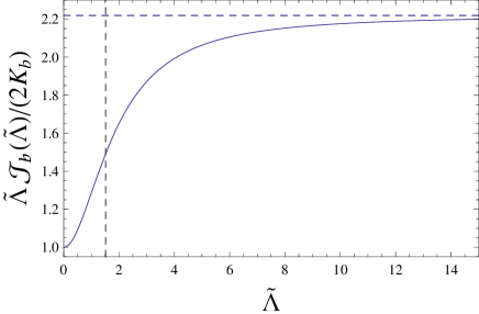
Figure 7: Crossover behavior of the function $\mathcal{J}_{b}$ as defined in Eq. (87), for $t=3$ and $g=0.9$. Here we have plotted $\tilde{\Lambda}\mathcal{J}_{b}(\tilde{\Lambda})/(2K_{b})$, with $\tilde{\Lambda}=\Lambda/\sqrt{\hat{\Sigma}_{f}}$. It goes to $1$ at low momenta and saturates at $X_{b}/(2K_{b})$ as momentum is increased. We identify a crossover region around $\Lambda=(\hat{\Sigma}_{f}/\sqrt{1-g^{2}})^{1/2}$ (vertical dashed line).

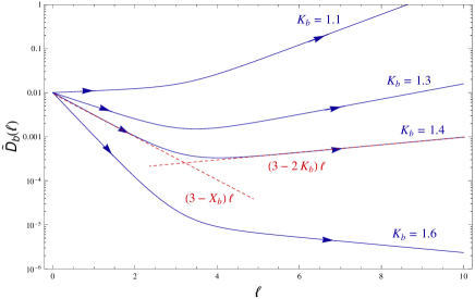
Figure 8: Modified RG flow for bosons using the Gaussian variational solution.

The cross-over of the anomalous dimension appearing in Eq. (88) and the corresponding flow of the disorder are illustrated in Figs. 7 and 8. The flows in Fig. 8 confirm entirely our intuitive arguments in Section III.2. The fermionic mass $\hat{\Sigma}_{f}$ sets a length scale below which bosons interact with their bare interactions. The corresponding length scale can thus be identified as the fermionic localization length, $L_{f}$,

$$L_{f}\equiv\left(\frac{\sqrt{1-g^{2}}}{\hat{\Sigma}_{f}}\right)^{1/2}\;.$$ (91)

We shall return to this equation in the next section when we compute correlation functions for fermions. This RG analysis also confirms that below $K_{b}=3/2$ bosonic disorder is relevant, and the variational solution with RSB only in the fermionic sector is insufficient. To proceed and describe the phase where disorder is relevant for both species we shall need a variational solution with replica symmetry breaking in both the fermionic and the bosonic sector.

III.3.3 Phase with both species pinned by disorder, and complete phase diagram

Case of Faster fermions, $v_{f}>v_{b}$. In this case we found that in the regime with both species localized it is impossible to obtain a self-consistent solution with only level 1 RSB in both sectors, and one needs to allow for level 2 RSB in at least one of the sectors. It turns out, that with level 2 RSB the marginal stability (marginalitly) of the saddle point solution can be satisfied, and that physically meaningful results are thus obtained. Level 2 RSB is thus suffucient to describe this phase. The structure of the solution, and the derivation of the corresponding integral equations are detailed in Appendix C. The resulting (rather complicated) integral equations were solved numerically.

For $v_{f}>v_{b}$ we always find a stable numerical solution with 2RSB for fermions and 1RSB for bosons with the following self-energy structure: $\sigma_{f}(u)$ is a 2-step function, $\sigma_{f}(u<u_{1})=0$, $\sigma_{f}(u_{1}<u<u_{2})=\sigma_{f}^{(1)}$ and $\sigma_{f}(u_{2}<u<1)=\sigma_{f}^{(2)}$, while $\sigma_{b}(u)$ is a 1-step function, $\sigma_{b}(u<u_{2})=0$, $\sigma_{f}(u_{2}<u<u_{1})=\sigma_{b}^{(2)}$. Note that the structure of the solution is reminiscent of the physical arguments we developed in section III.1 for the classical solution. We argued there that in the situation where $L_{b}>L_{f}$ – which is the case in the phase diagram of Fig. 9, and apparent on Figs. 10 and 11 – the fermion density wave should have a nested structure as it breaks into domains to accommodate the random phase and the bosonic density.

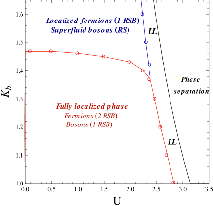
Figure 9: Phase diagram obtained by the Gaussian variational method in replica space as a function of $K_{b}$ and $U=U_{bf}/\sqrt{v_{b}v_{f}}$. We took $\tilde{D}_{f}=\tilde{D}_{b}=0.005$ and $t=v_{f}/v_{b}=3$.

In Figs. 10 and 11 we show examples of the solution for various values of $K_{b}$ as $U_{bf}$ is increased. Note that the fermion mass is related to the 2-step self-energy as

$$\Sigma_{f}=\Sigma_{f}^{(1)}+\Delta\Sigma_{f}^{(2)},$$ (92)

with $\Sigma_{f}^{(1)}=u_{1}\sigma_{f}^{(1)}$, and $\Delta\Sigma_{f}^{(2)}=u_{2}\left(\sigma_{f}^{(2)}-\sigma_{f}^{(1)}\right)$. For the bosonic mass we have $\Sigma_{b}=u_{2}\sigma_{b}^{(2)}$ and $L_{b}=\hat{\Sigma}_{b}^{-1/2}$. The boundary of the region where the level-2 RSB solution exists is obtained by the condition, $\Delta\Sigma_{f}^{(2)}=0$. This condition is fulfilled either when $\Sigma_{f}^{(1)}\neq 0$, $\Sigma_{b}=0$ and the system is in the region with 1 level RSB in the fermionic sector only, or when $\Sigma_{f}^{(1)}=0$, $\Sigma_{b}=0$ and the system is in the replica symmetric phase.

Let us notice two important points here. For any $U_{bf}\neq 0$ we obtain $\hat{\Sigma_{b}}\leq\hat{\Sigma_{f}}$, impying that the fermionic localization length is smaller than the bosonic localization length. There are two reasons for that. First, if $K_{b}>1$, quantum fluctuations are more important for bosons than for fermions (for which $K_{f}=1$), and tend to increase the localization length of bosons with respect to that of fermions (disorder pins the fermion density wave more efficiently). Second, Bose-Fermi interactions enhance superfluid correlations of both components of the mixture. Nevertheless, as we pointed out in Sec. II, superfluid correlations of the slower species are more strongly enhanced. This behavior appears in Figs. 10 and 11, where one can see that the mass of the slow species (here bosons) decreases to extremely small values, long before the true transition to the Luttinger liquid phase takes place, whereas the mass of the fast species (here fermions) is weakly renormalized, excepting the close proximity of the transition. This is a crucial point for the possible observation of the fully localized phase: in a finite-size system, bosons could appear as superfluid simply because their localization length exceeds the size of the trap, even though they should be localized in the thermodynamic limit.

Case of faster bosons, $v_{f}<v_{b}$ Now let us turn to the more delicate case of $v_{b}>v_{f}$. In the RG-based tentative phase diagram of Fig. 5 two intermediate regions appear, where only one of the species appears to be localized. However, for the same reasons as in the previous case $v_{f}>v_{b}$, these two phases are just artifacts of the RG procedure, and in each of them we need to repeat our two step localization argument. Correspondingly, a 2-step RSB shall appear in the variational solution, too. However, before discussing the phase diagram of Fig. 12, let us make a few remarks to gain a reasonable intuition for the results.

In the $v_{b}<v_{f}$ case we had established that the bosonic localization length was always larger than the fermionic one, because of (i) larger quantum fluctuations ($K_{b}\geq K_{f}$) and (ii) because of the enhancement of superluid correlations of the slow species because of interactions. In the present case the situation is somewhat different. Along the line $K_{b}=K_{f}=1$, bosons are now the faster species, and their localization length is now smaller than that of fermions. This translates into an inversion of the levels of symmetry breaking in the fermionic and bosonic sectors. However as soon as $K_{b}>1$, larger quantum fluctuations for bosons counteract this effect, and if $K_{b}$ is large enough, then the bosonic localization length exceeds the fermionic one again, and the order of replica symmetry breaking is reversed .

This can be clearly seen in Fig. 12, where we show the phase diagram emerging from a full numerical solution of the integral equations. We indeed find an inversion of the levels of symmetry breaking. We have to point out here that the numerical solution has a hysteresis: we obtain a different phase boundary by increasing $K_{b}$ at fixed $U_{bf}$ instead of decreasing it. This can be explained by the asymmetric structure of the equations for the 2RSB+1RSB solutions (see Appendix C, $K_{b}$ playing a singular role). The appearing hysteresis could be a signature of a first order transition, too, however, on physical grounds we tend to believe that there is simply a cross-over between the 2RSB+1RSB and 1RSB+2RSB regimes. We emphasize again that the difference between the two cases, $v_{f}>v_{b}$ and $v_{b}>v_{f}$, is related to the inversion of length scales that can only take place for $v_{b}>v_{f}$.

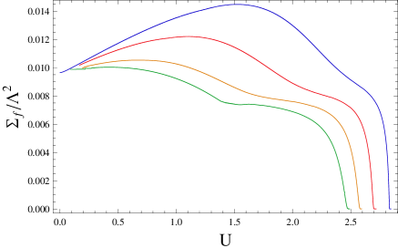
Figure 10: Fermion mass $\hat{\Sigma}_{f}$ and $\Delta\hat{\Sigma}_{f}^{(2)}$ as a function of $U=U_{bf}/\sqrt{v_{f}v_{b}}$, for $t=v_{f}/v_{b}$ and $K_{b}=1,1.1,1.2,1.3$ (top to bottom). Note that $\Delta\hat{\Sigma}_{f}^{(2)}$ goes to zero simultaneously with $\hat{\Sigma}_{f}$ as $U$ is increased.

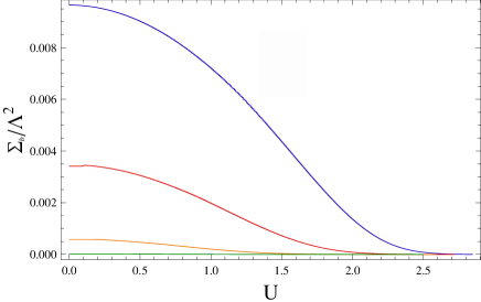
Figure 11: The boson mass $\hat{\Sigma}_{b}$ as a function of $U=U_{bf}/\sqrt{v_{f}v_{b}}$, for $t=v_{f}/v_{b}$ and $K_{b}=1,1.1,1.2,1.3$ (top to bottom). Note that $\hat{\Sigma}_{b}$ goes to zero, simultaneously with $\hat{\Sigma}_{f}$

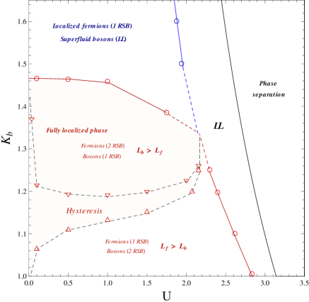
Figure 12: Phase diagram obtained by the Gaussian variational method in replica space for $\tilde{D}_{f}=\tilde{D}_{b}=0.005$ and $v_{f}/v_{b}=1/3$. In the fully localized phase there is crossover between two regions where the order of replica symmetry breaking is reverted.

IV Experimental consequences

In this section we present a few observables that we believe would help to characterize the various phases in an experiment on cold atoms. One possibility is provided by time-of-flight (TOF) experiments, measuring the momentum distribution of the gas inside the trap. For bosons, TOF provides an indirect measurement of the superfluid correlations (and the single-particle Green’s function), the behavior of which varies significantly from the localized to the superfluid phase. Another usual probe is Bragg scattering, giving access to structure factors, that is the Fourier Transform of the density-density correlation functions. The latter quantity we already computed in Ref. Crépin et al., 2010. Here we briefly present how one can compute both density correlations (to compute the structure factor for instance) and superfluid correlations from the variational method. Then we apply these results to study the relevant physical quantities.

IV.1 Density correlations

Density correlations are of the form $\overline{\langle\rho(x,t)\rho(0,0)\rangle}$, where, as usual, brackets stand for the quantum averaging and overlining denotes averaging over disorder realizations. In practice we will use the variational solution in replica space, and more precisely the diagonal Green’s functions. As experimentalists can address each species separately, we will focus on $\overline{\langle\rho_{f}(x,t)\rho_{f}(0,0)\rangle}$ and $\overline{\langle\rho_{b}(x,t)\rho_{b}(0,0)\rangle}$ and shall not consider cross-terms for now. It is instructive to look at the two particular terms

$$C_{f}(x) = \overline{\langle e^{i2\phi_{f}(x)}e^{-i2\phi_{f}(0)}\rangle},$$ (93)

$$C_{b}(x) = \overline{\langle e^{i2\phi_{b}(x)}e^{-i2\phi_{b}(0)}\rangle},$$ (94)

which characterize the $q\approx 2\pi\rho_{b/f}$-momentum density-density correlations (see Eq. 7). In order ot compute $C_{f}$ and $C_{B}$, one first needs to recall the gauge transformation that we performed to get rid of the forward scattering processes. Once included they lead to an exponential decay of $C_{f}$ and $C_{b}$ in every phase, localized or not. The general form of $C_{\alpha}(x)$ is therefore

$$C_{f}(x) = \exp\left[-x/L_{f,{\rm FW}}\right]\times$$ (95)

$$\times \exp\left[-2\frac{1}{\beta L}\sum_{q,\omega_{n}}(1-\cos[qx])\widetilde{G_{ff}}(q,\omega_{n})\right]$$

$$C_{b}(x) = \exp\left[-x/L_{b,{\rm FW}}\right]\times$$ (96)

$$\times \exp\left[-2\frac{1}{\beta L}\sum_{q,\omega_{n}}(1-\cos[qx])\widetilde{G_{bb}}(q,\omega_{n})\right]$$

where

$$L_{f,{\rm FW}} = \frac{(1-g^{2})^{2}}{K_{f}^{2}/v_{f}^{2}}\left[\alpha_{f}-\alpha_{b}g\sqrt{\frac{v_{f}}{v_{b}}\frac{K_{b}}{K_{f}}}\right]^{-2}D_{f}^{-1},$$ (97)

$$L_{b,{\rm FW}} = \frac{(1-g^{2})^{2}}{K_{b}^{2}/v_{b}^{2}}\left[\alpha_{b}-\alpha_{f}g\sqrt{\frac{v_{b}}{v_{f}}\frac{K_{f}}{K_{b}}}\right]^{-2}D_{b}^{-1},$$ (98)

are length scales related to disorder forward scattering. In the localized phases, backscattering also leads to an exponential decay of these correlations functions, and it might therefore be difficult to disentangle contributions from forward and backward scattering. Therefore, experimentally, one should rather focus on correlation functions, which are not influenced by the forward scattering contribution (see Sec. IV.2 and IV.3). It is nevertheless instructive to write down the explicit form of $C_{f}(x)$ and $C_{b}(x)$.

Let us start with the Luttinger liquid phase. There, the mixture is not pinned by disorder and the self-energies $\sigma_{f}$ and $\sigma_{b}$ are zero. The inversion of $G^{-1}$ leads to

$$\widetilde{G_{ff}}(q,\omega_{n}) = \frac{\pi K_{f}}{v_{f}}\frac{q^{2}+b(\omega_{n})}{[q^{2}+b(\omega_{n})][q^{2}+f(\omega_{n})]-g^{2}q^{4}},$$

$$\widetilde{G_{bb}}(q,\omega_{n}) = \frac{\pi K_{b}}{v_{b}}\frac{q^{2}+b(\omega_{n})}{[q^{2}+f(\omega_{n})][q^{2}+f(\omega_{n})]-g^{2}q^{4}}.$$

Here we have introduced the following general notation

$$b(\omega_{n}) = \omega_{n}^{2}/v_{b}^{2}+\hat{I}_{b}(\omega_{n})+\hat{\Sigma}_{b}\;,$$ (101)

$$f(\omega_{n}) = \omega_{n}^{2}/v_{f}^{2}+\hat{I}_{f}(\omega_{n})+\hat{\Sigma}_{f}\;.$$ (102)

In the present case $\hat{\Sigma}_{f}=\hat{\Sigma}_{b}=0$, and therefore we recover the propagators of the Luttinger liquid, with simply a renormalization of the frequency behavior by the functions $\hat{I}_{b}(\omega_{n})$ and $\hat{I}_{f}(\omega_{n})$. Note that these functions are directly proportional to $\tilde{D}_{f}$ et $\tilde{D}_{b}$. Although we have not solved the self-consistency equations for $\hat{I}_{f}(\omega_{n})$ and $\hat{I}_{b}(\omega_{n})$, we expect that in the weak disorder limit they do not modify drastically the propagators. In the Luttinger liquid phase, $C_{f}$ and $C_{b}$ thus decay algebraically at short distances, however, this algebraic decay is cut at long distances by the exponential decay due to disorder-induced forward scattering processes.

Now let us turn to the phase where fermions are localized and bosons superfluid. Here we found a variational solution with 1RSB in the fermionic sector. The inversion of $G^{-1}$ now leads to

$$\widetilde{G_{ff}}(q,\omega_{n}) = \frac{\pi K_{f}}{v_{f}}\Biggl{(}\frac{q^{2}+b(\omega_{n})}{[q^{2}+b(\omega_{n})][q^{2}+f(\omega_{n})]-g^{2}q^{4}}$$ (103)

$$+ \delta_{n,0}\frac{1}{1-g^{2}}\frac{\sigma_{f}}{q^{2}[q^{2}(1-g^{2})+\hat{\Sigma}_{f}]}\Biggr{)}\;,$$

$$\widetilde{G_{bb}}(q,\omega_{n}) = \frac{\pi K_{b}}{v_{b}}\Biggl{(}\frac{q^{2}+f(\omega_{n})}{[q^{2}+b(\omega_{n})][q^{2}+f(\omega_{n})]-g^{2}q^{4}}$$ (104)

$$+ \delta_{n,0}\frac{g^{2}}{1-g^{2}}\frac{\sigma_{f}}{q^{2}[q^{2}(1-g^{2})+\hat{\Sigma}_{f}]}\Biggr{)}\;.$$

In each propagator, the first term controls the algebraic short distance decay of correlations. The second term, once the sum over momenta is done, leads to a long distance exponential decay. Indeed,

$$\frac{1}{L}\sum_{q}\frac{1-\cos[qx]}{q^{2}[q^{2}(1-g^{2})+\hat{\Sigma}_{f}]} =$$ (105)

$$\frac{1}{2\hat{\Sigma}_{f}}\left[x+\sqrt{\frac{1-g^{2}}{\hat{\Sigma}_{f}}}\left(e^{-x\sqrt{\frac{\hat{\Sigma}_{f}}{1-g^{2}}}}-1\right)\right].$$

Furthermore $\sigma_{f}=\beta\frac{v_{f}}{\pi K_{f}}\sqrt{1-g^{2}}\Sigma_{f}^{3/2}$, and one can isolate in $C_{f}$, a decaying exponential of the form

$$C_{f}(x)\sim e^{-x/L_{f}},$$ (106)

with

$$L_{f}=\left(\frac{1-g^{2}}{\hat{\Sigma}_{f}}\right)^{1/2},$$ (107)

which we are tempted to identify with the localization length. Remarkably, although only the fermions are localized, bosonic correlations also display an extra exponential decay, with an exponent smaller by a factor $g^{2}$. This contribution comes directly from the Bose-Fermi interaction term $\nabla\phi_{f}\nabla\phi_{b}$ where $\nabla\phi_{f}$ acts as a random potential inducing forward scattering. The expressions for the propagators in the fully localized phase are given in appendix D. At this stage we think that probing the dynamics of the system, through the dynamical structure factor, would be a better way to test the level of replica symmetry breaking.

IV.2 Structure factors

The dynamical structure factors $S_{b/f}(q,\omega)$ are response functions which can be probed through Bragg scattering experiments.Fallani et al. (2007b); Fabbri et al. (2011) They are defined by

$$S_{b/f}(q,\omega)=\int\int\,{\rm d}t\,{\rm d}x\,e^{iqx-i\omega t}\;\overline{\langle\rho_{b/f}(x,t)\rho_{b/f}(0,0)\rangle}.$$ (108)

Using Eq. (7), we can see that several Fourier components contribute to the structure factors. However, at small momenta, $q\ll 2\pi\rho_{b/f}$, it is essentially given by

$$S_{b/f}(q,\omega)\approx\int\int\frac{{\rm d}t\,{\rm d}x}{\pi^{2}}e^{iqx-i\omega t}\overline{\langle\partial_{x}\phi_{b/f}(x,t)\partial_{x}\phi_{b/f}(0,0)\rangle}$$ (109)

which, in turn, can be computed with the variationnal solution. Note that we ignore here the static contribution from the forward scattering on disorder.Crépin et al. (2010) For fermions it reads:

$$S_{f}({q},\omega)=-\textrm{Im}\left[q^{2}\widetilde{G}_{ff}(q,i\omega_{n}\to\omega+i\epsilon)\right],$$ (110)

and we have a similar expression for bosons. Here, $\widetilde{G}_{ff}$ is the replica-diagonal contribution for the fermion propagator. The complete analytical expression of $S_{f}$ is given in appendix D. To perform the analytical continuation it is necessary to elaborate on the expression of functions $I_{f}$ et $I_{b}$. The only thing that seems analytically feasible is to adapt the argument of Ref. Giamarchi and Le Doussal, 1996 to the case of a mixture. In the fully localized phase, $I_{b}$ and $I_{f}$ are given by equations 162 and 163 of appendix C and one can obtain two simple self-consistent equations by assuming that $K_{f}\ll 1$ and $K_{b}\ll 1$ (thus taking a sort of classical limit) and expanding the functions $V_{f}$ and $V_{b}$ to leading order. In addition, by taking the limit $\Sigma_{b}\ll\Sigma_{f}$ we arrive to the following approximate expressions, at low frequency, $I_{f}(\omega)\sim\alpha_{f}\omega$ and $I_{b}(\omega)\sim\alpha_{b}\omega$ with

$$\alpha_{f} = \sqrt{\Sigma_{f}}\frac{2}{\sqrt{3}}(1+t^{2}g^{2}),$$ (111)

$$\alpha_{b} = \sqrt{\Sigma_{b}}\frac{2}{\sqrt{3}}.$$ (112)

Figure 13: Frequency dependence of the structure factor for bosons (red dashed line) and fermions (blue solid line) in the fully localized phase. Momentum is fixed to $q=0.2\Lambda$ with $\Lambda$ the UV cut-off of the theory.

If $g=0$ we get back the expression of Ref. Giamarchi and Le Doussal, 1996. It appears, that the relevant parameters for our model fall off the domain of validity of this approximation. Nevertheless, in order to get at least a qualitative view of the structure factor, we perform the analytical continuation on these expressions for $I_{f}$ and $I_{b}$.

In the fully localized phase, the structure factor has the profile depicted in Fig. 13. There we took the following parameters: $K_{b}=K_{f}=1$, $v_{f}/v_{b}=3$, $U_{bf}/\sqrt{v_{f}v_{b}}=1.5\;(g=0.47)$. From the results of Fig. 10 and 11, we also took $\hat{\Sigma}_{f}/\Lambda^{2}=0.014$ and $\hat{\Sigma}_{b}/\Lambda^{2}=0.0045$. Several interesting features appear at this level. The fermion structure factor shows a two-peak profile, due to the strongly coupled nature of the fully localized phase. The main peak is at a frequency $\omega/v_{b}\approx t\sqrt{q^{2}+\hat{\Sigma}_{f}}$ and has a width controlled by $\sqrt{\hat{\Sigma}_{f}}$ while the ”bosonic” peak is at $\omega/v_{b}\approx\sqrt{q^{2}+\hat{\Sigma}_{b}}$ and has a width controlled by $\sqrt{\hat{\Sigma}_{b}}$. A a consequence, the ”bosonic” peak is much sharper than its fermionic counterpart, a sign of the the enhancement of the bosonic localization length, by interactions, in the fully localized phase. The bosonic structure factor shows only one peak at $\omega/v_{b}\approx\sqrt{q^{2}+\hat{\Sigma}_{b}}$. In that particular case, the extra peak is obscured by the vicinity of the main peak.

IV.3 Superfluid correlations

By adapting the variational method, it is possible to proceed and try and compute superfluid correlations. This calculation is, however, somewhat delicate: while equal time correlation functions are found to behave in a meaningful way, unequal-time correlation functions are apparently pathological Giamarchi and Orignac (2003). The reason is that the bosonic field operator $\psi_{b}(x)\sim e^{i\theta_{b}(x)}$ creates a soliton in the field configuration (shifts the density wave), which costs infinite energy in the Gaussian approximation of pinning by disorder. Therefore, unequal time correlation functions turn out to vanish identically.

We therefore restrict ourself to equal time correlation functions. As we shall see, the variational method seems to give physically reasonable results for these quantities, though the results of this subsection should be taken with some caution.

The quantity we want to compute is

$$A_{b}(x)=\overline{\langle e^{i\theta_{b}(x)}e^{-i\theta_{b}(0)}\rangle}\;.$$ (113)

Note that the original action depends on both $\theta$ and $\phi$. It is only by integrating out $\theta$ fields that we were able to write an effective action depending only on $\phi$ fields and then proceed to the variational calculation. By doing so one can easily compute the correlation functions depending only on $\phi$. However the original action is really of the form (after introducing replicas and averaging over disorder)

$$S_{0}^{\text{rep}} = \sum_{a=1}^{n}\sum_{\alpha=f,b}\int dxd\tau\left[i\partial_{x}\theta_{\alpha}^{a}\partial_{\tau}\phi_{\alpha}^{a}+\frac{v_{\alpha}}{2\pi K_{\alpha}}\left(\partial_{x}\theta^{a}_{\alpha}\right)^{2}+\frac{v_{\alpha}K_{\alpha}}{2\pi}\left(\partial_{x}\phi^{a}_{\alpha}\right)^{2}\right]+\frac{U_{bf}}{\pi^{2}}\int dxd\tau\ \partial_{x}\phi^{a}_{f}\partial_{x}\phi^{a}_{b},$$ (114)

$$S_{\text{dis}}^{\text{rep}} = -{D_{f}\rho_{f}^{2}}\sum_{a,b}\int dxd\tau d\tau^{\prime}\cos[2\phi_{f}^{a}(x,\tau)-2\phi_{f}^{b}(x,\tau^{\prime})]-\frac{D_{b}\rho_{b}^{2}}{\hbar}\sum_{a,b}\int dxd\tau d\tau^{\prime}\cos[2\phi_{b}^{a}(x,\tau)-2\phi_{b}^{b}(x,\tau^{\prime})].$$ (115)

On can then replace $S_{\text{dis}}^{\text{rep}}$ by the self-energy $\sigma^{ab}$ obtained from the variational calculation. With this approximation, one ends up with a quadratic action and is able to compute the propagator $\langle\theta_{b}^{a}(q,\omega_{n})\theta_{b}^{a}(-q,-\omega_{n})\rangle$ (using inversion formulas for hierarchical matrices Marc Mézard and Giorgio Parisi (1991)). In the end, we find the following form, irrespective of the level of replica symmetry breaking

$$\langle\theta_{b}^{a}(q,\omega_{n})\theta_{b}^{a}(-q,-\omega_{n})\rangle=\frac{\pi}{v_{b}K_{b}}\frac{[q^{2}+\hat{I}_{b}(\omega_{n})+\hat{\Sigma}_{b}][q^{2}+f(\omega_{n})]-g^{2}q^{4}}{q^{2}\left[[q^{2}+f(\omega_{n})][q^{2}+b(\omega_{n})]-g^{2}q^{4}\right]}.$$ (116)

The function $\hat{I}_{b}(\omega_{n})$ depends on the state of bosons (superfluid or localized) and $\hat{\Sigma}_{b}=0$ in the superfluid phase. Also $\hat{I}_{f}(\omega_{n})$ and $\hat{\Sigma}_{f}$ vary from phase to phase. We study this function in more details in the next section.

IV.4 Time of flight

TOF experiments aim at measuring the momentum distribution inside the trap. To do so one releases the trap, then, after a given time $t$ of free expansion, one images the density of the atomic cloud. In the case of a quasi-1D tube, and for long enough times $t$, the average density at point $\mathbf{r}$ is approximately $\langle\psi_{b}^{\dagger}(\mathbf{r})\psi_{b}(\mathbf{r})\rangle_{t}\simeq W(y,z)\langle n_{Q(x)}\rangle$ with $W(y,z)$ a Gaussian envelope (resulting from the transverse confinement in directions $y$ and $z$, in a given tube), $\langle n_{Q(x)}\rangle$ the momentum distribution in the longitudinal direction, and $Q(x)=M_{b}x/t$ Altman et al. (2004). A detailed calculation actually leads to

$$\langle\psi_{b}^{\dagger}(\mathbf{r})\psi_{b}(\mathbf{r})\rangle_{t} \propto$$ (117)

$$\int_{0}^{L}dx_{1}\int_{0}^{L}dx_{2}e^{-iQ(x)(x_{1}-x_{2})}\langle\psi_{b}^{\dagger}(x_{1})\psi_{b}(x_{2})\rangle,$$

where we have introduced here a finite size $L$ for each tube. In our case, $\langle\psi_{b}^{\dagger}(x_{1})\psi_{b}(x_{2})\rangle\simeq\rho_{b}\;A_{b}(x_{1}-x_{2})$, with $A_{b}(x)$ given in (113). Typically, the right hand side of (117) is the convolution of the Fourier transform of $A_{b}(x)$ – that is, the momentum distribution – and a function similar to a rectangle of width $1/L$, imposing an infra-red cut-off. In an infinitely long tube, without disorder, and at zero temperature, $A_{b}(x)\sim x^{-1/(2K_{b})}$, for $x\gg\Lambda^{-1}$, and $\Lambda$ the UV cutoff. Correspondingly, its Fourier transform, $n_{b}(q)$ is typically a power law, too, $n_{b}(q)\sim q^{1/(2K_{b})-1}$ for $q\ll\Lambda$. At large $q$ it is known to decay as $q^{-4}$, for the Lieb-Liniger model Olshanii and Dunjko (2003). For a finite size system the power-law behavior is cut, and for $q<1/L$ one finds $n_{b}(q=0)\sim L^{2-1/(2K_{b})}$. These regimes were indeed observed experimentally in [Paredes et al., 2004]. Note that at finite temperature, the infrared cutoff is given by $q_{0}=\textrm{max}\{1/L,1/v_{b}\beta\}$ since the quasi long range order is destroyed beyond the thermal length $v_{b}\beta$.

For localized bosons, the localization length $L_{b}$ plays a role similar to that of the size of the system or the thermal length. We cannot compute $A_{b}(x)$ for a finite size system at finite temperature. Therefore, in Fig. 14 we just plot $n_{b}(q)$, for an infinite system at zero temperature in the fully localized phase. In this case $A_{b}(x)$ can simply be expressed as $A_{b}(x)=\exp[-1/2\langle[\theta^{a}_{b}(x)-\theta^{a}_{b}(0)]^{2}\rangle]$, with

$$\langle[\theta^{a}_{b}(x)-\theta^{a}_{b}(0)]^{2}\rangle=\frac{1}{\beta L}\sum_{|q|<\Lambda,\omega_{n}}2[1-\cos(qx)]\langle\theta_{b}^{a}(q,\omega_{n})\theta_{b}^{a}(-q,-\omega_{n})\rangle\;.$$ (118)

Here the sum over momenta is limited by the UV cut-off $\Lambda$, which explains the cusp for $q=\Lambda$. For $q<\Lambda$ we find the power law associated with Luttinger liquid physics, but of yourse, the true behavior for $q>\Lambda$ is cut-off dependent, and is not captured by our simple cut-off scheme. For $q<\sqrt{\hat{\Sigma}_{b}}$ the distribution bends away from the algebraic law. This is a signature of the localization of the bosonic gas on a typical length scale $L_{b}\sim 1/\sqrt{\hat{\Sigma}_{b}}$, and the exponential decay of $A_{b}(x)$ at large distances. We also indicated the position of $\sqrt{\hat{\Sigma}_{f}}$. Indeed, boson interactions are renormalized on length scales smaller than the localization length of fermions. We therefore expect a crossover between two power law behaviors with different exponents. Here for the values of the parameter we have chosen, the renormalization of the exponent is rather small ($\sim 0.85$ of its initial value). The most prominent effect is thus that of the infrared cut-off introduced by the localization length. The small-momentum saturation of $n_{b}(q)$ induced by the localization should be an observable effect as long as $L_{b}<L,v_{b}\beta$.

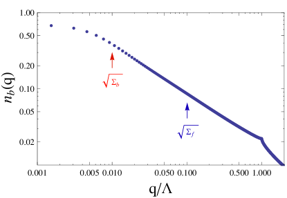
Figure 14: Momentum distribution $n_{b}(q)$ (Fourier transform of $A_{b}(x)$) in the fully localized phase. We have taken, $v_{f}/v_{b}=9$, $K_{b}=1.3$ and $g=0.4$. Also, $\hat{\Sigma}_{f}=0.01\Lambda$ and $\hat{\Sigma}_{b}=0.0001\Lambda$. Related momentum scales, $\sqrt{\hat{\Sigma}_{f}}$ and $\sqrt{\hat{\Sigma}_{b}}$ are pinpointed on the plot. Momentum $q$ is in unit of the UV cut-off $\Lambda$.

V Conclusion

Figure 15: Phase diagram of a 1D ⁸⁷Rb-⁴⁰K Bose-Fermi mixture, in the weak disorder limit. We consider an array of tubes, created with lasers of wavelength $\lambda$ = 755 nm, which corresponds to a (2D) lattice constant $d=\lambda/2$. We take $a_{bb}=100a_{0}$ as Bose-Bose scattering length, while the Bose-Fermi scattering length, $a_{bf}$, is tuned using a Feshbach resonance. The one.dimensional densities are chosen to be $\rho_{f}d=0.3$ and $\rho_{b}d=0.2$. The recoil energy is $E_{R,b}=h^{2}\lambda^{-2}/(2m_{Rb})$, while $V_{\perp b}$ is the transverse confining potential creating the 1D tubes. The Bose-Bose interaction $U_{b}$ increases with $V_{\perp b}$. Note that despite a superficial similarity between the present figure and, for instance, Fig. 6, the vertical axis is reverted, since $K_{b}$ decreases as $U_{b}$ increases. Four phases and the region of instability of the Luttinger liquid theory are shown. BFG: Bose-Fermi glass, BFG^∗ (BFG with an extremely large bosonic localization length), AG+SFB: Anderson Glass + Superfluid Bosons, LL: Luttinger liquid.

In this article, we have studied in detail a 1D mixture of bosons and fermions in a random potential. More precisely we have considered the localization of the gas by analyzing the pinning of density waves by weak disorder. In the case of incommensurate densities, to which we focused throughout this paper, the two components of the gas are coupled to Fourier components of the random potential that are effectively uncorrelated. The two density waves are, however, coupled through the Bose-Fermi interactions. Using renormalization group methods as well as a self-consistent harmonic approximation in replica space, we arrived at the following general conclusions:

- For weak disorder, the phase diagram can be plotted adequately as a function of two parameters, the Luttinger parameter $K_{b}$ for bosons, and the Bose-Fermi interaction parameter $U_{bf}$. The structure of the phase diagram and the properties of the phases depend on a third parameter, the ratio of sound velocities, $v_{f}/v_{b}$. Whatever the value of this ratio, we can identify three distinct phases, (i) a two-component Luttinger liquid, dominated by superfluid correlations for bosons and pair correlations for fermions, (ii) a fully localized phase where both components of the gas are pinned by disorder and (iii) an intermediate phase where fermions are localized and bosons are superfluid. In Fig. 15 we propose a translation of the diagram of Fig. 6 to microscopic parameters relevant for an experiment using a mixture of ⁸⁷Rb and ⁴⁰K Best et al. (2009). This translation is done along the lines detailed in Ref. Crépin et al., 2010.

Figure 16: The momentum distribution of bosons in the fully localized phase exhibits a saturation for momenta below $1/L_{b}$. Above this threshold, we identify a crossover between two algebraic regimes. Bosonic interactions are renormalized by Bose-Fermi interactions on length scales smaller than the fermionic localization length $L_{f}$. Indeed for $q>1/L_{f}$ the exponent of the power law is renormalized by BF interactions, while for $1/L_{b}<q<1/L_{f}$ the exponent is controlled by bare interactions.

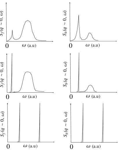
Figure 17: Sketch of the structure factor – for bosons and fermions – in the three phases identified in Fig.15. Top pannel: fully localizd phase, middel pannel: intermediate phase with localized fermions and superfluid bosons, bottom pannel: Luttinger liquid phase. The presence of two peaks in each phase is characteristic of the strong coupling between the two components of the gas, even in the localized phases. In the latter the widths of the peaks are inversely proportional to the localization lengths.

- The properties of the fully localized phase depend strongly on the strength of Bose-Fermi interactions as well as on the ratio of velocities. Both from the RG and from the variational calculations we conclude that this phase is characterized by two length scales, $L_{f}$ and $L_{b}$, which can be identified as the fermionic and bosonic localization lengths. Beyond these length scales the phase correlations of the density waves are lost. For strong Bose-Fermi interactions, these two length scales can be very different. In the case where $v_{f}>v_{b}$ (and for similar amplitudes of the disorder), $L_{b}$ is larger than $L_{f}$ for two reasons: first, because $K_{b}>K_{f}$ and therefore quantum fluctuations tend to suppress more strongly the pinning of the bosonic density wave, and second, because despite localization, fast fermionic phonons screen repulsive bosonic interactions and increase $L_{b}$ further. In the case $v_{b}>v_{f}$ on the other hand, the order of $L_{f}$ and $L_{b}$ can be reverted, because, quantum fluctuations through $K_{b}$ and the effective attractive interactions for the fermions have competing effects on localization.

- In any case, for a finite size system, it is likely that one of the localization length exceeds the size of the system. One of the species would then appear as delocalized. Also, finite temperature can overshadow the effects of disorder if the thermal length is comparable to one of the localization lengths.

Experimentally, the localization phase transition can be most easily observed in correlation functions, which uniquely depend on the phase. For the bosons, such a quantity is provided by the momentum distribution $n_{b}(q)$ of the quasi-condensate, which is directly measurable through time of flight (TOF) experiments. As shown in Fig. 14 and sketched in Fig. 16, there bosonic localization should simply be observed as a saturation of $n_{b}(q)$ at momenta smaller than $\sim 1/L_{b}$, provided temperature is low enough (if the thermal length $v_{b}/(k_{B}T)$ is smaller than $L_{b}$ then localization is obscured by thermal fluctuations).

Unfortunately, pure fermionic phase correlations are much more difficult to access. They appear as p-wave superconducting fluctuations, and would probably be only measurable through rather difficult noise correlation measurments. However, the fermionic localization does have an impact on $n_{b}(q)$ and should also be visible in the dynamical structure factor. Indeed we computed the latter quantity using our variational solution in replica space. As sketched in Fig.17, it can distinguish between localized and superfluid phases. Several key features are to be noted. First, the presence of two peaks in each phase is a direct consequence of the strong coupling – through Bose-Fermi interactions – between both componnents of the gas, even in the fully localized phase. Second, the width of the peaks in the localized phases is controlled by the inverse of the localization lengths. For the parameters of Fig. 15 where fermions are the fast component, $L_{b}\gg L_{f}$ in the fully localzed phase, and the bosonic peak is much sharper than its fermionic counterpart. In the intermediate phase, where bosons are superfluid it becomes a Dirac delta. Note that according to our analysis of the dynamical functions $I_{f}$ and $I_{b}$ – see equations (111) and (112) as well as (191) and (192)– in both localized phases the structure factor grows linearly at small frequencies. In the Luttinger liquid phase one should be able to retrieve the two sound modes from the peak positions, $\omega_{+}=v_{+}q$ and $\omega_{-}=v_{-}q$. One should also bear in mind that for non-zero $q$, deviations from the linear dispersion (assumed in a Luttinger liquid description) will lead to a broadening of these peaks. It then might be difficult to distinguish peaks from the Luttinger liquid phase and peaks from the localized phase in the case of very large localization lengths. The comparison will be easier for short localization lengths, a regime likely to be attained for either strong bosonic repulsions (Tonks-Girardeau regime) or small Bose-Fermi interactions.

Finally, we would like to point out that dynamical quantities are key observables to investigate the effects of the various levels of replica symmetry breaking. Here we computed the structure factors by making simple approximations for the dynamical parts of the self-energies. It remains to solve completely the system of self-consistent equations to obtain a definitive view on the structure factor, to go beyond the sketches presented in Fig. 17.

Appendix A Normal modes of the homogeneous Bose-Fermi mixture

Starting from the Hamiltonian of Eq. (II.1), one uses standard diagonalization methods to find:

$$H=\sum_{\alpha=\pm}\frac{v_{\alpha}}{2\pi}\int dx\left[K_{\alpha}\left(\nabla\theta_{\alpha}\right)^{2}+\frac{1}{K_{\alpha}}\left(\nabla\phi_{\alpha}\right)^{2}\right],$$ (119)

with $K_{\pm}=1$ and,

$$v_{\pm}^{2}=\frac{1}{2}(v_{f}^{2}+v_{b}^{2})\pm\frac{1}{2}\sqrt{(v_{f}^{2}-v_{b}^{2})^{2}+4g^{2}v_{f}^{2}v_{b}^{2}},$$ (120)

where $g=\frac{U_{bf}}{\pi}\sqrt{\frac{K_{f}K_{b}}{v_{f}v_{b}}}$ is a dimensionless parameter. Transformation rules betweenhe fields $(\phi_{f},\phi_{b})$ and $(\phi_{+},\phi_{-})$ are related as $\phi_{f}=f_{+}\phi_{+}+f_{-}\phi_{-}$, $\phi_{b}=b_{+}\phi_{+}+b_{-}\phi_{-}$, with the coefficients are defined as follows:

$$f_{+}=\sqrt{\frac{K_{f}v_{f}}{v_{+}}}\sin(\theta), \;\;f_{-}=\sqrt{\frac{K_{f}v_{f}}{v_{-}}}\cos(\theta),$$

$$b_{+}=\sqrt{\frac{K_{b}v_{b}}{v_{+}}}\cos(\theta), \;\;b_{-}=-\sqrt{\frac{K_{b}v_{b}}{v_{-}}}\sin(\theta).$$

A similar transformation relates $(\theta_{f},\theta_{b})$ to $(\theta_{+},\theta_{-})$, that is, $\theta_{f}=\bar{f}_{+}\theta_{+}+\bar{f}_{-}\theta_{-}$ and $\theta_{b}=\bar{b}_{+}\theta_{+}+\bar{b}_{-}\theta_{-}$. Coefficients for this transformation are:

$$\bar{f}_{+}=\sqrt{\frac{v_{+}}{K_{f}v_{f}}}\sin(\theta), \;\;\bar{f}_{-}=\sqrt{\frac{v_{-}}{K_{f}v_{f}}}\cos(\theta),$$

$$\bar{b}_{+}=\sqrt{\frac{v_{+}}{K_{b}v_{b}}}\cos(\theta), \;\;\bar{b}_{-}=-\sqrt{\frac{v_{-}}{K_{b}v_{b}}}\sin(\theta).$$

The rotation angle $\theta$ is defined by:

$$\cos(2\theta)=\frac{v_{b}^{2}-v_{f}^{2}}{v_{+}^{2}-v_{-}^{2}},\ \ \ \sin(2\theta)=\frac{2gv_{f}v_{b}}{v_{+}^{2}-v_{-}^{2}}$$ (121)

One can check that for $U_{bf}=g=0$

$$\left.\begin{array}[]{ll}f_{+}=\sqrt{K_{f}},&f_{-}=0,\\ b_{-}=\sqrt{K_{b}},&b_{+}=0,\\ v_{+}=v_{f},&v_{-}=v_{b}\end{array}\right\}\;\;\textrm{if}\ v_{f}>v_{b}\;,$$ (122)

$$\left.\begin{array}[]{lll}f_{+}=0,&f_{-}=\sqrt{K_{f}},\\ b_{-}=0,&b_{+}=\sqrt{K_{b}},\\ v_{+}=v_{f},&v_{-}=v_{b}\end{array}\right\}\;\;\textrm{if}\ v_{b}>v_{f}\;.$$ (123)

Appendix B RG calculation

The renormalization group (RG) relies upon the assumption that all important phenomena occur over length scales much larger than a microscopic length $\Lambda^{-1}$. In our case, we use a hydrodynamic theory, and $\Lambda^{-1}$ can be identified as the mean inter-particle distance, i.e., $\Lambda\sim\rho$, the mean density. At each RG step we integrate out high momentum excitations by reducing the cutoff $\Lambda\to\Lambda^{\prime}$, while renormalizing the parameters of the Hamiltonian – and possibly generating new couplings, and thereby generate an RG trajectory.

In a system with quenched disorder the thermodynamic quantity of interest is the average free energy $F$,

$$-\beta F=\overline{\log Z}\;.$$ (124)

Here $Z$ is the partition function for a given realization of the random potential, and $\overline{\phantom{i}\ldots\phantom{i}}$ denotes averaging over disorder. To compute (124) we use the so-called replica trick Mézard et al. (1987): we introduce $n$ identical copies of the system, average over the disorder and then take the limit $n\rightarrow 0$,

$$\lim\limits_{n\rightarrow 0}\frac{1}{n}\log\overline{Z^{n}}=\overline{\log Z}\;.$$ (125)

In pratice, we work with $\overline{Z^{n}}$ to perform the RG. Using a path integral formulation, the partition function $Z$ reads:

$$Z=\int D\phi_{f}D\phi_{b}\ e^{-S[\phi_{f},\phi_{b}]}\;.$$ (126)

Here the action $S=S_{0}+S_{\text{dis}}$ is given by Eqs. (52) and (53). Assuming that $\xi_{\alpha}$ are random functions with a Gaussian distribution, $P(\xi_{\alpha},\xi_{\alpha}^{*})=\exp[-D_{\alpha}^{-1}\int dx\ \xi_{\alpha}(x)\xi_{\alpha}(x)^{*}]$, we can compute $\overline{Z^{n}}$, and arrive at

$$\overline{Z^{n}} = \int\prod_{a=1}^{n}D\phi_{f}^{a}D\phi_{b}^{a}\ e^{-\sum\limits_{a=1}^{n}S_{0}[\phi_{f}^{a},\phi_{b}^{a}]/\hbar}\ \overline{e^{-\sum\limits_{a=1}^{n}S_{dis}[\phi_{f}^{a},\phi_{b}^{a}]/\hbar}}$$ (127)

$$= \int\prod_{a=1}^{n}D\phi_{f}^{a}D\phi_{b}^{a}\ e^{-\sum\limits_{a=1}^{n}S_{0}[\phi_{f}^{a},\phi_{b}^{a}]}\exp\left[\sum\limits_{\alpha=f,b}{D_{\alpha}\rho_{\alpha}^{2}}\sum\limits_{a,b=1}^{n}\int dxd\tau d\tau^{\prime}e^{i2\phi_{\alpha}^{a}(x,\tau)}e^{-i2\phi_{\alpha}^{b}(x,\tau^{\prime})}\right]$$

$$= \int\prod_{a=1}^{n}D\phi_{f}^{a}D\phi_{b}^{a}\ e^{-S_{\text{rep}}},$$

with the replicated action, $S_{\text{rep}}=S_{0}^{\text{rep}}+S_{\text{dis}}^{\text{rep}}$ defined through Eqs. (55) and (56).

To perform the RG calculation we introduce a UV cutoff $\Lambda$ on the momenta only, and write the fields $\phi_{f},\phi_{b}$ as well $\phi_{+}$ and $\phi_{-}$ as

$$\phi_{\alpha}(x,\tau)=\frac{1}{\beta L}\sum_{\underset{|q|<\Lambda}{q,\omega_{n}}}\phi_{\alpha}(q,\omega_{n})e^{iqx-i\omega_{n}\tau}\;.$$ (128)

Next, we introduce the slow and fast fields,

$$\phi_{\alpha}^{<}(x,\tau) = \frac{1}{\beta L}\sum_{\underset{|q|<\Lambda^{\prime}}{q,\omega_{n}}}\phi_{\alpha}(q,\omega_{n})e^{iqx-i\omega_{n}\tau},$$ (129)

$$\phi_{\alpha}^{>}(x,\tau) = \frac{1}{\beta L}\sum_{\underset{\Lambda^{\prime}<|q|<\Lambda}{q,\omega_{n}}}\phi_{\alpha}(q,\omega_{n})e^{iqx-i\omega_{n}\tau}\;,$$ (130)

and integrate out the fast fields to obtain

$$\overline{Z_{\Lambda}^{n}}=Z_{0}^{>}\int\prod_{a=1}^{n}D\phi_{f}^{a,<}D\phi_{b}^{a,<}e^{-S_{0}^{<}}\langle e^{-S_{\text{dis}}^{\text{rep}}}\rangle_{>}\;.$$ (131)

Performing then a cumulant expansion to first order in $D_{f}$ and $D_{b}$ we get

$$\langle e^{-S_{\text{dis}}^{\text{rep}}}\rangle_{>} \simeq \exp\left[\sum\limits_{\alpha=f,b}{D_{\alpha}\rho_{\alpha}^{2}}\sum\limits_{a=1}^{n}\int dxd\tau d\tau^{\prime}e^{i2\phi_{\alpha}^{a,<}(x,\tau)}e^{-i2\phi_{\alpha}^{a,<}(x,\tau^{\prime})}\langle e^{i2\phi_{\alpha}^{a,>}(x,\tau)}e^{-i2\phi_{\alpha}^{a,>}(x,\tau^{\prime})}\rangle_{>}\right]$$

$$= \exp\left[\sum\limits_{\alpha=f,b}{D_{\alpha}\rho_{\alpha}^{2}}\sum\limits_{a=1}^{n}\int dxd\tau d\tau^{\prime}e^{i2\phi_{\alpha}^{a,<}(x,\tau)}e^{-i2\phi_{\alpha}^{a,<}(x,\tau^{\prime})}\langle e^{i2\phi_{\alpha}^{a,>}(x,\tau)}\rangle_{>}^{2}\right.$$

$$+ \left.\sum\limits_{\alpha=f,b}{D_{\alpha}\rho_{\alpha}^{2}}\sum\limits_{a=1}^{n}\int dxd\tau d\tau^{\prime}e^{i2\phi_{\alpha}^{a,<}(x,\tau)}e^{-i2\phi_{\alpha}^{a,<}(x,\tau^{\prime})}\left[\langle e^{i2\phi_{\alpha}^{a,>}(x,\tau)}e^{-i2\phi_{\alpha}^{a,>}(x,\tau^{\prime})}\rangle_{>}-\langle e^{i2\phi_{\alpha}^{a,>}(x,\tau)}\rangle_{>}^{2}\right]\right].$$

Note that, to first order, every correlation functions appearing in (LABEL:eq:cumulant) is diagonal in replica space. Let us therefore drop the replica indices for the rest of this Section. Also, let us keep only $D_{f}$ for convenience. Using the normal modes $\phi_{+}$ and $\phi_{-}$, we find that: $\langle e^{i2\phi_{\alpha}^{>}(x,\tau)}\rangle_{>}^{2}=(\Lambda^{\prime}/\Lambda)^{2f_{+}^{2}+2f_{-}^{2}}$. Therefore the first term in the bracket of equation (B) reads

$$\frac{D_{f}\rho_{f}^{2}}{v_{f}^{2}\Lambda^{3}}\left(\frac{\Lambda^{\prime}}{\Lambda}\right)^{2f_{+}^{2}+2f_{-}^{2}}\Lambda^{3}\int dxd(v_{f}\tau)d(v_{f}\tau^{\prime})e^{i2\phi_{f}^{<}(x,\tau)}e^{-i2\phi_{f}^{<}(x,\tau^{\prime})}$$ (133)

$$=\tilde{D}_{f}\left(\frac{\Lambda^{\prime}}{\Lambda}\right)^{2f_{+}^{2}+2f_{-}^{2}-3}\Lambda^{\prime 3}\int dxd(v_{f}\tau)d(v_{f}\tau^{\prime})e^{i2\phi_{f}^{<}(x,\tau)}e^{-i2\phi_{f}^{<}(x,\tau^{\prime})}\;,$$ (134)

where we have defined the dimensionless coupling $\tilde{D}_{f}=\frac{D_{f}\rho_{f}^{2}}{v_{f}^{2}\Lambda^{3}}$. To preserve the low energy form of the action for a rescaled cutoff, $\Lambda^{\prime}$, one should rescale $\tilde{D}_{f}$ so that:

$$\tilde{D}_{f}(\Lambda^{\prime})=\tilde{D}_{f}(\Lambda)\left(\frac{\Lambda^{\prime}}{\Lambda}\right)^{2f_{+}^{2}+2f_{-}^{2}-3}.$$ (135)

Assuming an infinitesimal change of the cutoff, $\Lambda^{\prime}=\Lambda(1-dl)$, we obtain Eq. (57). Eq. (58) can be obtained i na similar way.

Let us now take care of the second bracket in equation (B). It contributes mainly when $\tau$ and $\tau^{\prime}$ are close, and will essentially renormalize the coefficient of $(\partial_{\tau}\phi_{f})^{2}$ in the quadratic action. First let us deal with:

$$\mathcal{A}=\langle e^{i2\phi_{f}^{>}(x,\tau)}e^{-i2\phi_{f}^{>}(x,\tau^{\prime})}\rangle_{>}-\langle e^{i2\phi_{f}^{>}(x,\tau)}\rangle_{>}^{2}.$$ (136)

We have:

$$\langle e^{i2\phi_{f}^{>}(x,\tau)}e^{-i2\phi_{f}^{>}(x,\tau^{\prime})}\rangle_{>}=e^{-\sum\limits_{\alpha=\pm}2f_{\alpha}^{2}\langle(\phi_{\alpha}(x,\tau)-\phi_{\alpha}(x,\tau^{\prime}))^{2}\rangle_{>}}$$

$$=\exp\Biggl{[}-\sum\limits_{\alpha=\pm}2f_{\alpha}^{2}\sum\limits_{\underset{\Lambda^{\prime}<|q|<\Lambda}{q,\omega_{n}}}[2-2\cos(\omega_{n}\bar{\tau})]\frac{\pi v_{\alpha}}{\omega_{n}^{2}+v_{\alpha}^{2}q^{2}}\Biggr{]}$$ (137)

with $\bar{\tau}=\tau-\tau^{\prime}$ and:

$$\langle e^{i2\phi_{f}^{>}(x,\tau)}\rangle_{>}^{2}=\exp\left[-\sum\limits_{\alpha=\pm}4f_{\alpha}^{2}\sum\limits_{\underset{\Lambda^{\prime}<|q|<\Lambda}{q,\omega_{n}}}\frac{\pi v_{\alpha}}{\omega_{n}^{2}+v_{\alpha}^{2}q^{2}}\right].$$ (138)

Then factorizing $\langle e^{i2\phi_{f}^{>}(x,\tau)}e^{-i2\phi_{f}^{>}(x,\tau^{\prime})}\rangle_{>}$ in $\mathcal{A}$ and using the fact that $\Lambda^{\prime}=\Lambda(1-dl)$, an expansion to first order in $dl$ leads to.

$$\mathcal{A}=\langle e^{i2\phi_{f}^{>}(x,\tau)}e^{-i2\phi_{f}^{>}(x,\tau^{\prime})}\rangle_{>}\sum_{\alpha=\pm}2f_{\alpha}^{2}e^{-v_{\alpha}|\bar{\tau}|\Lambda}dl.$$ (139)

We are left with:

$$\mathcal{B} = {D_{\alpha}\rho_{\alpha}^{2}}\int dxd\tau d\tau^{\prime}e^{i2\phi_{f}^{<}(x,\tau)}e^{-i2\phi_{f}^{<}(x,\tau^{\prime})}\mathcal{A}$$ (140)

$$= {D_{\alpha}\rho_{\alpha}^{2}}\int dxd\tau d\tau^{\prime}:e^{i2\phi_{f}^{<}(x,\tau)}e^{-i2\phi_{f}^{<}(x,\tau^{\prime})}:e^{-\sum\limits_{\alpha=\pm}2f_{\alpha}^{2}\int_{0}^{\Lambda}dq(1-e^{-v_{\alpha}|\bar{\tau}|q})/q}\sum_{\alpha=\pm}2f_{\alpha}^{2}e^{-v_{\alpha}|\bar{\tau}|\Lambda}dl.$$

:…: stands for normal-ordering. The function $\mathcal{G}(\bar{\tau})=\exp\left[-\sum\limits_{\alpha=\pm}2f_{\alpha}^{2}\int_{0}^{\Lambda}dq(1-e^{-v_{\alpha}|\bar{\tau}|q})/q\right]$ is obtained after taking the normal order and combining the extra factor $\langle e^{i2\phi_{f}^{<}(x,\tau)}e^{-i2\phi_{f}^{<}(x,\tau^{\prime})}\rangle_{<}$ with $\mathcal{A}$. Finally we expand the exponential in powers of $\bar{\tau}$:

$$\mathcal{B}\simeq-dl{D_{\alpha}\rho_{\alpha}^{2}}\left[\int dxdT(\partial_{T}\phi_{f})^{2}\right]\int d\bar{\tau}\bar{\tau}^{2}\mathcal{G}(\bar{\tau})$$

$$\times\sum_{\alpha=\pm}4f_{\alpha}^{2}e^{-v_{\alpha}|\bar{\tau}|\Lambda}$$ (141)

$\mathcal{G}(\bar{\tau})$ is easily evaluated to be:

$$\mathcal{G}(\bar{\tau})=\prod_{\alpha=\pm}(v_{\alpha}\Lambda|\bar{\tau}|)^{-2f_{\alpha}^{2}}e^{-2f_{\alpha}^{2}(\gamma+\Gamma(0,v_{\alpha}\Lambda|\bar{\tau}|)}$$ (142)

with $\gamma$ Euler’s constant and $\Gamma(0,z)$ the incomplete Gamma function. In the end we find that $\mathcal{B}$ can be cast into:

$$\mathcal{B}\simeq-dl\tilde{D}_{f}\left[f_{+}^{2}\mathcal{C}_{+}\frac{v_{f}^{2}}{v_{+}^{3}}\left(\frac{v_{+}}{v_{-}}\right)^{2f_{-}^{2}}+f_{-}^{2}\mathcal{C}_{-}\frac{v_{f}^{2}}{v_{-}^{3}}\left(\frac{v_{-}}{v_{+}}\right)^{2f_{+}^{2}}\right]$$ (143)

$$\times\left[\int dxdT(\partial_{T}\phi_{f})^{2}\right].$$

Here we have defined $\mathcal{C}_{\pm}(K_{b},K_{f},v_{f}/v_{b})$ as

$$\mathcal{C}_{+} = 8\int_{0}^{\infty}dzz^{2-X_{f}}e^{-2\gamma X_{f}}e^{-2f_{+}^{2}\Gamma(0,z)-2f_{-}^{2}\Gamma(0,\frac{v_{-}}{v_{+}}z)}\;,$$

$$\mathcal{C}_{-} = 8\int_{0}^{\infty}dzz^{2-X_{f}}e^{-2\gamma X_{f}}e^{-2f_{+}^{2}\Gamma(0,\frac{v_{+}}{v_{-}}z)-2f_{-}^{2}\Gamma(0,z)}\;.$$

Both $v_{f}$ and $K_{f}$ are renormalized by this term, and we find for the flow equations:

$$\frac{dK_{f}}{dl} = -\frac{K_{f}^{2}}{2}\tilde{D}_{f}\left[f_{+}^{2}\mathcal{C}_{+}\frac{v_{f}^{3}}{v_{+}^{3}}\left(\frac{v_{+}}{v_{-}}\right)^{2f_{-}^{2}}+f_{-}^{2}\mathcal{C}_{-}\frac{v_{f}^{3}}{v_{-}^{3}}\left(\frac{v_{-}}{v_{+}}\right)^{2f_{+}^{2}}\right],$$ (145)

$$\frac{dv_{f}}{dl} = -\frac{K_{f}^{2}}{2}v_{f}\tilde{D}_{f}\left[f_{+}^{2}\mathcal{C}_{+}\frac{v_{f}^{3}}{v_{+}^{3}}\left(\frac{v_{+}}{v_{-}}\right)^{2f_{-}^{2}}+f_{-}^{2}\mathcal{C}_{-}\frac{v_{f}^{3}}{v_{-}^{3}}\left(\frac{v_{-}}{v_{+}}\right)^{2f_{+}^{2}}\right].$$ (146)

These flow equations describe the phase transition for small but finite values of $\tilde{D}_{f}$ and $\tilde{D}_{b}$.

Appendix C Self-consistent equations for the RSB solutions

We start from the replicated action. The idea of the Gaussian variational method is to replace the complicated action $S$ by its best Gaussian approximation $S_{G}$:

$$S_{G}=\frac{1}{2}\frac{1}{\beta L}\sum_{q,i\omega_{n}}\phi_{\alpha}^{a}(q,i\omega_{n})(G^{-1})_{\alpha\beta}^{ab}(q,i\omega_{n})\phi_{\beta}^{b}(-q,-i\omega_{n}),$$

The propagator $G$ is a $2n\times 2n$ matrix with the following structure:

$$G^{-1}=\left(\begin{array}[]{ll}\left[G^{-1}\right]_{ff}^{ab}&\left[G^{-1}\right]_{fb}^{ab}\\ \left[G^{-1}\right]_{bf}^{ab}&\left[G^{-1}\right]_{bb}^{ab}\end{array}\right)$$ (147)

where $\left[G^{-1}\right]_{\alpha\beta}$, $\alpha,\beta=f,b$ is consequently a $n\times n$ matrix. Using the well-known inequality, $F\leq F_{\rm var}[G]\equiv F_{G}+\frac{1}{\beta}\langle S-S_{G}\rangle_{G}$, we can obtain an estimate for $F$ by minimizing the variational free energy $F_{var}$ with respect to $G$. Here $F_{G}=-\frac{1}{\beta}\log[\textrm{Tr}e^{-S_{G}}]$ is the Free energy of the Gaussian theory. The three terms, $F_{G}$, $\langle S_{0}\rangle_{G}$ and $\langle S_{\rm dis}\rangle_{G}$ can be easily computed to obtain

$$F_{var} = -\frac{1}{2\beta}\sum_{q,i\omega_{n}}\textrm{Tr}\log[G(q,i\omega_{n})]$$ (148)

$$+ \frac{1}{2}\sum_{\alpha,\beta}\sum_{q,i\omega_{n}}\left(G_{0}^{-1}\right)_{\alpha\beta}(q,i\omega_{n})\textrm{Tr}[G_{\alpha\beta}(q,i\omega_{n})]$$

$$+ \frac{1}{2}\sum_{a,b}L\int d\tau\left(V_{F}[F^{ab}(\tau)]+V_{B}[B^{ab}(\tau)]\right).$$

Here we have defined the two functions, $V_{F}$ and $V_{B}$, so that $V_{F}(x)=-2{\rho_{f}^{2}D_{f}}e^{-2x}$ and $V_{B}(x)=-2{\rho_{b}^{2}D_{b}}e^{-2x}$, and introduced

$$F^{ab}(\tau) \equiv G^{aa}_{ff}(0,0)+G^{bb}_{ff}(0,0)-2G^{ab}_{ff}(0,\tau),$$ (149)

$$B^{ab}(\tau) \equiv G^{aa}_{bb}(0,0)+G^{bb}_{bb}(0,0)-2G^{ab}_{bb}(0,\tau).$$ (150)

Notice that only the replica-diagonal elements, $F^{aa}(\tau)$ and $F^{bb}(\tau)$ turn out to be time-dependent, and the replica-offdiagonal elements, representing disorder-generated correlations between replicas are just constants in time. We now look for the saddle-point equations by differentiating $F_{var}$ with respect to $G$, and requiring $\delta F_{var}$=0. This yields

$$\left.\begin{array}[]{ll}(G^{-1})_{ff}^{ab}(q,i\omega_{n})&=-2\beta\delta_{n,0}V^{\prime}_{F}(F^{ab})\\ (G^{-1})_{bb}^{ab}(q,i\omega_{n})&=-2\beta\delta_{n,0}V^{\prime}_{B}(B^{ab})\end{array}\right\}\;\;\mbox{ a$\neq$ b},$$ (151)

with

$$\left.\begin{array}[]{ll}F^{ab}=\frac{1}{\beta L}\sum\limits_{q,i\omega_{n}}\left[G_{ff}^{aa}(q,i\omega_{n})+G_{ff}^{bb}(q,i\omega_{n})\right]-\frac{2}{\beta L}\sum\limits_{q}G_{ff}^{ab}(q,\omega_{n}=0)\\ \\ B^{ab}=\frac{1}{\beta L}\sum\limits_{q,i\omega_{n}}\left[G_{bb}^{aa}(q,i\omega_{n})+G_{bb}^{bb}(q,i\omega_{n})\right]-\frac{2}{\beta L}\sum\limits_{q}G_{bb}^{ab}(q,\omega_{n}=0)\end{array}\right\}\;\;\mbox{ a$\neq$ b},$$ (152)

and

$$(G^{-1})_{ff}^{aa}(q,i\omega_{n}) = (G_{0}^{-1})_{ff}(q,i\omega_{n})+2\int_{0}^{\beta}d\tau\left(1-\cos[\omega_{n}\tau]\right)V^{\prime}_{F}(F^{aa}(\tau))+2\int_{0}^{\beta}d\tau\sum_{b\neq a}V_{F}^{\prime}[F^{ab}],$$ (153)

$$(G^{-1})_{bb}^{aa}(q,i\omega_{n}) = (G_{0}^{-1})_{bb}(q,i\omega_{n})+2\int_{0}^{\beta}d\tau\left(1-\cos[\omega_{n}\tau]\right)V^{\prime}_{B}(B^{aa}(\tau))+2\int_{0}^{\beta}d\tau\sum_{b\neq a}V_{B}^{\prime}[B^{ab}].$$ (154)

We remark here that the matrix elements that mix species are unaffected by disorder:

$$(G^{-1})_{fb}^{ab}(q,i\omega_{n})=(G^{-1})_{bf}^{ab}(q,i\omega_{n})=(G_{0}^{-1})_{bf}(q,i\omega_{n})\delta_{a,b}\;.$$ (155)

We now take the limit $n\rightarrow 0$ and introduce Parisi’s parameterization for $0\times 0$ matrices.Marc Mézard and Giorgio Parisi (1991) Let $A$ be a matrix in replica space. Taking $n=0$, $A$ can be described by a couple $(\tilde{a},a(u))$ with $\tilde{a}$ corresponding to the diagonal elements of $A$, and $a(u)$ a function of $u\in[0,1]$, parameterizing the off-diagonal elements. For multiplication and inversion rules of Parisi matrices, see for example Ref. Marc Mézard and Giorgio Parisi, 1991.

With the Parisi parametrization, the previous equations read:

$$(G^{-1}(u))(q,\omega_{n})=-2\beta\delta_{n,0}\;\begin{pmatrix}V_{F}^{\prime}[F(u)]&0\\ 0&V_{B}^{\prime}[B(u)]\end{pmatrix}$$ (156)

and

$$\widetilde{G^{-1}}_{\alpha\beta}(q,\omega_{n})=(G^{-1}_{0})_{\alpha\beta}(q,\omega_{n})-\delta_{\alpha\beta}\Pi_{\alpha}(q,\omega_{n})\;,$$ (157)

with the fermionic ”self-energy” defined as

$$\Pi_{f}(q,\omega_{n}) = -2\int_{0}^{\beta}d\tau\left(1-\cos[\omega_{n}\tau]\right)V^{\prime}_{F}[\widetilde{F}(\tau)]+2\beta\int_{0}^{1}\,du\,V_{F}^{\prime}[F(u)]\;,$$ (158)

and the bosonic self-energy given by a similar expression. The replica-diagonal and off-diagonal parts of $F^{ab}$ then read

$$\widetilde{F}(\tau) \equiv 2\bigl{(}\widetilde{G}_{ff}(0,0)-\widetilde{G}_{ff}(0,\tau)\bigr{)}\;,$$

$$F(u) = \frac{2}{\beta L}\sum\limits_{q,i\omega_{n}}\left[\widetilde{G}_{ff}(q,i\omega_{n})-\delta_{\omega_{n},0}\,\widetilde{G}_{ff}(q,u)\right]\;,$$

and similar expressions hold for the functions $B(u)$ and $\widetilde{B}(\tau)$.

The connected Green’s function, more precisely its inverse, $(G^{-1})^{c}_{\alpha\beta}\equiv\sum\limits_{b}(G^{-1})^{ab}_{\alpha\beta}$, was already defined in the main text. Let us finally express this in terms of the Parisi parametrization,

$$(G^{-1})^{c}_{\alpha\beta}=\widetilde{G^{-1}}_{\alpha\beta}-\int_{0}^{1}du\ G^{-1}_{\alpha\beta}(u)\;.$$ (159)

The integral equations above need be solved self-consistently. However, as we shall see, they do not have a unique solution. Therefore, we need to supplement the above set of integral equations by yet another condition, which shall be the marginality condition of the replicon mode, discussed later.Giamarchi and Le Doussal (1996) Similar to other quantum glass phases, this condition turns out to yield physically meaningful solutions in all phases.Georges et al. (2001)

C.1 Level 1 RSB

To describe the phase with localized fermions and superfluid bosons, we assume a level one replica symmetry breaking in the fermionic sector, while the bosonic sector remains replica symmetric. To simplify notations, we introduce the self-energy

$$\sigma_{f}(u)=2\beta V_{F}^{\prime}[F(u)]\;.$$ (160)

Level one RSB implies that there exists a value $0<u_{f}<1$ such that $\sigma_{f}(u<u_{f})=0$ and $\sigma_{f}(u>u_{f})=\sigma_{f}$, or equivalently $F(u<u_{f})=\infty$ and $F(u>u_{f})=F$. The corresponding bosonic self-energy $\sigma_{b}(u)$ is identically zero in this phase. Then the matrix elements of $(G^{-1})^{c}_{\alpha\beta}$ read:

$$(G^{-1})^{c}_{ff} = (G_{0}^{-1})_{ff}(i\omega_{n},q)+I_{F}(\omega_{n})+\Sigma_{F}(1-\delta_{n,0})\;,$$

$$(G^{-1})^{c}_{bb} = (G_{0}^{-1})_{bb}(i\omega_{n},q)+I_{B}(\omega_{n})\;,$$

$$(G^{-1})^{c}_{fb} = (G^{-1})^{c}_{bf}=(G_{0}^{-1})_{fb}(i\omega_{n},q)\;,$$

with the functions $I_{B/F}(\omega_{n})$ defined as

$$I_{B}(\omega_{n}) = 2\int_{0}^{\beta}d\tau\left(1-\cos[\omega_{n}\tau]\right)V^{\prime}_{B}[\widetilde{B}(\tau)]\;,$$ (162)

$$I_{F}(\omega_{n}) = 2\int_{0}^{\beta}d\tau\left(1-\cos[\omega_{n}\tau]\right)\times$$ (163)

$$\hskip 28.45274pt\times(V^{\prime}_{F}[\widetilde{F}(\tau)]-V_{F}^{\prime}[F])\;,$$

and the ’mass’ $\Sigma_{F}$ given by

$$\Sigma_{f}=2\beta u_{f}V_{F}^{\prime}[F]\;.$$

To obtain the self-consistency equations for $\sigma_{f}$ and $I_{F},I_{B}$, one needs to invert the matrix $(G^{-1})_{\alpha\beta}$. This can be carried out using Parisi’s multiplication and inversion formulasMarc Mézard and Giorgio Parisi (1991), and we find:

$$F = \frac{2}{\beta L}\sum_{q,i\omega_{n}}\frac{\pi K_{f}}{v_{f}}\frac{\frac{\omega_{n}^{2}}{v_{b}^{2}}+q^{2}+\hat{I}_{b}(\omega_{n})}{\left(\frac{\omega_{n}^{2}}{v_{b}^{2}}+q^{2}+\hat{I}_{b}(\omega_{n})\right)\left(\frac{\omega_{n}^{2}}{v_{f}^{2}}+q^{2}+\hat{I}_{f}(\omega_{n})+\hat{\Sigma}_{f}\right)-g^{2}q^{4}}\;,$$ (164)

$$\widetilde{F}(\tau) = \frac{2}{\beta L}\sum_{q,i\omega_{n}}\frac{\pi K_{f}}{v_{f}}\left(1-\cos[\omega_{n}\tau]\right)\frac{\frac{\omega_{n}^{2}}{v_{b}^{2}}+q^{2}+\hat{I}_{b}(\omega_{n})}{\left(\frac{\omega_{n}^{2}}{v_{b}^{2}}+q^{2}+\hat{I}_{b}(\omega_{n})\right)\left(\frac{\omega_{n}^{2}}{v_{f}^{2}}+q^{2}+\hat{I}_{f}(\omega_{n})+\hat{\Sigma}_{f}\right)-g^{2}q^{4}}\;,$$ (165)

$$\widetilde{B}(\tau) = \frac{2}{\beta L}\sum_{q,i\omega_{n}}\frac{\pi K_{b}}{v_{b}}\left(1-\cos[\omega_{n}\tau]\right)\frac{\frac{\omega_{n}^{2}}{v_{f}^{2}}+q^{2}+\hat{I}_{f}(\omega_{n})+\hat{\Sigma}_{f}}{\left(\frac{\omega_{n}^{2}}{v_{b}^{2}}+q^{2}+\hat{I}_{b}(\omega_{n})\right)\left(\frac{\omega_{n}^{2}}{v_{f}^{2}}+q^{2}+\hat{I}_{f}(\omega_{n})+\hat{\Sigma}_{f}\right)-g^{2}q^{4}}\;.$$ (166)

Here we have introduced $\hat{I}_{f}=\frac{\pi K_{f}}{v_{f}}I_{F}$, $\hat{\Sigma}_{F}=\frac{\pi K_{f}}{v_{f}}\Sigma_{F}$, and used similar notations for bosons. One can check that $B$ is indeed infinity. The self-consistent set of equations can be cast into:

$$\hat{\Sigma}_{F} = 2\beta\frac{\pi K_{f}}{v_{f}}u_{f}V^{\prime}_{F}[F],$$

$$\hat{I}_{f}(\omega_{n}) = 2\frac{\pi K_{f}}{v_{f}}\int_{0}^{\beta}d\tau\left(1-\cos[\omega_{n}\tau]\right)(V^{\prime}_{F}[\widetilde{F}(\tau)]-V_{F}^{\prime}[F]),$$

$$\hat{I}_{b}(\omega_{n}) = 2\frac{\pi K_{b}}{v_{b}}\int_{0}^{\beta}d\tau\left(1-\cos[\omega_{n}\tau]\right)V^{\prime}_{B}[\widetilde{B}(\tau)].$$ (167)

However, these equations do not determine the break point, $u_{f}$. The value of the latter can be determined using the so-called marginality condition on the replicon mode Giamarchi and Le Doussal (1996). We expand the variational free energy to second order, around the saddle-point. To do so, we write $G(q,i\omega_{n})=G^{(0)}(q,i\omega_{n})+g(q)$, where $G^{(0)}$ denotes the saddle-point solution, and and $G^{(0)}$ (as well as $g(q)$) is a Parisi matrix with matrix elements

$$[G^{(0)}]^{-1}(i\omega_{n}=0,q)=\left(\begin{array}[]{cc}(\widetilde{\Gamma}_{f},\Gamma_{f}(u))&(\widetilde{\Gamma}_{fb},0)\\ (\widetilde{\Gamma}_{fb},0)&(\widetilde{\Gamma}_{b},0)\end{array}\right)\;.$$ (168)

In a similar way:

$$g(q)=\left(\begin{array}[]{cc}(0,g_{f}(q,u))&(0,g_{fb}(q,u))\\ (0,g_{bf}(q,u))&(0,g_{b}(q,u))\end{array}\right)$$ (169)

Note that since the RSB only happens for the $\omega_{n}=0$ mode, we only need to perturb that particular mode. We then expand $F_{\rm var}$ up to second order in $g(q)$, yielding

$$\delta^{2}F_{var}=\frac{1}{4\beta}\sum_{q}\textrm{Tr}\left[[G^{(0)}(q)]^{-1}g(q)\right]^{2}\\ -n\frac{1}{\beta L}\int_{0}^{1}du\sum_{q,q^{\prime}}\left[g_{f}(q,u)g_{f}(q^{\prime},u)V_{F}^{\prime\prime}[F(u)]+g_{b}(q,u)g_{b}(q^{\prime},u)V_{B}^{\prime\prime}[B(u)]\right].$$

This can be written as $\delta^{2}F_{var}=\sum\limits_{q,q^{\prime}}\int\limits_{0}^{1}du\int\limits_{0}^{1}du^{\prime}[g]^{T}(q,u)M(q,q^{\prime},u,u^{\prime})[g](q,u)$, with $[g]^{T}=[g_{f},g_{b},g_{fb},g_{bf}]$. The stability matrix $M$ greatly simplifies if $g(q,u)$ is a so-called replicon mode, for which $\int_{0}^{u_{f}}du\ g(u)=0$ and $\int_{u_{f}}^{1}du\ g(u)=0$. In this case we find a symmetrical stability matrix, which, after introducing the notation $\langle\Gamma_{f}\rangle=\int_{0}^{1}du\Gamma_{f}(u)$, takes the form

$$M^{(u<u_{f})\;}(q,q^{\prime},u,u^{\prime})=-\frac{1}{4\beta}\delta(u-u^{\prime})\left(\begin{array}[]{cccc}(\widetilde{\Gamma}_{f}-\langle\Gamma_{f}\rangle)^{2}\delta_{qq^{\prime}}&\widetilde{\Gamma}_{fb}^{2}\delta_{qq^{\prime}}&(\widetilde{\Gamma}_{f}-\langle\Gamma_{f}\rangle)\widetilde{\Gamma}_{fb}\delta_{qq^{\prime}}&(\widetilde{\Gamma}_{f}-\langle\Gamma_{f}\rangle)\widetilde{\Gamma}_{fb}\delta_{qq^{\prime}}\\ \star&\widetilde{\Gamma}_{b}^{2}\delta_{qq^{\prime}}&\widetilde{\Gamma}_{b}\widetilde{\Gamma}_{fb}\delta_{qq^{\prime}}&\widetilde{\Gamma}_{b}\widetilde{\Gamma}_{fb}\delta_{qq^{\prime}}\\ \star&\star&\widetilde{\Gamma}_{fb}^{2}\delta_{qq^{\prime}}&(\widetilde{\Gamma}_{f}-\langle\Gamma_{f}\rangle)\widetilde{\Gamma}_{b}\delta_{qq^{\prime}}\\ \star&\star&\star&\widetilde{\Gamma}_{fb}^{2}\delta_{qq^{\prime}}\end{array}\right)\;,$$ (170)

$$M^{(u>u_{f})\;}(q,q^{\prime},u,u^{\prime})=-\frac{1}{4\beta}\delta(u-u^{\prime})\left(\begin{array}[]{cccc}(\widetilde{\Gamma}_{f}-\Gamma_{f})^{2}\delta_{qq^{\prime}}+\frac{4}{L}V_{F}^{\prime\prime}[F]&\widetilde{\Gamma}_{fb}^{2}\delta_{qq^{\prime}}&(\widetilde{\Gamma}_{f}-\Gamma_{f})\widetilde{\Gamma}_{fb}\delta_{qq^{\prime}}&(\widetilde{\Gamma}_{f}-\Gamma_{f})\widetilde{\Gamma}_{fb}\delta_{qq^{\prime}}\\ \star&\widetilde{\Gamma}_{b}^{2}\delta_{qq^{\prime}}&\widetilde{\Gamma}_{b}\widetilde{\Gamma}_{fb}\delta_{qq^{\prime}}&\widetilde{\Gamma}_{b}\widetilde{\Gamma}_{fb}\delta_{qq^{\prime}}\\ \star&\star&\widetilde{\Gamma}_{fb}^{2}\delta_{qq^{\prime}}&(\widetilde{\Gamma}_{f}-\Gamma_{f})\widetilde{\Gamma}_{b}\delta_{qq^{\prime}}\\ \star&\star&\star&\widetilde{\Gamma}_{fb}^{2}\delta_{qq^{\prime}}\end{array}\right)\;,$$ (171)

and the marginality condition is $\sum\limits_{q^{\prime}}M(q,q^{\prime},u,u)[g(q^{\prime},u)]=0$. For $u<u_{f}$ this is trivially satisfied, while for $u>u_{f}$ it leads to the following condition:

$$-\frac{4}{L}\left(\frac{\pi K_{f}}{v_{f}}\right)^{2}V_{F}^{\prime\prime}(F)\sum_{q}\frac{1}{\left[q^{2}(1-g^{2})+\hat{\Sigma}_{f}\right]^{2}}=1\;,$$ (172)

which becomes for $L\rightarrow\infty$,

$$\hat{\Sigma}_{f}^{3/2}=-\left(\frac{\pi K_{f}}{v_{f}}\right)^{2}\frac{V_{F}^{\prime\prime}(F)}{\sqrt{1-g^{2}}}\;,$$ (173)

and closes the system of self-consistent equations.

C.2 Level 2 RSB

To describe the fully localized phase, we assume replica symmetry breaking in both the fermionic and the bosonic sectors. It turns out that one cannot reach a self-consistent set of equations with a level 1 RSB in each sector, however, it is sufficient to assume a level 2 RSB in one of the sectors, and a level 1 RSB in the other one. We proceed along the same path as before, excepting that now there are two break points, $u_{1}$ and $u_{2}$, such that

$$\sigma_{f}(u<u_{1}) = 0,$$

$$\sigma_{f}(u_{1}<u<u_{2}) = \sigma_{f}^{(1)}\equiv 2\beta V_{F}^{\prime}[F^{(1)}],$$

$$\sigma_{f}(u_{2}<u<1) = \sigma_{f}^{(2)}\equiv 2\beta V_{F}^{\prime}[F^{(2)}],$$

$$\sigma_{b}(u<u_{2}) = 0,$$

$$\sigma_{b}(u_{2}<u<1) = \sigma_{b}^{(2)}\equiv 2\beta V_{B}^{\prime}[B^{(2)}].$$ (174)

Now we have:

$$\hat{I}_{f}(\omega_{n}) = 2\frac{\pi K_{f}}{v_{f}}\int_{0}^{\beta}d\tau\left(1-\cos[\omega_{n}\tau]\right)(V^{\prime}_{F}[\widetilde{F}(\tau)]-V_{F}^{\prime}[F^{(2)}]),$$

$$\hat{I}_{b}(\omega_{n}) = 2\frac{\pi K_{b}}{v_{b}}\int_{0}^{\beta}d\tau\left(1-\cos[\omega_{n}\tau]\right)(V^{\prime}_{B}[\widetilde{B}(\tau)]-V_{B}^{\prime}[B^{(2)}]),$$

$$\hat{\Sigma}_{F} = 2\beta\frac{\pi K_{f}}{v_{f}}\left[u_{1}V^{\prime}_{F}[F^{(1)}]+u_{2}\left(V^{\prime}_{F}[F^{(2)}]-V^{\prime}_{F}[F^{(1)}]\right)\right],$$

$$\hat{\Sigma}_{B} = 2\beta\frac{\pi K_{b}}{v_{b}}u_{2}V^{\prime}_{B}[B^{(2)}]$$ (175)

The inversion of the propagator leads to:

$$B^{(2)} = \frac{2}{\beta L}\sum_{q,i\omega_{n}}\frac{\pi K_{b}}{v_{b}}\frac{\frac{\omega_{n}^{2}}{v_{f}^{2}}+q^{2}+\hat{I}_{f}(\omega_{n})+\hat{\Sigma}_{F}}{\left(\frac{\omega_{n}^{2}}{v_{b}^{2}}+q^{2}+\hat{I}_{b}(\omega_{n})\right)\left(\frac{\omega_{n}^{2}}{v_{f}^{2}}+q^{2}+\hat{I}_{f}(\omega_{n})+\hat{\Sigma}_{f}\right)-g^{2}q^{4}}$$ (176)

$$F^{(2)} = \frac{2}{\beta L}\sum_{q,i\omega_{n}}\frac{\pi K_{f}}{v_{f}}\frac{\frac{\omega_{n}^{2}}{v_{b}^{2}}+q^{2}+\hat{I}_{b}(\omega_{n})+\hat{\Sigma}_{B}}{\left(\frac{\omega_{n}^{2}}{v_{b}^{2}}+q^{2}+\hat{I}_{b}(\omega_{n})\right)\left(\frac{\omega_{n}^{2}}{v_{f}^{2}}+q^{2}+\hat{I}_{f}(\omega_{n})+\hat{\Sigma}_{f}\right)-g^{2}q^{4}}$$ (177)

$$F^{(2)}-F^{(1)} = -2\pi\frac{K_{f}}{v_{f}}\frac{1}{u_{2}\beta L}\sum_{q}\frac{(q^{2}+\hat{\Sigma}_{B})\Delta\hat{\Sigma}_{F}^{(2)}+g^{2}q^{2}\Sigma_{B}}{\left((q^{2}+\hat{\Sigma}_{B})(q^{2}+\hat{\Sigma}_{F})-g^{2}q^{4}\right)\left(q^{2}(1-g^{2})+\hat{\Sigma}_{F}^{(1)}\right)}$$ (178)

where we have introduced $\Delta\hat{\Sigma}_{F}^{(2)}=2\beta\frac{\pi K_{f}}{v_{f}}u_{2}\left(V^{\prime}_{F}[F^{(2)}]-V^{\prime}_{F}[F^{(1)}]\right)$ and $\hat{\Sigma}_{F}^{(1)}=2\beta\frac{\pi K_{f}}{v_{f}}u_{1}V^{\prime}_{F}[F^{(1)}]$ – so that $\hat{\Sigma}_{F}=\hat{\Sigma}_{F}^{(1)}+\Delta\hat{\Sigma}_{F}^{(2)}$. As in the previous section we need two more equations to find $u_{1}$ and $u_{2}$ and close the system. We also look for the marginality condition of the replicon mode, which we define as a mode satisfying $\int\limits_{u_{1}}^{u_{2}}du\ g(u)\equiv 0$ and $\int\limits_{u_{2}}^{1}du\ g(u)\equiv 0$. Now the stability matrix reads: $\bullet$ for $u<u_{1}$,

$$M(q,q^{\prime},u,u^{\prime})=-\frac{1}{4\beta}\delta(u-u^{\prime})\left(\begin{array}[]{cccc}(\widetilde{\Gamma}_{f}-\langle\Gamma_{f}\rangle)^{2}\delta_{qq^{\prime}}&\widetilde{\Gamma}_{fb}^{2}\delta_{qq^{\prime}}&(\widetilde{\Gamma}_{f}-\langle\Gamma_{f}\rangle)\widetilde{\Gamma}_{fb}\delta_{qq^{\prime}}&(\widetilde{\Gamma}_{f}-\langle\Gamma_{f}\rangle)\widetilde{\Gamma}_{fb}\delta_{qq^{\prime}}\\ \star&(\widetilde{\Gamma}_{b}-\langle\Gamma_{b}\rangle)^{2}\delta_{qq^{\prime}}&(\widetilde{\Gamma}_{b}-\langle\Gamma_{b}\rangle)\widetilde{\Gamma}_{fb}\delta_{qq^{\prime}}&(\widetilde{\Gamma}_{b}-\langle\Gamma_{b}\rangle)\widetilde{\Gamma}_{fb}\delta_{qq^{\prime}}\\ \star&\star&\widetilde{\Gamma}_{fb}^{2}\delta_{qq^{\prime}}&(\widetilde{\Gamma}_{f}-\langle\Gamma_{f}\rangle)(\widetilde{\Gamma}_{b}-\langle\Gamma_{b}\rangle)\delta_{qq^{\prime}}\\ \star&\star&\star&\widetilde{\Gamma}_{fb}^{2}\delta_{qq^{\prime}}\end{array}\right)\;,$$

$\bullet$ for $u_{1}<u<u_{2}$,

$$\left(\begin{array}[]{cccc}\left(\widetilde{\Gamma}_{f}-\Gamma_{f}^{(2)}+\Delta\Gamma_{f}^{(2)}\right)^{2}\delta_{qq^{\prime}}+\frac{4}{L}V_{F}^{\prime\prime}[F^{(1)}]&\widetilde{\Gamma}_{fb}^{2}\delta_{qq^{\prime}}&\left(\widetilde{\Gamma}_{f}-\Gamma_{f}^{(2)}+\Delta\Gamma_{f}^{(2)}\right)\widetilde{\Gamma}_{fb}\delta_{qq^{\prime}}&\left(\widetilde{\Gamma}_{f}-\Gamma_{f}^{(2)}+\Delta\Gamma_{f}^{(2)}\right)\widetilde{\Gamma}_{fb}\delta_{qq^{\prime}}\\ \star&(\widetilde{\Gamma}_{b}-\langle\Gamma_{b}\rangle)^{2}\delta_{qq^{\prime}}&(\widetilde{\Gamma}_{b}-\langle\Gamma_{b}\rangle)\widetilde{\Gamma}_{fb}\delta_{qq^{\prime}}&(\widetilde{\Gamma}_{b}-\langle\Gamma_{b}\rangle)\widetilde{\Gamma}_{fb}\delta_{qq^{\prime}}\\ \star&\star&\widetilde{\Gamma}_{fb}^{2}\delta_{qq^{\prime}}&\left(\widetilde{\Gamma}_{f}-\Gamma_{f}^{(2)}+\Delta\Gamma_{f}^{(2)}\right)(\widetilde{\Gamma}_{b}-\langle\Gamma_{b}\rangle)\delta_{qq^{\prime}}\\ \star&\star&\star&\widetilde{\Gamma}_{fb}^{2}\delta_{qq^{\prime}}\end{array}\right)\;,$$

$\bullet$ for $u_{2}<u<1$,

$$\left(\begin{array}[]{cccc}(\widetilde{\Gamma}_{f}-\Gamma_{f}^{(2)})^{2}\delta_{qq^{\prime}}+\frac{4}{L}V_{F}^{\prime\prime}[F^{(2)}]&\widetilde{\Gamma}_{fb}^{2}\delta_{qq^{\prime}}&(\widetilde{\Gamma}_{f}-\Gamma_{f}^{(2)})\widetilde{\Gamma}_{fb}\delta_{qq^{\prime}}&(\widetilde{\Gamma}_{f}-\Gamma_{f}^{(2)})\widetilde{\Gamma}_{fb}\delta_{qq^{\prime}}\\ \star&(\widetilde{\Gamma}_{b}-\Gamma_{b}^{(2)})^{2}\delta_{qq^{\prime}}+\frac{4}{L}V_{B}^{\prime\prime}[B^{(2)}]&(\widetilde{\Gamma}_{b}-\Gamma_{b}^{(2)})\widetilde{\Gamma}_{fb}\delta_{qq^{\prime}}&(\widetilde{\Gamma}_{b}-\Gamma_{b}^{(2)})\widetilde{\Gamma}_{fb}\delta_{qq^{\prime}}\\ \star&\star&\widetilde{\Gamma}_{fb}^{2}\delta_{qq^{\prime}}&(\widetilde{\Gamma}_{f}-\Gamma_{f}^{(2)})(\widetilde{\Gamma}_{b}-\Gamma_{b}^{(2)})\delta_{qq^{\prime}}\\ \star&\star&\star&\widetilde{\Gamma}_{fb}^{2}\delta_{qq^{\prime}}\end{array}\right)\;.$$

As before, on the first interval the marginality condition gives a trivial condition. On the second interval it gives:

$$-\frac{4}{L}\left(\frac{\pi K_{f}}{v_{f}}\right)^{2}V_{F}^{\prime\prime}[F^{(1)}]\sum_{q}\frac{1}{\left[q^{2}(1-g^{2})+\hat{\Sigma}_{f}^{(1)}\right]^{2}}=1,$$ (179)

and on the third we obtain:

$$\left[4\left(\frac{\pi K_{f}}{v_{f}}\right)^{2}V_{F}^{\prime\prime}[F^{(2)}]\ A_{ff}+1\right]\left[4\left(\frac{\pi K_{f}}{v_{f}}\right)^{2}V_{B}^{\prime\prime}[B^{(2)}]\ A_{bb}+1\right]=16\ \left(\frac{\pi K_{f}}{v_{f}}\right)^{2}\left(\frac{\pi K_{b}}{v_{b}}\right)^{2}V_{F}^{\prime\prime}[F^{(2)}]V_{B}^{\prime\prime}[B^{(2)}]\ A_{fb}^{2}\;,$$

with:

$$A_{ff} = \frac{1}{L}\sum_{q}\frac{\left(q^{2}+\hat{\Sigma}_{b}\right)^{2}}{\left[\left(q^{2}+\hat{\Sigma}_{f}\right)\left(q^{2}+\hat{\Sigma}_{b}\right)-g^{2}q^{4}\right]^{2}}\;,$$

$$A_{bb} = \frac{1}{L}\sum_{q}\frac{\left(q^{2}+\hat{\Sigma}_{f}\right)^{2}}{\left[\left(q^{2}+\hat{\Sigma}_{f}\right)\left(q^{2}+\hat{\Sigma}_{b}\right)-g^{2}q^{4}\right]^{2}}\;,$$

$$A_{fb} = \frac{1}{L}\sum_{q}\frac{\pi^{2}g^{2}q^{4}}{\left[\left(q^{2}+\hat{\Sigma}_{f}\right)\left(q^{2}+\hat{\Sigma}_{b}\right)-g^{2}q^{4}\right]^{2}}\;.$$

These conditions effectively close the system of self-consistent equations.

Appendix D Computation of the structure factor from the variational solution

As stated in the main text – see equation (110) – the structure factor for fermions is given by

$$S_{f}({q},\omega)=-\textrm{Im}\left[q^{2}\widetilde{G}_{ff}(q,i\omega_{n}\to\omega+i\epsilon)\right],$$ (180)

and we have a similar expression for bosons. Here, $\widetilde{G}_{ff(bb)}$ is the replica-diagonal contribution for the fermion (boson) propagator. We recall their expressions in the three phases. In the Luttinger liquid phase,

$$\widetilde{G_{ff}}(q,\omega_{n}) = \frac{\pi K_{f}}{v_{f}}\frac{q^{2}+b(\omega_{n})}{[q^{2}+b(\omega_{n})][q^{2}+f(\omega_{n})]-g^{2}q^{4}},$$

$$\widetilde{G_{bb}}(q,\omega_{n}) = \frac{\pi K_{b}}{v_{b}}\frac{q^{2}+b(\omega_{n})}{[q^{2}+f(\omega_{n})][q^{2}+f(\omega_{n})]-g^{2}q^{4}}.$$

Remember we have introduced the following general notation

$$b(\omega_{n}) = \omega_{n}^{2}/v_{b}^{2}+\hat{I}_{b}(\omega_{n})+\hat{\Sigma}_{b}\;,$$ (183)

$$f(\omega_{n}) = \omega_{n}^{2}/v_{f}^{2}+\hat{I}_{f}(\omega_{n})+\hat{\Sigma}_{f}\;.$$ (184)

In the Luttinger liquid phase $\hat{\Sigma}_{f}=\hat{\Sigma}_{b}=0$. In the phase where fermions are localized and bosons superfluid, the propagators read

$$\widetilde{G_{ff}}(q,\omega_{n}) = \frac{\pi K_{f}}{v_{f}}\Biggl{(}\frac{q^{2}+b(\omega_{n})}{[q^{2}+b(\omega_{n})][q^{2}+f(\omega_{n})]-g^{2}q^{4}}$$ (185)

$$+ \delta_{n,0}\frac{1}{1-g^{2}}\frac{\sigma_{f}}{q^{2}[q^{2}(1-g^{2})+\hat{\Sigma}_{f}]}\Biggr{)}\;,$$

$$\widetilde{G_{bb}}(q,\omega_{n}) = \frac{\pi K_{b}}{v_{b}}\Biggl{(}\frac{q^{2}+f(\omega_{n})}{[q^{2}+b(\omega_{n})][q^{2}+f(\omega_{n})]-g^{2}q^{4}}$$ (186)

$$+ \delta_{n,0}\frac{g^{2}}{1-g^{2}}\frac{\sigma_{f}}{q^{2}[q^{2}(1-g^{2})+\hat{\Sigma}_{f}]}\Biggr{)}\;.$$

Finally we add here the expressions of the propagators in the fully localized phase (for clarity they do not appear in the main text). They are

$$\widetilde{G_{ff}}(q,\omega_{n}) = \frac{\pi K_{f}}{v_{f}}\left.\frac{q^{2}+b(\omega_{n})}{[q^{2}+b(\omega_{n})][q^{2}+f(\omega_{n})]-g^{2}q^{4}}\right.$$

$$+ \delta_{n,0}\frac{\pi K_{f}}{v_{f}}\left[\frac{1}{1-g^{2}}\frac{\sigma_{f}^{(1)}}{q^{2}[q^{2}(1-g^{2})+\hat{\Sigma}_{f}^{(1)}]}\right.$$

$$+ \left.\frac{(\hat{\Sigma}_{b}+q^{2})\Delta\hat{\sigma}_{f}^{(2)}+q^{2}g^{2}\hat{\sigma}_{b}}{[q^{2}(1-g^{2})+\hat{\Sigma}_{f}^{(1)}][(q^{2}+\hat{\Sigma}_{f})(q^{2}+\hat{\Sigma}_{b})-g^{2}q^{4}]}\right],$$

$$\widetilde{G_{bb}}(q,\omega_{n}) = \frac{\pi K_{b}}{v_{b}}\frac{q^{2}+f(\omega_{n})}{[q^{2}+b(\omega_{n})][q^{2}+f(\omega_{n})]-g^{2}q^{4}}$$

$$+ \delta_{n,0}\frac{\pi K_{b}}{v_{b}}\frac{\sigma_{b}^{(2)}}{1-g^{2}}\frac{q^{2}+\hat{\Sigma}_{f}}{q^{2}[(q^{2}+\hat{\Sigma}_{f})(q^{2}+\hat{\Sigma}_{b})-g^{2}q^{4}]}$$

$$+ \ \delta_{n,0}\frac{\pi K_{b}}{v_{b}}\frac{g^{2}}{1-g^{2}}\left[\frac{\sigma_{f}^{(1)}}{q^{2}[q^{2}(1-g^{2})+\hat{\Sigma}_{f}^{(1)}]}\right.$$

$$+ \left.\frac{(\hat{\Sigma}_{f}+q^{2})\hat{\sigma}_{b}^{(2)}+q^{2}\Delta\hat{\sigma}_{f}^{(2)}}{[q^{2}(1-g^{2})+\hat{\Sigma}_{f}^{(1)}][(q^{2}+\hat{\Sigma}_{f})(q^{2}+\hat{\Sigma}_{b})-g^{2}q^{4}]}\right].$$

After the analytical continuation, the $\delta_{n,0}$ do not contribute and $\widetilde{G}_{ff}(q,\omega_{+})$ and $\widetilde{G}_{bb}(q,\omega_{+})$, with $\omega_{+}=\omega+i\epsilon$, are of the general form

$$\widetilde{G_{ff}}(q,-i\omega_{+}) = \frac{\pi K_{f}}{v_{f}}\frac{q^{2}+b(-i\omega_{+})}{[q^{2}+b(-i\omega_{+})][q^{2}+f(-i\omega_{+})]-g^{2}q^{4}},$$

$$\widetilde{G_{bb}}(q,-i\omega_{+}) = \frac{\pi K_{b}}{v_{b}}\frac{q^{2}+b(-i\omega_{+})}{[q^{2}+f(-i\omega_{+})][q^{2}+f(-i\omega_{+})]-g^{2}q^{4}}.$$

To get a useful form we introduce real and imaginary parts of $\hat{I}_{f}(-i\omega_{+})$ and $\hat{I}_{b}(-i\omega_{+})$ as $\hat{I}_{f}(-i\omega_{+})=\hat{I}_{f}^{\prime}(\omega)+i\hat{I}_{f}^{\prime\prime}(\omega)$ and $\hat{I}_{b}(-i\omega_{+})=\hat{I}_{b}^{\prime}(\omega)+i\hat{I}_{b}^{\prime\prime}(\omega)$. Finally we find for the structure factors

$$S_{f}(q,\omega) = -\frac{K_{f}}{\pi v_{f}}q^{2}\frac{\hat{I}_{f}^{\prime\prime}(\omega)\mathcal{P}_{b}(q,\omega)^{2}+\hat{I}_{b}^{\prime\prime}(\omega)\mathcal{P}_{fb}(q,\omega)}{\left[\hat{I}_{f}^{\prime\prime}(\omega)\mathcal{P}_{b}(q,\omega)+\hat{I}_{b}^{\prime\prime}(\omega)\mathcal{P}_{f}(q,\omega)\right]^{2}+\big{[}\mathcal{P}_{fb}(q,\omega)-\mathcal{P}_{f}(q,\omega)\mathcal{P}_{b}(q,\omega)\big{]}^{2}},$$ (191)

$$S_{b}(q,\omega) = -\frac{K_{b}}{\pi v_{b}}q^{2}\frac{\hat{I}_{b}^{\prime\prime}(\omega)\mathcal{P}_{f}(q,\omega)^{2}+\hat{I}_{f}^{\prime\prime}(\omega)\mathcal{P}_{fb}(q,\omega)}{\left[\hat{I}_{f}^{\prime\prime}(\omega)\mathcal{P}_{b}(q,\omega)+\hat{I}_{b}^{\prime\prime}(\omega)\mathcal{P}_{f}(q,\omega)\right]^{2}+\left[\mathcal{P}_{fb}(q,\omega)-\mathcal{P}_{f}(q,\omega)\mathcal{P}_{b}(q,\omega)\right]^{2}},$$ (192)

with

$$\mathcal{P}_{b}(q,\omega) = q^{2}+\hat{\Sigma}_{b}-\frac{\omega^{2}}{v_{b}^{2}}+\hat{I}_{b}^{\prime}(\omega),$$ (193)

$$\mathcal{P}_{f}(q,\omega) = q^{2}+\hat{\Sigma}_{f}-\frac{\omega^{2}}{v_{f}^{2}}+\hat{I}_{f}^{\prime}(\omega),$$ (194)

$$\mathcal{P}_{fb}(q,\omega) = \hat{I}_{f}^{\prime\prime}(\omega)\hat{I}_{b}^{\prime\prime}(\omega)+g^{2}q^{4}.$$ (195)

Remember that $\hat{I}_{f}^{\prime},\hat{I}_{f}^{\prime\prime},\hat{I}_{b}^{\prime},\hat{I}_{b}^{\prime\prime},\hat{\Sigma}_{f},\hat{\Sigma}_{b}$ depend on the phase one considers. Although for weak disorder the functions $\hat{I}_{f}$ and $\hat{I}_{b}$ might alter the dynamics only weakly, probing the dynamics would be a good way to test the effect of different levels of replica symmetry breaking. Note that according to (111) and (112), the sructure factors grow linearly at small frequency in the localized phases.