Anomalous critical behaviour in the polymer collapse transition of three-dimensional lattice trails

Abstract

Trails (bond-avoiding walks) provide an alternative lattice model of polymers to self-avoiding walks, and adding self-interaction at multiply visited sites gives a model of polymer collapse. Recently, a two-dimensional model (triangular lattice) where doubly and triply visited sites are given different weights was shown to display a rich phase diagram with first and second order collapse separated by a multi-critical point. A kinetic growth process of trails (KGT) was conjectured to map precisely to this multi-critical point. Two types of low temperature phases, globule and crystal-like, were encountered.

Here, we investigate the collapse properties of a similar extended model of interacting lattice trails on the simple cubic lattice with separate weights for doubly and triply visited sites. Again we find first and second order collapse transitions dependent on the relative sizes of the doubly and triply visited energies. However we find no evidence of a low temperature crystal-like phase with only the globular phase in existence.

Intriguingly, when the ratio of the energies is precisely that which separates the first order from the second-order regions anomalous finite-sized scaling appears. At the finite size location of the rounded transition clear evidence exists for a first order transition that persists in the thermodynamic limit. This location moves as the length increases, with its limit apparently at the point that maps to a KGT. However, if one fixes the temperature to sit at exactly this KGT point then only a critical point can be deduced from the data. The resolution of this apparent contradiction lies in the breaking of crossover scaling and the difference in the shift and transition width (crossover) exponents.

I Introduction

The canonical lattice model of the configurations of a polymer in solution has been the self-avoiding walk (SAW) where configurations are those lattice paths that could be generated by a random walk on a lattice that is not allowed to visit the same lattice site more than once. Considered as a static equilibrium statistical mechanical ensemble, self-avoiding walks display an excluded volume effect: they are swollen in size if compared to the set of unrestricted random walks of the same length. A common way to model intra-polymer interactions is to assign an energy to each non-consecutive pair of monomers lying on neighbouring lattice sites. This prescription defines the interacting self-avoiding walk (ISAW) model, which is the standard lattice model of polymer collapse using self-avoiding walks. The collapse transition in ISAW models, the so-called $\theta$-point of polymers, is a second order phase transition that has been well studied. The standard theory de Gennes (1975); Stephen (1975); Duplantier (1982) of the collapse transition is based on the $n\rightarrow 0$ limit of the magnetic tri-critical $\phi^{4}-\phi^{6}$ O($n$) field theory and related Edwards model with two and three body forces Duplantier (1986, 1987), which predicts an upper critical dimension of three with subtle scaling behaviour in that dimension.

A physically equivalent way of obtaining the excluded volume in a random walk model is to prevent the walk from visiting the same bond more than once. This weaker restriction leads to another class of lattice paths called self-avoiding trails (SAT). The interacting version of trails, customarily obtained by giving a weight to multiply occupied sites, also presents a collapse transition. The literature contains various definitions Meirovitch and Lim (1990); Prellberg (2001); Prellberg and Owczarek (2001) of single energy models of interacting self-avoiding trails (ISAT), all weighting multiply visited sites in different ways (they differ in how sites visited more than twice are assigned the energy of interaction). Regardless, theoretical prediction Shapir and Oono (1984) and the evidence Lim et al. (1988); Owczarek and Prellberg (1995); Prellberg and Owczarek (1995); Owczarek and Prellberg (2006) suggests that the collapse transition of the ISAT model is in a different universality class to that of ISAW, although there is no clear understanding of why this is the case if true.

On the other hand, a two-dimensional model (triangular lattice) of an extended ISAT (eISAT) model, where doubly and triply visited sites are given different energies, say $-\varepsilon_{2}$ and $-\varepsilon_{3}$ respectively, was recently Doukas et al. (2010) shown to display a rich phase diagram with first and second order collapse separated by a multi-critical point. The occurrence of the type of transition depended on the ratio

$$k=\frac{\varepsilon_{3}}{\varepsilon_{2}}$$ (1)

of the energies given to multiply visited sites of different degree.

In conjunction with this study a stochastic process, known as kinetic growth trails (KGT), was also considered, where configurations of trails are produced by a growth process. The static configurations produced are trails, but the trails of a fixed length are not all produced with equal probability. The equivalent static model is an eISAT with a particular value of $k=k_{G}\simeq 4.15$ at one particular temperature $T=T_{G}$. It was demonstrated Doukas et al. (2010) that this value of $k=k_{G}$ separates models where the collapse transition is first order ($k>k_{G}$) from models where the collapse transition is second order ($k<k_{G}$). It was shown that for $k<k_{G}$ the second order transition was most likely in a single universality class, which was the same as the one in the (two-dimensional) ISAW $\theta$-point collapse transition. Moreover, the KGT process mapped exactly onto the transition point separating the two lines of first and second order transition. Defining the temperature of the transition in the eISAT model to be $T_{c}(k)$, it was deduced that

$$T_{c}(k_{G})=T_{G}\;.$$ (2)

Also, importantly it was found that while the second order transition encountered for small $k$ had a low temperature phase that was globular, the low temperature phase at large $k$ was crystal-like, in that the trail filled the lattice.

In this paper we investigate a counterpart to the triangular lattice eISAT model on the simple cubic lattice. One reason for choosing the simple cubic lattice is that the coordination number is the same as on the triangular lattice. This means that if one considers a kinetic growth process KGT on the simple cubic lattice it will map to precisely that same location in the phase diagram of the three-dimensional model as the corresponding triangular lattice model described above. Also the KGT on the simple cubic lattice has previously been studied Prellberg and Owczarek (1995): it demonstrates a scaling behaviour consistent with it mapping to a critical point in the phase diagram of eISAT. One might then speculate that the phase diagram of the eISAT on the cubic lattice has the same structure as on the triangular lattice. However, we find there are important differences, including anomalous finite size scaling behaviour around the KGT point, and no evidence of any crystal-like low temperature phase.

The paper is set out as follows. We begin by recalling the theoretical framework of the collapse transition. We then move onto defining the models including the extended ISAT (eISAT) model on a general regular lattice, specifically on the triangular and cubic lattices, the various canonical ISAT models and the KGT process. Before describing our results for the cubic lattice we summarise the findings on the triangular lattice.

II Collapse Transition and Crossover Scaling

There are two related ways of describing the collapse. One is by understanding the change in finite length $n$ scaling of key quantities such as the radius of gyration, or alternatively end-to-end distance, and partition function as the temperature is lowered past the transition temperature $T_{c}$. The second is the associated singular thermodynamic behaviour in the thermodynamic limit ($n\to\infty$) of the free energy per step and in the internal energy and/or specific heat at that same temperature.

Let us first describe the finite size scaling change. As the temperature is varied there is a collapse transition at some $T=T_{c}$. For high temperatures ($T>T_{c}$) the excluded volume interaction is the dominant effect, and the behaviour is universally the same as the non-interacting SAW problem. The mean squared end-to-end distance $R_{n}^{2}$ and partition function $Z_{n}$ are therefore expected to scale as

$$R_{n}^{2} \sim A\,n^{2\nu}\qquad\mbox{with }\quad\nu>1/2,$$ (3)

$$Z_{n} \sim B\,\mu^{n}n^{\gamma-1}.$$

respectively with estimates of $\nu$ and $\gamma$ to be $0.5874(2)$ Prellberg (2001) and $1.156957(9)$ Clisby et al. (2007) in three dimensions.

When fixed at the transition temperature $T=T_{c}$ for ISAW in three dimensions, tri-critical field theory and the Edwards model Duplantier (1986, 1987) predict similar scaling forms with $\nu=1/2$ and $\gamma=1$, though with additive logarithmic corrections.

At low temperatures ($T>T_{c}$) it is accepted that the partition function is dominated by configurations that are internally dense. The partition function should then scale differently to that at high temperature, since a collapsed polymer should have a well defined surface (and associated surface energy). One expects Owczarek et al. (1993) in three dimensions asymptotics of the form

$$R_{n}^{2} \sim A\,n^{2/3},$$ (4)

$$Z_{n} \sim B\,\mu^{n}\mu_{s}^{n^{2/3}}n^{\gamma-1}.$$

with $\mu_{s}<1$. So the exponent $\nu=1/3$ and the fractal dimension of the polymer becomes $3$.

This change in scaling behaviour is reflected in the thermodynamic limit. In the thermodynamic limit there is expected to be a singularity in the free energy, which can be seen in its second derivative (the specific heat). Denoting the (intensive) finite length specific heat per monomer by $c_{n}(T)$, the thermodynamic limit is given by the long length limit as

$$C(T)=\lim_{n\rightarrow\infty}c_{n}(T)\;.$$ (5)

In general one expects that the singular part of the specific heat behaves as

$$C(T)\sim B|T_{c}-T|^{-\alpha}\;,$$ (6)

where $\alpha<1$ for a second-order phase transition. The singular part of the thermodynamic limit internal energy behaves as

$$U(T)\sim B|T_{c}-T|^{1-\alpha}\;,$$ (7)

if the transition is second-order, and there is a jump in the internal energy if the transition is first-order (an effective value of $\alpha=1$).

Moreover one expects crossover scaling forms Brak et al. (1993) to apply around this temperature, so that

$$c_{n}(T)\sim n^{\alpha\phi}\,\mathcal{C}([T-T_{c}]n^{\phi}),$$ (8)

with $0<\phi<1$ if the transition is second-order and

$$c_{n}(T)\sim n\;{\cal C}([T-T_{c}]n)$$ (9)

if the transition is first-order (that is, $\phi$ is effectively 1). Assuming standard crossover theory Lawrie and Sarbach (1984) it was deduced in Brak et al. (1993) that the exponents $\alpha$ and $\phi$ are related via

$$2-\alpha=\frac{1}{\phi}\;.$$ (10)

Regardless of whether the full crossover theory holds one can usually define an exponent $\psi$ from the shift of the transition temperature at finite length $T_{c,n}$ measured by, say, finding the position of a peak in the specific heat as follows

$$T_{c,n}-T_{c}\sim D\,n^{-\psi}.$$ (11)

Another exponent can be related to the width $\Delta T_{n}$ of the transition. We shall define this exponent $\phi$, via

$$\Delta T_{n}\sim E\,n^{-\phi}.$$ (12)

We use the same symbol $\phi$ because in a crossover theory the exponent will be the same $\phi$ as described in (8). For a first order transition one expects that both $\phi$ and $\psi$ are 1. For a second order transition in the standard scaling picture one expects the two exponents to be equal, $\psi=\phi$, although we note a breaking down of the standard scaling has been already observed in Prellberg and Owczarek (2002) in high dimensions.

For the ISAW model the tri-critical field theory expects the width (crossover) exponent $\phi=1/2$ and shift exponent $\psi=1/2$ with logarithmic corrections present in the scaling forms because the system is at the upper critical dimension. The value of the specific heat exponent $\alpha=0$ is consistent with the scaling relation (10), as a logarithmically divergent specific heat Duplantier (1986, 1987) is predicted,

$$c_{n}(T_{c})\sim C(\ln n)^{3/11}.$$ (13)

The prediction Duplantier (1986, 1987) for the shift is

$$T_{c,n}-T_{c}\sim D\,n^{-1/2}(\ln n)^{-7/11}.$$ (14)

On the other hand Shapir and Oono Shapir and Oono (1984) have argued that the ISAT collapse transition should be tri-critical in nature, as self-avoiding walks. However they predict that ISAW and ISAT are in different universality classes. Importantly, while the upper critical dimension for ISAW is expected to be $d_{u}=3$, the Shapir-Oono field theory gives $d_{u}=4$ for ISAT.

III Models

III.1 The general extended ISAT model (eISAT)

On a lattice with coordination number greater than 3 the self-interaction in the trail model can be implemented in different ways, depending on how the weight associated with contact site depends on how many times the site has been visited. The canonical ISAT model, which has been defined differently by different authors, fixes the energy associated with sites visited more than twice based upon the energy of doubly visited sites. The eISAT is a generalised model that allows for different (independent) energies to be associated with multiply visited sites of different multiplicities.

Consider a regular lattice of coordination number $2q$ $(q\in\mathbb{N},q\geq 2)$ and the configurations $\phi_{n}\in\Omega_{n}$ of trails of length $n$ (bonds) starting from a fixed origin. Let $-\varepsilon_{\ell}$ be the energy associated with lattice sites that have been visited $\ell$ times by the trail. Now let $m_{\ell},\ \ell=1,\dotsc q$ be the number of lattice sites that have been visited $\ell$ times by the trail. Note that one always has $\sum_{\ell}\,\ell\,m_{\ell}=n+1$. Hence, to each of these contact sites is associated an Boltzmann weight $\omega_{\ell}=e^{\beta\varepsilon_{\ell}}$ with $\omega_{1}=1$, where $\beta=1/T$ is the inverse temperature in suitable units of the inverse Boltzmann constant. The partition function is then given by:

$$Z_{n}(\omega_{2},\dotsc,\omega_{q})=\sum_{\phi_{n}\in\Omega_{n}}\omega_{2}^{m_{2}(\phi_{n})}\dotsm\omega_{q}^{m_{q}(\phi_{n})},$$ (15)

and the probability distribution by

$$p_{E}(\phi_{n};\omega_{2},\dotsc,\omega_{q})=\frac{\omega_{2}^{m_{2}(\phi_{n})}\dotsm\omega_{q}^{m_{q}(\phi_{n})}}{Z_{n}(\omega_{2},\dotsc,\omega_{q})}.$$ (16)

We define a reduced finite-size free energy per step as

$$\kappa_{n}=\frac{1}{n}\log Z_{n},$$ (17)

related to the usual free energy per step as $-\beta f_{n}=\kappa_{n}$.

The average of any quantity $Q$ over the ensemble of allowed paths $\phi_{n}\in\Omega_{n}$ of length $n$ is given generically by

$$\big{\langle}Q\big{\rangle}_{n}=\frac{1}{Z_{n}}\sum_{\phi_{n}\in\Omega_{n}}Q(\phi_{n})\ \omega_{2}^{m_{2}(\phi_{n})}\dotsm\omega_{q}^{m_{q}(\phi_{n})}.$$ (18)

The thermodynamic limit in this problem is given by the limit $n\to\infty$, so that the thermodynamic free energy per step $f_{\infty}$ is given by

$$-\beta f_{\infty}=\kappa_{\infty}=\lim_{n\to\infty}\kappa_{n}.$$ (19)

This quantity determines the asymptotic behaviour of the partition function, i.e., $Z_{n}$ grows to leading order exponentially as $\mu^{n}$ with $\mu=\exp\kappa_{\infty}$.

III.2 Cubic and triangular lattice eISAT

Both the triangular and simple cubic lattices have coordination number 6. Therefore only two weights, $\omega_{2}$ and $\omega_{3}$, appear in the formulae (15) and (16).

In order to explore the two-parameter space of the eISAT we define a one-parameter family of models with weights defined by:

$$(\omega_{2},\,\omega_{3})=(\omega,\omega^{k})\qquad\text{($k$-eISAT)}$$ (20)

for any positive real value of the parameter $k$, that is, the energies obey

$$\varepsilon_{3}=k\varepsilon_{2}$$ (21)

in the $k$-eISAT model. We set the energy $\varepsilon_{2}=1$ for convenience from now on.

In this parametrisation we define a reduced internal energy per step and a reduced specific heat per step in the usual way via

$$u_{n} =\partial\kappa_{n}/\partial\log\omega=\frac{\big{\langle}m_{2}+k\,m_{3}\big{\rangle}_{n}}{n}$$ (22)

$$c_{n} =\partial u_{n}/\partial\log\omega=\frac{\big{\langle}(m_{2}+k\,m_{3})^{2}\big{\rangle}_{n}-\big{\langle}m_{2}+k\,m_{3}\big{\rangle}_{n}^{2}}{n}.$$ (23)

Let us define the collapse transition as occurring at

$$\omega=\omega_{c}(k)$$ (24)

so that we expect for fixed $k$ that

$$c_{n}(\omega)\sim n^{\alpha\phi}\mathcal{C}((\omega-\omega_{c})n^{\phi}),$$ (25)

if crossover scaling occurs. More generally the shift exponent is defined by

$$\omega_{c,n}-\omega_{c}\sim D\,n^{-\psi},$$ (26)

where $\omega_{c,n}$ is the location of the peak of the specific heat, and the width exponent by

$$\Delta\omega_{n}\sim E\,n^{-\phi},$$ (27)

where $\Delta\omega_{n}$ is the width of the half-height of the peak of the specific heat. Both these exponents could depend on $k$.

III.3 “Canonical” ISAT models

The canonical model used by Doukas et al. Doukas et al. (2010) is one where every successive visit to a site adds an energy $-\varepsilon$ to the total for that site so that a $q$-times visited sites has energy $-(q-1)\varepsilon$. Therefore the canonical model is defined by the weight parametrisation

$$(\omega_{2},\omega_{3})=(\omega,\omega^{2})\;.$$ (28)

The canonical model corresponds to the case $k=2$ in our family of interacting trails.

A second “canonical” model used by Prellberg and Owczarek Prellberg and Owczarek (1995, 2001) has $k=3$ so that

$$(\omega_{2},\omega_{3})=(\omega,\omega^{3})\;.$$ (29)

In fact it seems that Meirovitch et al. Meirovitch and Lim (1990) used $\omega_{3}=\omega_{2}$, that is $k=1$. Interestingly, all these models $k=1,2,3$ have been seen Doukas et al. (2010) to behave in the same way on the triangular lattice and, as we shall see, seem to behave in the same way on the simple cubic lattice (though the two- and three-dimensional models differ from each other in behaviour).

III.4 Phase diagram of eISAT on the triangular lattice

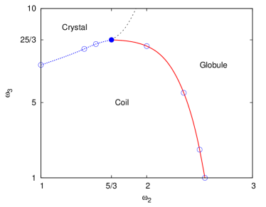
Figure 1: Phase diagram of eISAT on the triangular lattice. The dashed transition line for small $\omega_{2}$ (large $k$) separating the coil from the crystal-like phases represents a first-order transition and ends at the solid circle which is the kinetic growth point (KGT). This KGT point is conjectured to be multi-critical. The solid line separating the coil from the globule represents the $\theta$-like second order transition found for small $k$. The line separating the globule from the crystal-like phase is conjectured to be second order but not $\theta$-like.

The study by Doukas et al. Doukas et al. (2010) on the triangular lattice identified the kinetic growth point with a multi-critical collapse transition, being the meeting point of a swollen (coil), a collapsed and a crystal-like phase (see Fig. 1).

For small $\omega_{2}$ and $\omega_{3}$ the trails present the usual swollen polymer phase where $\nu=3/4$ (in two dimensions). For large enough $\omega_{2}$, regardless of $\omega_{3}$, there is a collapse phase, as occurs in the ISAW model, and a transition between the swollen and collapsed globule phases which seems to be $\theta$-like, with $\phi=3/7$ as expected in two dimensions. On the other hand, for large enough $\omega_{3}$ the ensemble is dominated by crystal-like configurations that are space filling and internally contain only triply-visited sites. Between the swollen phase and the crystal-like phase the collapse transition is first-order. Separating this line of first-order transitions from the line of $\theta$-like transitions is a multi-critical point. This point is precisely the point $(\omega^{*}_{2},\omega^{*}_{3})$ to which the kinetic growth process of trails maps. The crystal-like and globule phase is separated by a strong second order transition, much stronger than the $\theta$-collapse.

IV The kinetic growth process (KGT)

We now revisit the kinetic growth process Lyklema (1985) of trails (KGT). Consider a regular lattice of coordination number $2q$ $(q\in\mathbb{N})$, and consider a stochastic process defined as follows: starting at the origin, a lattice path is built up step-by-step by choosing between available continuing steps from unoccupied lattice bonds with equal probability. This dynamic process produces lattice paths that are self-avoiding trails, moreover it is easy to show that, on a coordination 6 lattice, a trail $\phi_{n}$ of length $n$ is generated with probability

$$p_{G}(\phi_{n})=\frac{1}{6}\left(\frac{1}{5}\right)^{n-1}\left(\frac{5}{3}\right)^{m_{2}(\phi_{n})}\left(\frac{25}{3}\right)^{m_{3}(\phi_{n})}.$$ (30)

This has to be compared with the probability distribution (16) of the equilibrium model with weights $(5/3,25/3)$

$$p_{E}\left(\phi_{n};\frac{5}{3},\frac{25}{3}\right)=\frac{1}{Z_{n}(\frac{5}{3},\frac{25}{3})}\left(\frac{5}{3}\right)^{m_{2}(\phi_{n})}\left(\frac{25}{3}\right)^{m_{3}(\phi_{n})},$$ (31)

from which we can deduce

$$p_{G}(\phi_{n})\propto p_{E}\left(\phi_{n};\frac{5}{3},\frac{25}{3}\right).$$ (32)

Note that the normalisation is different since the sum over all walks of fixed length gives the probability of walks being still open in the case of the growth process, and unity in the case of the equilibrium model.

We shall refer to the weight choice to which the KGT maps to as the Kinetic Growth point in the $(\omega_{2},\omega_{3})$ plane:

$$(\omega^{*}_{2},\omega^{*}_{3})=\left(\frac{5}{3},\frac{25}{3}\right)\qquad\text{(KGT)}.$$ (33)

The Kinetic Growth point does not correspond to any point in any of the canonical parametrisations described above (III.3) but it belongs to our family of interacting trails (20) with $k$ equal to

$$k_{G}\equiv\frac{\log 25/3}{\log 5/3}\simeq 4.15\ldots\;.$$ (34)

The KGT point has

$$T_{G}\equiv\frac{1}{\log 5/3}\simeq 1.957\dots\;.$$ (35)

In order to match the definition in (22) at the KGT point,

$${u}_{n}(\omega^{*}_{2},\omega^{*}_{3}) ={u}_{n}^{*}$$ (36)

$${c}_{n}(\omega^{*}_{2},\omega^{*}_{3}) ={c}_{n}^{*},$$ (37)

we define analogues of the internal energy and specific heat by

$${u}_{n}^{*} =\frac{\big{\langle}m_{2}+k_{G}\,m_{3}\big{\rangle}_{n}}{n}$$ (38)

$${c}_{n}^{*} =\frac{\big{\langle}(m_{2}+k_{G}\,m_{3})^{2}\big{\rangle}_{n}-\big{\langle}m_{2}+k_{G}\,m_{3}\big{\rangle}_{n}^{2}}{n}.$$ (39)

Kinetic Growth trails have been subject of various studies both in low and high dimensionality and on a variety of lattices (see, for example, Owczarek and Prellberg (1995); Prellberg and Owczarek (1995); Doukas et al. (2010)).

Simulations on the simple cubic lattice show a divergent specific heat with a logarithmic divergence different from the one predicted by the Edwards model.

In particular it was seen that

$${c}_{n}^{*}\sim C^{*}(\log n)^{\zeta}$$ (40)

with

$$\zeta=1.0\pm 0.5.$$ (41)

whereas the Edwards model has $\zeta=3/11$.

V Results for the cubic lattice eISAT

V.1 The KGT point

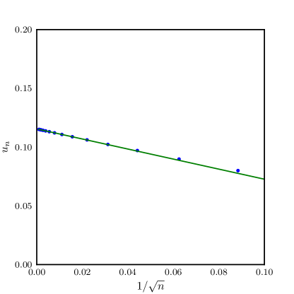
Figure 2: Plot of the energy $u_{n}$ of kinetic growth trails on the simple cubic lattice against $1/\sqrt{n}$, along with a line of best fit.

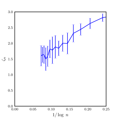
Figure 3: Estimating the exponent $\zeta$ in Eqn. (44) for KGT: Local slopes $\zeta_{n}$ of $\log c_{n}$ versus $\log\log n$ plotted against $1/\log n$. Error bars are obtained by a simple re-binning procedure.

We begin our investigation by revisiting the KGT point on the simple cubic lattice directly by simulating the eISAT at that point. That is, we have simulated the KGT point of the eISAT model at

$$(\omega_{2},\omega_{3})=(\omega^{*}_{2},\omega^{*}_{3})\equiv\left(\frac{5}{3},\frac{25}{3}\right)\;.$$ (42)

We simulated $10^{5}$ realisations of the kinetic growth process collecting $8.7\times 10^{4}$ samples of length $2^{20}$. We then computed the energy $u_{n}$ and the specific heat $c_{n}$. The results confirm what already was reported in Prellberg and Owczarek (1995): $u_{n}$ behaves as

$$u_{n}\sim u_{\infty}-\frac{u}{\sqrt{n}}\;,$$ (43)

as indicated in Fig. 2, and the specific heat $c_{n}$ diverges as a power of $\log n$

$$c_{n}\sim c\,(\log n)^{\zeta}.$$ (44)

We calculated the local slopes $\zeta_{n}$ of $\log c_{n}$ versus $\log\log n$, which are plotted versus $1/\log n$ in Fig. 3. We estimate $\zeta\simeq 1.0\pm 0.5$ as reported in Prellberg and Owczarek (1995).

V.2 The $k_{G}$-eISAT model

We have first simulated the $k$-eISAT model (20) with $k=k_{G}$ (the correspondence with KGT occurs at $\omega=5/3$) using the flatPERM algorithm Prellberg and Krawczyk (2004); Janse van Rensburg (2009). We ran $S=10^{5}$ iterations of generating about $S_{n}\simeq 9\cdot 10^{9}$ samples at length $10^{3}$. Following Prellberg and Krawczyk (2004), we also measured the number of samples adjusted by the number of their independent growth steps, obtaining $S_{n}^{eff}\simeq 4\cdot 10^{7}$ “effective” samples.

FlatPERM outputs an estimate $W_{n,m}$ of the total weight of the walks of length $n$ and fixed value of $m$. From the total weight one can access physical quantities over a broad range of temperatures through a simple weighted average, e.g.

$$u_{n}(\omega) =\frac{\sum_{m}m\,W_{n,m}}{\sum_{m}W_{n,m}}\quad\text{and}$$ (45)

$$c_{n}(\omega) =\frac{\sum_{m}m^{2}\,W_{n,m}}{\sum_{m}W_{n,m}}-\left(\frac{\sum_{m}m\,W_{n,m}}{\sum_{m}W_{n,m}}\right)^{2}\;.$$ (46)

The analysis of the scaling of the specific heat peak is done by calculating the location of the peak of the specific heat $\omega_{c,n}$ and thereby evaluating $c_{n}^{peak}=c_{n}(\omega_{c,n})$.

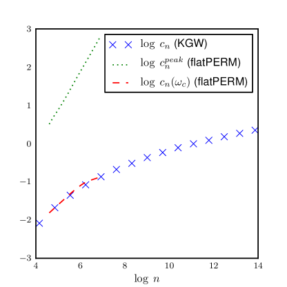
Figure 4: Comparison of the growth of the specific heat at the kinetic growth point (lower dashes and crosses) with the growth of the peak of the specific heat (upper dots) for eISAT with $k=k_{G}$. One clearly sees different growth rates in the upper and lower curves, in particular the peak of the specific heat (upper dots) grows linearly on this logarithmic scale.

At the kinetic growth point, we confirm the slow growth of the specific heat seen in the previous section (c.f. Eqn. (44)). The KGT simulations and flatPERM simulations evaluated at $\omega_{c}$ coincide as shown in Fig. 4.

Somewhat unexpectedly, the height of the peak of the specific heat, $c^{peak}_{n}$, shows a different behaviour, diverging as a power of $n$, as illustrated by the top curve in Fig. 4. In fact the divergence is linear, which indicates a first order transition. The nature of the finite-size transition is therefore very different from the one inferred from the kinetic growth process.

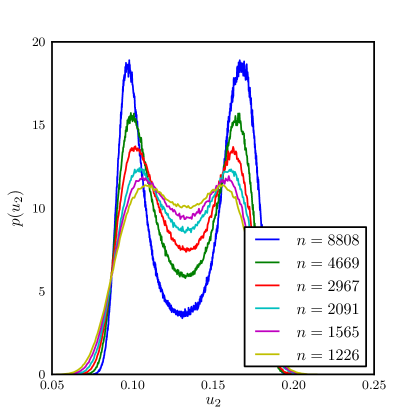
Figure 5: Normalised energy density of states near the kinetic-growth point for eISAT with $k=k_{G}$. The values of $\omega$ have been chosen such that both peaks have equal height. One clearly sees the build-up of a first-order transition with a well defined gap between the two peaks. This will result in a latent heat in the thermodynamic limit.

We have therefore simulated this model at longer lengths ($10^{4}$) using a thermal implementation of flatPERM at several fixed temperatures around the expected location of the transition. We have found that the energy distribution shows indeed a double peak (see Fig. 5) with the two peaks getting more and more definite as the length scale increases.

We infer from this that a simulation at $\omega_{c}$ does not “see” the second peak and hence only shows the observed much weaker divergence of the specific heat.

This is consistent with a scenario in which the shift and width of the transition scale with different exponents as in Eqns. (26) and (27).

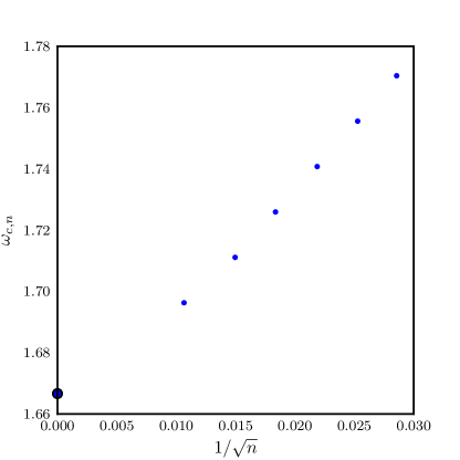
Figure 6: The peak position of the specific heat $\omega_{c,n}$ versus $1/\sqrt{n}$ for eISAT with $k=k_{G}$. The location of the kinetic growth point at $\omega=5/3$ is marked with a large dot on the vertical axis. One can see that the peak position of the specific heat approaches this point in the thermodynamic limit.

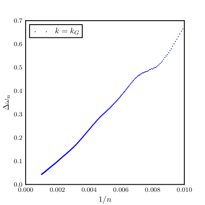
Figure 7: The half width the specific heat $\Delta\omega_{n}$ versus $1/n$ for eISAT with $k=k_{G}$.

Fig. 6 indicates that the peak position of the specific heat converges to the kinetic growth point $\omega_{c}=5/3$ with an expected inverse square-root like scaling, while Fig. 7 shows that the width of the transition decreases much faster with an inverse linear scale.

We thus conclude that

$$\omega_{c,n}-\omega_{c}\sim D\,n^{-1/2}\;,$$ (47)

where $\omega_{c,n}$ is the location of the peak of the specific heat, and

$$\Delta\omega_{n}\sim E\,n^{-1}\;,$$ (48)

where $\Delta\omega_{n}$ is the half-width (or, more precisely, width of the half-height) of the specific heat peak.

Since the width decays much faster than the shift, one cannot see the first-order nature of the true thermodynamic transition in a kinetic growth simulation which is fixed at the transition point; it lies outside the crossover region. This is graphically indicated in Fig. 8.

Figure 8: The observed scaling at $k=k_{G}$ is such that $(\omega_{c,n}-\omega_{c})\gg\Delta\omega_{n}$.

V.3 $k$-eISAT with $k>k_{G}$

We next discuss the case of $k>k_{G}$, where on the triangular lattice a first-order transition was found.

We simulated $k=5$, $k=7$, and a model where only triply visited sites are weighted (this can be seen as the limit of letting $k\to\infty$). We simulated trails with length up to $10^{3}$, collecting at that length $S_{n}\simeq 7\cdot 10^{8}$, $10^{9}$ and $2\cdot 10^{8}$ samples corresponding respectively to $S_{n}^{eff}\simeq 2\cdot 10^{7}$, $3\cdot 10^{7}$ and $4\cdot 10^{6}$ effective samples.

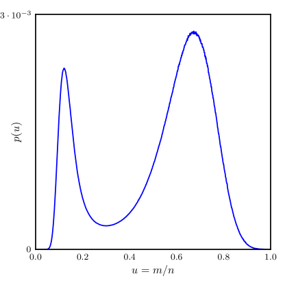
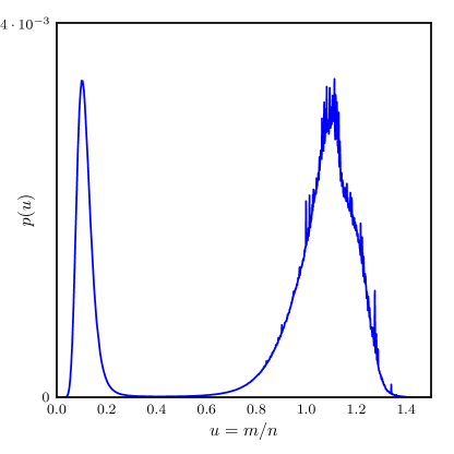
Figure 9: Normalised energy density of states ($k>k_{G}$) for $k=5$ and $7$, at the respective values of $\omega=1.65$ and $1.44$, i.e. near the peak of the specific heat curves.

The energy distribution displays a clear double peaked form (Fig. 9) which becomes more pronounced as $k$ increases. Moreover, it sharpens as $n$ increases, which is clear evidence of a first-order phase transition. We find that due to the initial build-up of the bi-modality the specific heat actually seems to increase faster than linearly. The scaling of the shift and width of the transition here is no longer consistent with the scenario found at $k=k_{G}$. We now find evidence for $1/n$ scaling of the shift of the transition, rather than the $1/\sqrt{n}$ scaling found at $k=k_{G}$.

V.4 $k$-eISAT with $k<k_{G}$

Finally we focus on $k$-eISAT for $k<k_{G}$. We simulated the $k$-eISAT model with $k=0,1,2,3$, collecting for each simulation order of $S_{n}\simeq 10^{8}$ samples (corresponding to $S_{e}^{eff}\simeq 10^{6}$) at the maximum length $N=10^{3}$.

On the triangular lattice, for $k<k_{G}$ the collapse transition is $\theta$-like, and hence second order. A corresponding conjecture for the cubic lattice is the presence of a weak second-order transition with a logarithmically divergent specific heat $c_{n}\simeq(\ln\,n)^{\zeta}$.

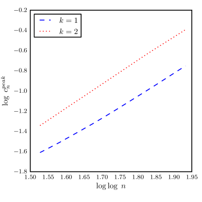
Figure 10: Specific heat peak scaling for $k=1$ and $k=2$: the specific heat diverges logarithmically with an exponent close to $\zeta=2.25$.

The results for $k=1$ and $k=2$, which we report in Fig. 10, are consistent with this prediction. However, we note that our estimated value $\zeta=2.25\pm 0.25$ is outside the prediction $\zeta=3/11$ for the $\theta$-point.

While models with $k=0$ and $k=3$ show very strong scaling corrections which make the analysis inconclusive there, we expect the second-order phase transition scenario to extend to these values, and indeed to the whole range of values $0\leq k<k_{G}$.

V.5 Low temperatures

Motivated by the results on the triangular lattice, we now investigate the possible presence of a crystal-like phase in three dimensions.

Figure 11: $1-3u_{3}$, the proportion of steps not involved with triply-visited sites per unit length, plotted against $n^{-2/3}$, for $(\omega_{2},\omega_{3})=(4,4)$ and $(\sqrt[7]{30},30)$, respectively.

In a crystal-like phase, in which the trail asymptotically fills the lattice, the quantity $1-3u_{3}$, i.e. the proportion of steps that are not involved with triply-visited sites per unit length, should tend to zero as $n\to\infty$. Based on this criterion, the investigation on the triangular lattice identified two different regions of the collapsed phase: one in which $1-3u_{3}$ tended to zero, and one in which it did not. The one in which it did was associated with the first-order transition for $k>k_{G}$.

Following the analysis in Doukas et al. (2010), we show in Fig. 11 the quantity $1-3u_{3}$ against $n^{-2/3}$ at two points in the parameter region of the low-temperature phase. This is the expected order of finite-size correction due to the presence of a surface in a compact low-temperature cluster. The parameters $(\omega_{2},\omega_{3})$ chosen are representative of regions in the $\omega_{2},\omega_{3}$–plane for which we would expect to observe a significant difference. While there is a substantial difference in the asymptotic value of $1-3u_{3}$ in these regions, it is clear that $1-3u_{3}$ does not tend to zero in either.

We have also looked for a signature of a transition between low temperature phases and were unable to find any emerging transition, unlike for the triangular lattice (see Fig. 13 below). Of course we cannot exclude that such a transition may become apparent at longer trail lengths.

VI Phase diagram

To investigate further the full two-dimensional phase diagram, we ran two more sets of simulations. First we ran a two-parameter flatPERM simulation of the general eISAT model. A simulation of this type is limited by both time and memory requirement but we have been able to collect $S_{n}^{eff}\simeq 10^{8}$ effective samples at length $N=512$.

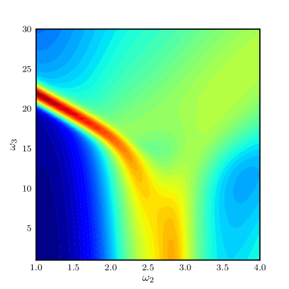
Figure 12: Density plot of the logarithm of the largest eigenvalue $\lambda_{max}$ of the matrix of second derivatives of the free energy with respect to $\omega_{2}$ and $\omega_{3}$ at length $n=512$.

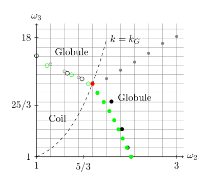
Figure 13: Schematic of the observed phase diagram at length $n=1000$. Dots indicate the location of peaks of fluctuations. Empty and filled dots indicate putative first and second order phase transitions, respectively, whereas small grey dots indicate crossover. The dot on the $k=k-G$-curve corresponds to the special transition described in Sec. V.1.

A density plot of the maximum fluctuations, calculated from the eigenvalues of the matrix of second derivatives of the free energy is shown in Fig. 12. Our inference for the finite size phase diagram is shown in Fig. 13.

Then we investigated the phase diagram along vertical and horizontal slices, that is to say with $\omega_{2}$ and $\omega_{3}$ fixed, for $n$ up to 1000. Observed phase transition points are included in Fig. 13. In the collapsed region we find evidence for a wide crossover region, but no evidence for an actual transition between two distinct phases.

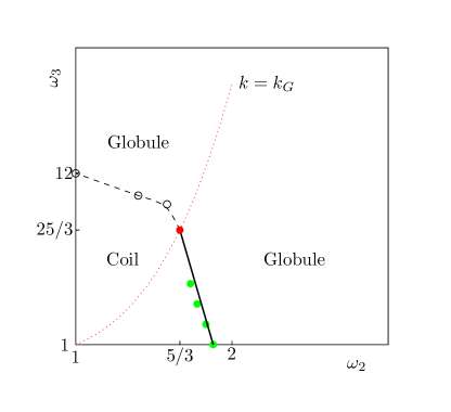
Figure 14: Conjectured phase diagram for cubic lattice. Solid lines indicate phase transitions of the second order while the dashed indicates a first-order phase transition. The red dotted line only indicates the $k$-eISAT model which passes through the KGT point. Empty and filled dots indicate an estimated location of the phase transitions coloured as in Fig. 13.

We have provided numerical evidence of that the two different types of transitions lead to a single collapsed globule-like phase at low temperatures. Our conjecture for the thermodynamic phase diagram is found in Fig. 14.

VII Conclusions

We have investigated the collapse properties of an extended family of interacting self-avoiding trails in three dimensions on the simple cubic lattice where doubly and triply visited sites are given weights $\omega_{2}=e^{\varepsilon_{2}/T}$ and $\omega_{3}=e^{\varepsilon_{3}/T}$.

We have explored the general eISAT model by considering a family of models satisfying $\omega_{3}=\omega_{2}^{k}$ with $k$ positive real number. A kinetic growth process (KGT) of growing trails on the cubic lattice maps to one temperature of the $k_{G}\simeq 4.15$ equilibrium model. We find that the collapse is second-order if $k<k_{G}$ and first-order if $k>k_{G}$. This resembles the triangular lattice finding (although the nature of the second order transition is different). Interestingly, the low temperature phase for both $k<k_{G}$ and $k>k_{G}$ seems to be a disordered globular state.

Exactly at $k=k_{G}$, the finite size scaling picture is particularly intriguing: the energy distribution displays a double peak form, indicating a first order type transition but we observe different values for the shift exponent $\psi\simeq 1/2$ and the width (crossover) exponent $\phi\simeq 1$. The thermodynamic limit location of this first order transition when $k=k_{G}$ is the temperature $T_{G}$ that maps to the kinetic growth process. However, if one simulates directly at the point $k=k_{G}$ and $T=T_{G}$ then the finite size scaling encountered is entirely second-order like and shows no sign of the first-order transition which dominates in the thermodynamic limit. This can be understood by appreciating that the finite size transition region shrinks quicker than its centre approaches the limiting temperature.

These results help to illuminate previous contradictory work for interacting trails on the diamond lattice Prellberg and Owczarek (1995); Grassberger and Hegger (1996). As the coordination number of the diamond lattice equals 4, trails can only interact through doubly visited sites. The collapse point of interacting trails on the diamond lattice at $\omega=3$ was identified with the kinetic growth process. In Prellberg and Owczarek (1995) it was shown that the scaling of the specific heat at the kinetic growth points for the diamond and simple cubic lattices was indistinguishable. However, simulations of interacting trails on the diamond lattice showed the emergence of a first-order phase transition Grassberger and Hegger (1996). The scenario we describe here for KGT on the simple cubic lattice clearly mimics these results. We are now able to understand the existence of both of these behaviours through the breaking of crossover scaling.

One last observation we can make is that interacting trails have been simulated in high dimensions Prellberg and Owczarek (2001); Owczarek and Prellberg (2003) and also demonstrate the breakdown of crossover scaling. The behaviour in high dimensions has been shown to be consistent with a self-consistent mean-field theory, which also displays bimodal energy distributions, though these do not lead to real first-order transitions in high dimensions. While that theory cannot not be applicable to $k=k_{G}$ in three dimensions (it predicts shift and width exponents both equal to $1/2$), it would be interesting to formulate a mean-field theory of the transition that occurs for our eISAT model when $k=k_{G}$. Consequently this may imply that the upper critical dimension for the $k=k_{G}$ eISAT models is less than three, and may in fact be two. Here we point out the numerical observation of confluent logarithms in the two-dimensional kinetic growth trails Owczarek and Prellberg (1995, 2006), lending further support to that assertion as logarithmic corrections typically appear at the upper critical dimension of a phase transition.

VIII acknowledgment

Financial support from the Australian Research Council via its support for the Centre of Excellence for Mathematics and Statistics of Complex Systems is gratefully acknowledged by the authors. The simulations were performed on the computational resources of the Victorian Partnership for Advanced Computing. A.L.O. thanks the School of Mathematical Sciences, Queen Mary University of London for hospitality.

References

- de Gennes (1975) P.-G. de Gennes, J. Physique Lett. 36, L55 (1975).
- Stephen (1975) M. J. Stephen, Phys. Lett. A. 53, 363 (1975).
- Duplantier (1982) B. Duplantier, J. Physique 43, 991 (1982).
- Duplantier (1986) B. Duplantier, Europhys. Lett. 1, 491 (1986).
- Duplantier (1987) B. Duplantier, J. Chem. Phys. 86, 4233 (1987).
- Meirovitch and Lim (1990) H. Meirovitch and H. A. Lim, J. Chem. Phys. 92, 5155 (1990).
- Prellberg (2001) T. Prellberg, J. Phys. A 34, L599 (2001).
- Prellberg and Owczarek (2001) T. Prellberg and A. L. Owczarek, Physica A 297, 275 (2001).
- Shapir and Oono (1984) Y. Shapir and Y. Oono, J. Phys. A. 17, L39 (1984).
- Lim et al. (1988) H. A. Lim, A. Guha, and Y. Shapir, J. Phys. A 21, 773 (1988).
- Owczarek and Prellberg (1995) A. L. Owczarek and T. Prellberg, J. Stat. Phys. 79, 951 (1995).
- Prellberg and Owczarek (1995) T. Prellberg and A. L. Owczarek, Phys. Rev. E. 51, 2142 (1995).
- Owczarek and Prellberg (2006) A. L. Owczarek and T. Prellberg, Physica A 373, 433 (2006).
- Doukas et al. (2010) J. Doukas, A. L. Owczarek, and T.Prellberg, Phys. Rev. E 82, 031103 (12pp) (2010).
- Clisby et al. (2007) N. Clisby, R. Liang, and G. Slade, J. Phys. A. 40, 10973 (2007).
- Owczarek et al. (1993) A. L. Owczarek, T. Prellberg, and R. Brak, Phys. Rev. Lett. 71, 4275 (1993).
- Brak et al. (1993) R. Brak, A. L. Owczarek, and T. Prellberg, J. Phys. A. 26, 4565 (1993).
- Lawrie and Sarbach (1984) I. D. Lawrie and S. Sarbach, in Phase Transitions and Critical Phenomena, edited by C. Domb and J. L. Lebowitz (Academic, London, 1984), vol. 9.
- Prellberg and Owczarek (2002) T. Prellberg and A. L. Owczarek, Comp. Phys. Commun. 147, 629 (2002).
- Lyklema (1985) J. Lyklema, J. Phys. A. 18, L617 (1985).
- Prellberg and Krawczyk (2004) T. Prellberg and J. Krawczyk, Phys. Rev. Lett. 92, 120602 (2004).
- Janse van Rensburg (2009) E. J. Janse van Rensburg, J. Phys. A 42, 323001 (2009).
- Grassberger and Hegger (1996) P. Grassberger and R. Hegger, J. Phys. A. 29, 279 (1996).
- Owczarek and Prellberg (2003) A. L. Owczarek and T. Prellberg, Int. J. Mod. Phys. C. 14, 621 (2003).