Universality in Bibliometrics

Abstract

Many discussions have enlarged the literature in Bibliometrics since the Hirsh proposal, the so called $h$-index. Ranking papers according to their citations, this index quantifies a researcher only by its greatest possible number of papers that are cited at least $h$ times. A closed formula for $h$-index distribution that can be applied for distinct databases is not yet known. In fact, to obtain such distribution, the knowledge of citation distribution of the authors and its specificities are required. Instead of dealing with researchers randomly chosen, here we address different groups based on distinct databases. The first group is composed by physicists and biologists, with data extracted from Institute of Scientific Information (ISI). The second group composed by computer scientists, which data were extracted from Google-Scholar system. In this paper, we obtain a general formula for the $h$-index probability density function (pdf) for groups of authors by using generalized exponentials in the context of escort probability. Our analysis includes the use of several statistical methods to estimate the necessary parameters. Also an exhaustive comparison among the possible candidate distributions are used to describe the way the citations are distributed among authors. The $h$-index pdf should be used to classify groups of researchers from a quantitative point of view, which is meaningfully interesting to eliminate obscure qualitative methods.

, , and

1 Introduction

The scientific community has not been the same after the publication of the polemic index of Hirsh ($h$-index). If an author has $h$-index equal to $h$ means that she has $h$ papers with at least $h$ citations but she has not $h+1$ papers with at least $h+1$ citations [1]. This definition leads to an important fact: an author with index $h$ has at least $h^{2}$ citations [1], a lower bound in the citation number.

This simple but powerfull idea has also suscitated other informetric formulations [2]. This index joins attributes as: productivity, quality and homogeneity in the same measure. It has also been used as one of the most important measures to quantify scientists in order to obtain fairer rankings [3]. Fairer rankings should mean, for example, grants fairer distributed among scientists really based on capability therefore it must stimulate a healthy competition.

Other successful variations of the $h$-index have been proposed. For instance, dividing the $h$ top papers index by the average of authors in these $h$ papers leads to: $h_{I}=h^{2}/N_{t}$ [4]. Considering that a massive part of publications cannot be used to compute the $h$-index, an interesting and alternative index that considers the weight of this mass of these lazy papers has been proposed in Refs [5, 6, 7]). Other metrics consider that not an individual $h$-index for each scientist might be considered but also its version for a group of researchers, which is denoted as successive $h$-index [8, 9].

Laeherre and Sornette [10] were the first to address the researcher citation distribution. They have ranked 1120 physicists according to their total number of citations. The number of researchers $N(x)$ as function of their citation number $x$ follows a stretched exponential function:

$$N(x)=N_{0}\exp[-(x/x_{0})^{\beta}]$$ (1)

with $\beta\approx 0.3$. Here $N_{0}=N(0)$ is number of authors with no citation and $x_{0}$ an parameter that can be estimated for example if the citation mean is known. Of course, citation number $x$ in an integer variable, but here we have considered it as a continuous variable.

Alternatively, Redner [11] has also addressed this questioning in a slightly different way. The probability distribution of citations of 783.339 scientific papers, not authors, published in 1981, with the 6.716.198 citations obtained between 1981 and 1997 in the base Institute of Scientific Information (ISI) has been studied. The envelope of this distribution presents a stretched exponential behavior for low citation number $x<x_{c}$, with $x_{c}=200$ and for large citation number $x>x_{c}$, the power law behavior is dominant $N(x)\sim x^{-\alpha}$, with $\alpha\approx 3.0$.

Tsallis and Albuquerque [12] observed that Redner’s probability distribution function (pdf) and the paper (not author) citation pdf could be better described by a generalized exponential distribution that covered the two situations ($x\leq x_{c}$ and $x>x_{c}$):

$$N_{q}(x)=N_{0}[\exp_{q}(-\lambda x)]^{q}$$ (2)

where generalized exponential function ($q$-exponential) is $\exp_{q}(x)=[1+(1-q)x]^{1/(1-q)}$, if $(1-q)x\geq-1$ and it vanishes otherwise. The $q$-exponential inverse function is the $q$-logarithm: $\ln_{q}(x)=(x^{1-q}-1)/(1-q)$ [13, 14, 15]). The parameter $\lambda$ in Eq. (2) is obtained constraining the citation per paper average number to be a constant, $\left\langle x\right\rangle=\int_{0}^{\infty}dx\ x\ P_{q}(x)=$ constant, where $P_{q}(x)=[\exp_{q}(-\lambda x)]^{q}/\int_{0}^{\infty}dy[\exp_{q}(-\lambda y)]^{q}$. Although in Ref. [12], this approach has been used only for distribution of scientific papers, we show that it can be also applied for author citation probability distribution.

Here, we consider the stretched and generalized exponential pdf’s to describe the envelope of the author citation distribution. Also, we ask which pdf is more appropriate to describe the $h$-index distribution of authors of distinct groups of researchers. Using a continuous approximation for citation distributions, two different researcher groups are collected from two different database. One from Graduate Programs in Physics and Biology of public universities in Brazil using their ISI publication registry. The other, from software engineering area, where we computed the $h$-indices and the total citations of the members of program committees of different conferences. It is important to stress, that our purpose, is to show that the same $h$-index pdf is verified even in “soft” databases more suitable to areas that are not based strictly on journal publications. If different models follow the same law, in statistical physics, one says that this law is universal, in fact there are classes of universality. We question, if the two mentioned groups of authors, of different areas with data collected from different databases, have the same pdf, and which one is better to describe the data.

This paper is organized as follows. In Sec. 2, we show the details of deduction of the generalized distribution of $h$-indices extracted from different citation distributions for different approaches: i) The first one establishes that citation distribution follows a escort probability distribution according to Eq. (2); ii) The other one prescribes that citations are distributed according to a stretched exponential via equation (1). In Sec. 3 we present the details about databases used to test h-index distribution formula. We describe with some details how the data were extracted for each studied group. In Sec. 4, we present our results, which can be separated in two distinct parts. In a first (preliminary) part we estimate necessary parameters of the citation distributions i) and ii) previously reported by using the method of moments and by comparisons of the theoretical and empirical cumulated citation distribution. Secondly, we so obtain the $h$-index distribution by studying it for the distinct areas. The parameters obtained from $h$-index distribution fits are compared with the same parameters estimated by citation distribution fits and we conclude that generalized statistics produce a $h$-index distribution that corroborates the citation distribution differently from stretched exponential that points out more accentuated differences between these two ways of estimation. We finally summarize our results as well as highlight our main contributions in Sec. 5.

2 $h$-index probability density functions for groups of authors

In this section, we consider the continuous limit of normalized citation distribution and we describe a deduction of the distribution of $h$-indices for a group of authors for the stretched [10] and generalized [12] exponential pdf’s, which are confronted next section.

The fundamental Hirsch hypothesis [1] leads to $x=ch^{2}$, where $c$ is a constant, which is determined making a suitable linear fit. Since the databases supplies the number of citations ($x_{i}$) and the corresponding $h$-index of the $i^{\mbox{th}}$ author ($h_{i}$), with $i=1,\ldots,n$, one has an estimator to mean citation number $\langle x\rangle$ and $c$. Collecting a sample of citations of all authors of a group, which we denote by $x_{1},x_{2},\ldots,x_{n}$ corresponding to the respective $n$ authors, the estimate of $\left\langle x\right\rangle$, denoted by $\widehat{x}$, is the simple arithmetic mean:

$$\widehat{x}=\frac{x_{1}+x_{2}+...+x_{n}}{n}\;.$$ (3)

Similarly, an estimator $\widehat{c}$ for the coefficient $c$ comes from least square fitting:

$$\widehat{c}=\frac{\sum\limits_{i=1}^{n}h_{i}^{2}x_{i}-\dfrac{1}{n}\sum\limits_{i=1}^{n}h_{i}^{2}\sum\limits_{j=1}^{n}x_{j}}{\sum\limits_{i=1}^{n}h_{i}^{4}-\dfrac{1}{n}\left(\sum\limits_{i=1}^{n}h_{i}^{2}\right)^{2}}\;,$$ (4)

that measures the slope in the linear fit of the plot $x$ versus $h^{2}$.

2.1 Stretched Exponential PDF

One interesting pdf used to study the citation distribution is the stretched exponential pdf tha we define in the continuous case as:

$$P_{\beta}(x)=\frac{\beta}{x_{0}\Gamma(1/\beta)}\;e^{-(x/x_{0})^{\beta}}\;.$$ (5)

One can estimate $x_{0}$ by calculating $\left\langle x\right\rangle$, which, in turn, is estimated by $\widehat{x}$, i.e., we can demand the condition $\left\langle x\right\rangle=\int\limits_{0}^{\infty}dxxP_{\beta}(x)=x_{0}\Gamma(2/\beta)/\Gamma(1/\beta)=\widehat{x}$, resulting in:

$$\widehat{x}_{0}\approx\frac{\Gamma(1/\beta)}{\Gamma(2/\beta)}\;\widehat{x}\;.$$ (6)

According to $x=ch^{2}$, the $h$-index pdf for the stretched exponential is:

$$H_{\beta}(h)=\frac{2\widehat{c}\beta\Gamma(2/\beta)}{\widehat{x}\Gamma(1/\beta)^{2}}\;h\;\exp\left[-\left(\frac{\widehat{c}\;\Gamma(2/\beta)h^{2}}{\Gamma(1/\beta)\widehat{x}}\right)^{\beta}\right]\;.$$ (7)

In section 4 we will show fits of the $h$-index histograms for the distinct analyzed groups using this pdf. Now let us obtain another formula for $h$-index pdf by using the proposal of generalized exponentials.

2.2 Generalized Exponential PDF

The generalized exponential approach, considers:

$$P_{q}(x)=\frac{[\exp_{q}(-\lambda x)]^{q}}{\int_{0}^{\infty}dy[\exp_{q}(-\lambda y)]^{q}}\;,$$ (8)

for $0<x<\infty$. To estimate $\lambda$, one analytically calculates the first moment of this pdf $\left\langle x\right\rangle=\int_{0}^{\infty}xP_{q}(x)dx=1/[(2-q)\lambda]$, with does not diverge for $1<q<2$. Next, one estimates $\lambda$ through

$$\widehat{\lambda}\approx\frac{1}{(2-q)\widehat{x}}$$ (9)

and a hybrid expression for the citation pdf, considering that $\widehat{x}$ is an estimator for $\left\langle x\right\rangle$ is:

$$\widehat{P}_{q}(x)=\frac{1}{(2-q)\widehat{x}}\;[\exp_{q}\{-x/[(2-q)\widehat{x}]\}]^{q}\;.$$ (10)

Now we are able to compute the $h$-index distribution for a group of researchers:

$$\begin{array}[]{lll}H_{q}(h)&=&\left|\frac{dx}{dh}\right|\;\widehat{\lambda}\;[\exp_{q}(-\widehat{\lambda}\widehat{c}h^{2})]^{q}\\ &&\\ &=&\dfrac{2\widehat{c}}{(2-q)\widehat{x}}\ h\ [\exp_{q}\left\{-\frac{\widehat{c}h^{2}}{(2-q)\widehat{x}}\right\}]^{q}\;,\end{array}$$ (11)

which is normalized. Since the parameters $\left\langle x\right\rangle$ and $c$ are estimated by $\widehat{x}$ and $\widehat{c}$, respectively, the only free parameter is $q$.

Now we have two candidates for $h$-index pdf. These pdf’s are used to fit our data for the two different groups of researchers.

3 Databases

Two different researcher groups are collected from two different databases. The first database is obtained from 1203 researchers from 19 Graduate Programs in Physics (600 researchers) and 26 Graduate Programs in Biology (603 researchers) of public universities in Brazil. To obtain the published papers, we have used the data from the research digital curriculum vitae at public disposal at the Lattes database (http://lattes.cnpq.br/english), which is a well-established and conceptualized database [16], where most Brazilian researchers deposit their vitae. By a manual process, each researcher publication has been extracted from this platform and compared to the ISI-JCR database by crossing the information between these two bases.

It is important to notice that refinements on queries were performed for suitably computing the $h$-index of author. We tune the details of query performed on ISI-JCR until number of papers of queried author in this database is the same or as close as possible of that one registered by author in its Lattes vitae. Only after this process, we compute the authors $h$-index.

The same process is run out for each researcher of the studied group. This method, although manual is an excellent filter to obtain data for Brazilian researchers.

In many areas as Computer Science, the authors are ranked considering not only papers published in scientific journals, but also by papers published in important conferences. For sake of the simplicity, we concentrate our analysis in software engineering area by computing the $h$-indices and the total citations of the members of program committees of seven different conferences in a total of 600 researchers. For these authors, we have used the Harzing program, that computes the $h$-index based on google-scholar index. The choice to use Google Scholar instead of ISI-JCR for computer scientists is because many important conferences are not captured by ISI-JCR database. It is important to stress, that our intention, is to show that the universality of $h$-index pdf is verified even in “soft” databases more suitable to areas that are not based strictly on journal publications. Also, the number of considered researchers in Harzing has not been greater because there is a blockage of the system after a number of searches, which make our job much more vagarious.

4 Results

Our main results are presented below. Consider the researchers from Post-Graduations in Physics and Biology as Group I and from Conferences Computer Science (Harzing/Google Scholar) as Group II. The plots of citation number as a function of each author $h^{2}$ are depicted in Fig. 1. The plots in Fig. 1 exhibit the behavior of the citation number as a function of $h^{2}$, for different authors in each one of the studied groups. The proportionality parameter $c$, given by Eq. 4, is numerically estimated. Plot (a) corresponds to data from Group I ($c=3.75(4)$) and Plot (b) is a similar plot for the Group II ($c=5.44(9)$). These $\widehat{c}$ estimates reflect the difference between the two areas.

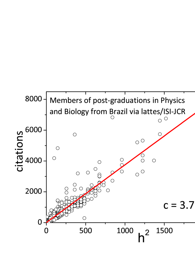
(a)

(b)

Figure 1: These figures exhibit the number of citations as function of $h^{2}$ of different authors, for different groups, used to estimate $c$ of Hirsch’s relation numerically obtained by 4. Plot (a), for members of post-graduate programs from Brazil obtained via Lattes platform-ISI-JCR. Plot (b), corresponds to data from members of committee programs of computer science conferences obtained by google-Harzing.

In what follows, we compute the parameters of citation pdf’s of both considered groups. The parameters of the stretched exponential pdf [10] and the generalized exponential pdf [12] are estimated using the method of moments.

4.1 Stretched Exponential PDF

For accurately estimating $\beta$ in Eq. (5), we firstly use the method of moments and compare it with the value obtained from the Zipf plot. The method of moments consists in calculating the $k^{\mbox{th}}$ moment of the pdf comparing them with the experimental ones. Consider the moments of the stretched exponential pdf:

$$\left\langle x^{k}\right\rangle=\frac{\beta}{x_{0}\Gamma(1/\beta)}\;\int_{0}^{\infty}dxx^{k}\;e^{-(x/x_{0})^{\beta}}=\frac{x_{0}^{k}}{\Gamma(1/\beta)}\Gamma(\frac{k+1}{\beta})\;.$$

The experimental moments are calculated as $\overline{x^{k}}=(x_{1}^{k}+x_{2}^{k}+...+x_{n}^{k})/n$. The method consists in calculating the best $\beta$ value that matches both numerically calculated $\left\langle x^{k}\right\rangle$ and $\overline{x^{k}}$ for several $k$ values (not only for integers). Since $\left\langle x^{k}\right\rangle$ depends on $x_{0}$, one considers the ratio

$$\Phi_{k}^{(\beta)}=\frac{\langle x^{k}\rangle}{\langle x\rangle^{k}}=\frac{\Gamma^{k-1}(1/\beta)\Gamma[(k+1)/\beta]}{\Gamma^{k}(2/\beta)}$$ (12)

to eliminate the $x_{0}$ dependence. The corresponding experimental ratio

$$\Phi_{k}^{(\exp)}=\frac{\overline{x^{k}}}{\overline{x}^{k}}=\frac{\sum\nolimits_{i=1}^{n}x_{i}^{k}}{(\sum_{i=1}^{n}x_{i})^{k}}\;.$$ (13)

Form the numerical minimization of $\int(\Phi_{k}^{(\beta)}-\Phi_{k}^{(\exp)})^{2}dk$, using $\delta k=0.01$, one obtains $\beta=0.47$ for Group I and $\beta=0.31$ for Group II. In Fig. 2, we show plots of theoretical moments for several $\beta$ values and the experimental moments in same plot for both groups studied here.

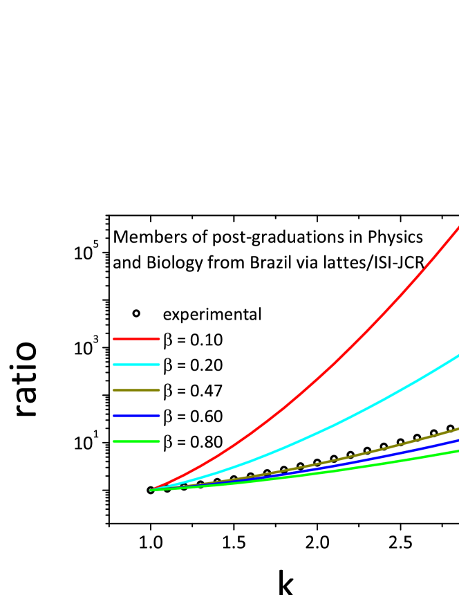
(a)

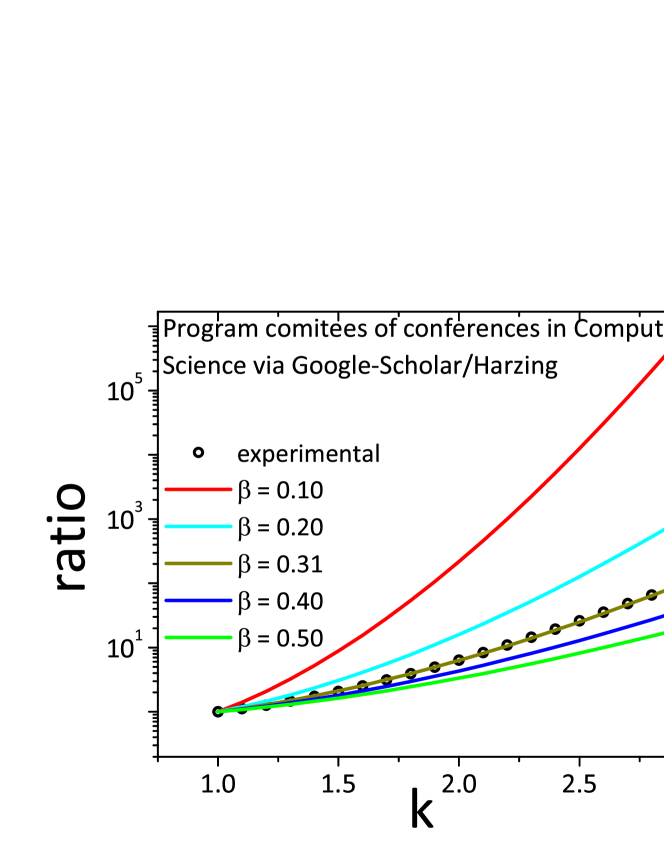
(b)

Figure 2: These plots exhibit the theoretical moments based on citations stretched exponential pdf (Eq. 12), compared with experimental moments (Eq. 13) for group I (a) with $\beta=0.47$ and II (b) with $\beta=0.31$.

The result for Group I, even for the same database (ISI-JCR), clearly is different from that found in Ref. [10]. However, the result for Group I is closer of exponent for the citations of papers (not of authors) from journal Physical Review D ($\beta\approx 0.39$) and similar to citations of the papers from ISI ($\beta\approx 0.44$) obtained in Ref. [11], in the limit of low citations ($x<500$). Although the value found for Group II corroborates the value found in Ref. [10] ($\beta\approx 0.3$), no matching was expected because this last result was obtained for citations of 1120 most cited authors obtained from ISI-JCR, during a time-lag (between 1981-1997) and our results are based on all citations of scientific life of considered authors.

To test the quality of our fits, we also considered suitable Zipf plots. The main idea of Zipf plot is to rank the citations of all authors according to $x_{1}\geq x_{2}\geq x_{3}...\geq x_{n}$. The upper tail distribution is expected to be:

$$\zeta_{j}=\int_{x_{j}}^{\infty}P_{\beta}(x)dx=1-\frac{j}{n}$$ (14)

where $j$ is the rank of citation $x_{j}$. For the stretched exponential, one has:

$$\zeta_{j}=\frac{\beta}{\widehat{x}}\frac{\Gamma(2/\beta)}{\Gamma(1/\beta)}\int_{x_{j}}^{\infty}dx\exp[\frac{-\Gamma(2/\beta)^{\beta}}{\Gamma(1/\beta)^{\beta}\overline{x}^{\beta}}x^{\beta}]=\frac{\Gamma(1/\beta,\frac{\Gamma(2/\beta)^{\beta}x_{j}^{\beta}}{\Gamma(1/\beta)^{\beta}\widehat{x}^{\beta}})}{\Gamma(1/\beta)}\;,$$ (15)

where $\Gamma(a,b)=\int_{b}^{\infty}z^{a-1}e^{-z}dz$ is known as the incomplete gamma function.

In Fig 3, we display the Zipf plots ($\zeta_{j}$ as function of $j/n$), using $\beta=0.47$ for Group I and $\beta=0.31$ for Group II. One can see a near linear behavior with slope close to $-1$ and intercept close to $1$, the expected values for both cases. However, some discrepancies are present. For sake of comparison, we show the linear fit (red continuous line) and an exact expected behavior (dashed blue line).

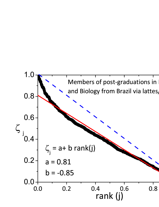
(a)

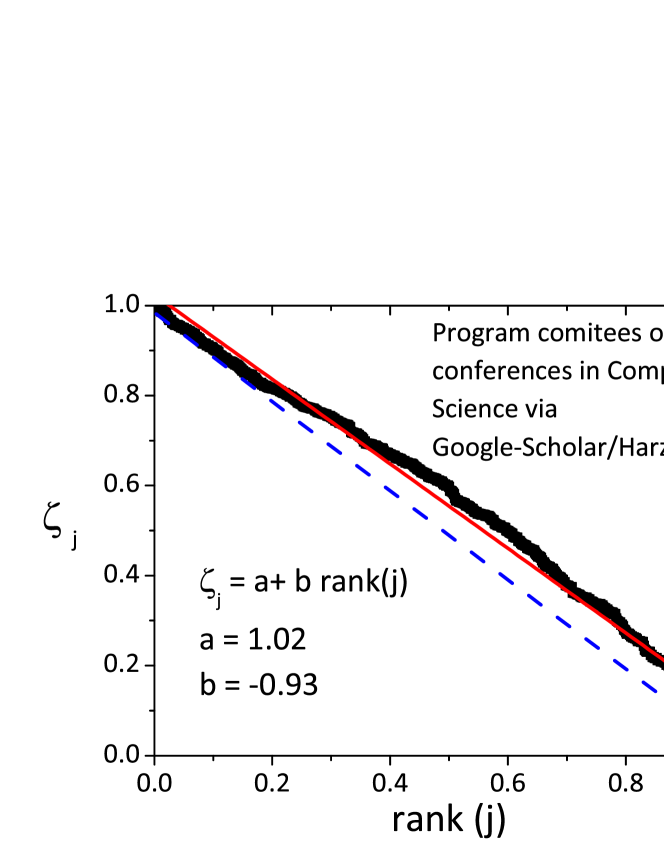
(b)

Figure 3: Zipf plots for the stretched exponential pdf for: (a) Group I and (b) Group II. The expected linear behavior by relation 14 is tested plotting $\zeta_{j}$ calculated by 15 as function of $j/n$.

4.2 Generalized Exponential PDF

Now we consider the generalized exponential pdf. The moment method is addressed using the ratio:

$$\Psi_{k}=\frac{\left\langle x^{k}\right\rangle_{q}}{\left\langle x\right\rangle_{q}^{k}}=\frac{1}{(2-q)\widehat{x}^{k+1}}\int_{0}^{\infty}dx\ x^{k}\left[1+\frac{(q-1)}{(2-q)\overline{x}}x\right]^{q/(1-q)}\;,$$ (16)

where only the first moment $\left\langle x\right\rangle_{q}$ is estimated as simple averages: $\widehat{x}=473(23)$ for Group I and $\widehat{x}=936(76)$, for Group II. Similarly to the stretched exponential case, we use the same procedure: compare $\Psi_{k}$ with the experimental moments ($\Phi_{k}^{(\exp)}$) calculated by Eq. (13). These plots are displayed in Fig. 4 and the best adjusted values are $q=1.27$, for Group I and $q=1.37$, for Group II.

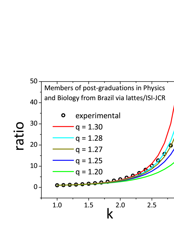
(a)

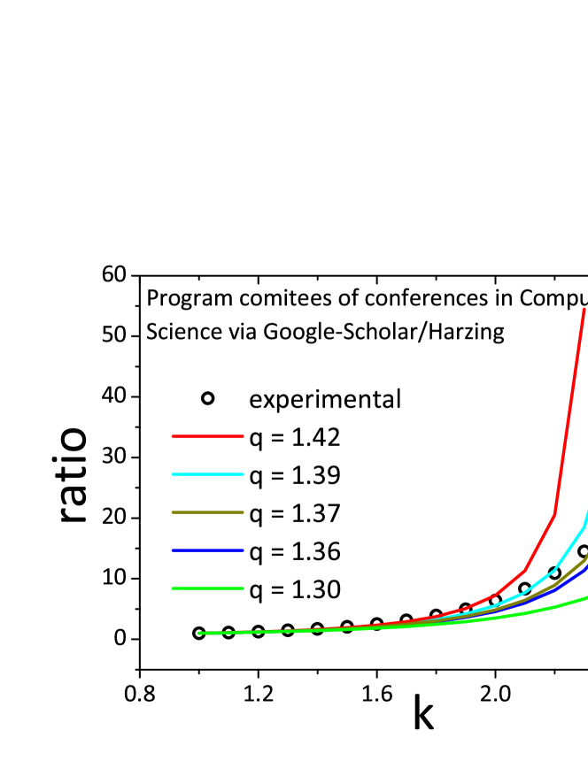
(b)

Figure 4: These plots exhibit the theoretical moments based on citations generalized exponential pdf (Eq. 16), compared with experimental moments (Eq. 13) for group I (a) with $q=1.27$ and II (b) with $q=1.37$.

The upper tail distribution for the generalized exponential is:

$$\begin{array}[]{lll}\zeta_{j}&=&\int_{x_{j}}^{\infty}P_{q}(x)dx\\ &&\\ &=&\frac{1}{(2-q)\overline{x}}\int_{1+\frac{(q-1)}{(2-q)\overline{x}}x_{j}}^{\infty}x^{q/(1-q)}dx\\ &&\\ &=&\exp_{q}\left(\frac{-x_{j}}{(2-q)\overline{x}}\right)\end{array}\;.$$

Similarly to Fig. 3, we have used the values of $\widehat{x}$ to plot $\zeta_{j}$ as function of rank ($j/n$) as illustrated in Fig. 5.

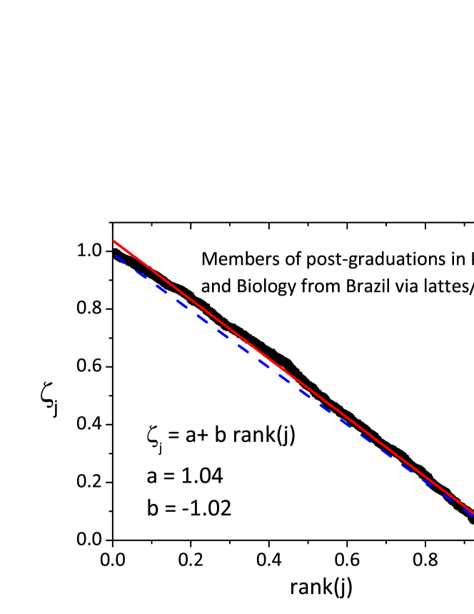
(a)

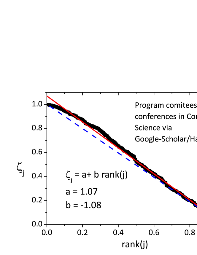
(b)

Figure 5: Zipf plots for the stretched exponential pdf for: (a) Group I and (b) Group II.

From Figs.  3 and 5, one observes a better linear fit for the Zipf plots using the generalized exponential pdf. However an important question is if the same values of $q$ here estimated for citation distribution are also estimated when we perform $h$-index distribution fits.

4.3 $h$ index PDF

In Table 1, we summarize the estimated parameters for the stretched and generalized exponential pdf’s using the method of moments and Zipf plots.

Groups	$c$	$\widehat{c}$	$\beta$	$\widehat{x}$	$q$
I	3.75(4)	$3.77(5)$	0.47(1)	473(23)	1.27(1)
II	5.44(9)	$5.71(11)$	0.31(1)	936(76)	1.37(1)

Table 1: Summary of the parameter estimated by the method of moments for the citation distribution pdf which was fitted as stretched exponential and as generalized exponential. Group I refers Researchers from Post-Graduations in Physics and Biology (Lattes/CNPq-ISI-JCR). Group II refers Conferences Computer Science (Harzing/Google Scholar). The coefficient $c$ is obtained by fits of the plots of Fig. 1. The coefficient estimator $\widehat{c}$ is calculated from Eq. 4. The stretched exponential parameter $\beta$ is obtained by the best matching via method of moments shown in Fig. 2. The average estimator $\widehat{x}$ is the simple arithmetic mean. The generalized exponential parameter $q$ is similarly obtained according to Fig. 4.

Let us now consider the databases $h$-indices pdfs compared to the stretched and generalized exponential pdf’s [Eqs. (7) and (11)]. Using the estimates of $\widehat{c}$ and $\widehat{x}$ for each group studied (see table 1), we find numerically the $\beta$ that minimizes $\chi_{\beta}^{2}=\sum_{h=h\min}^{h_{\max}}\left[f^{(\exp)}(h)-H_{\beta}(h)\right]^{2}$ for the stretched exponential pdf and $q$ that minimizes $\chi_{q}^{2}=\sum_{h=h\min}^{h_{\max}}\left[f^{(\exp)}(h)-H_{q}(h)\right]^{2}$ for the generalized exponential pdf, where $H_{\beta}(h)$ is computed by Eq (7) and $H_{q}(h)$ by Eq. (11). Our computer code runs with $q$ ranging from $q_{\min}=1.01$ up to a $q_{\max}=1.99$ and $\beta$, from $\beta_{\min}=0.01$ up to a $\beta_{\max}$ $=0.99$ in steps of $\Delta q=\Delta\beta=0.01$. The best fits, according to the $\chi^{2}$ measures, give $\beta=0.66(1)$ and $q=1.26(1)$, for Group I and $\beta=0.64(1)$ and $q=1.24(1)$, for Group II using the stretched and generalized exponential pdf’s, respectively. Both pdf’s are depicted in Fig. 6 and the comparison among the estimated parameters to the ones of Table 1, is compiled in Table 2.

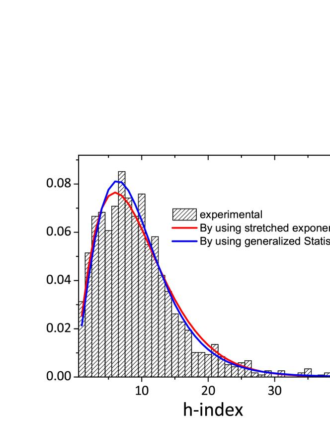
(a)

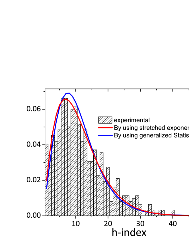
(b)

Figure 6: $h$-index distribution for (a) Group I and (b) Group II. Blue line corresponds to the stretched exponential pdf (Eq. 7) and the red line to the generalized exponential pdf (Eq. 11).

Groups	$\beta_{m}$	$\beta_{\chi^{2}}$	$q_{m}$	$q_{\chi^{2}}$
I	0.47(1)	0.66(1)	1.27(1)	1.26(1)
II	0.31(1)	0.64(1)	1.37(1)	1.24(1)

Table 2: Comparison of the stretched and generalized exponential pdf’s parameters estimated by the method of moments and $\chi^{2}$ procedures. One sees that the generalized exponential pdf, has a more robust estimation that the stretched exponential pdf.

Although, from Fig. 6, one can see good fits for both pdf’s, from Table 2, one observes that generalized exponential pdf produces a much better matching among the estimated parameter, via citation distribution through the moment method and $h$-index distribution through the $\chi^{2}$ method than the stretched exponential pdf. For Group I, for the generalized exponential pdf, we have an exact estimated parameter showing its greater robustness when compared to the stretched exponential pdf. It is important to notice that for Group II, both pdf’s produce more distant estimates.

Our results indicate that the generalized exponential pdf is more appropriate to describe the $h$-index pdf, supplying an interesting and simple formulae for $h$-indices of very distinct groups in different databases. Since the data have been collected from very different sources, one can claim the universal aspect of the generalized exponential pdf to represent the continuous $h$-index.

5 Conclusions

In the first part of this manuscript, we analyze the different formulas for citation distribution calculating their parameters via two different methods: method of moments and by Zipf plots for two very distinct groups of researchers pertaining to different databases. In the second part, we calculate the $h$-index distribution also for these different databases to find a universal formula. Our results show that good fits can be obtained for the $h$-index pdf using suitable estimates and the relation $x=ch^{2}$. It is also important to mention that we have estimated the parameters $\beta$ and $q$ in two independent ways and by moments and $\chi^{2}$ methods: the citation distribution of Eqs. (5) and (10) and $h$-index distribution of Eqs. (7) and (11). Such fits produce more similar results for the $q$ distributions.

References

- [1] J. E. Hirsch, An Index to quantify and individual´s scientific research output, PNAS, 102, 46, 16569-16572 (2005)
- [2] L. Egghe, R. Rosseau, An informetric model fo the Hirsch index, Scientometrics, 69, 1, 121-129 (2006)
- [3] Index aims for fair rankings of scientists, Nature 436, 900 (2000)
- [4] P. D. Batista, M. G. Campiteli, O. Kinouchi, A. S. Martinez, Is it possible to compare researchers with different scientific interests?. Scientometrics, 68, 1, 179-189 (2006)
- [5] L. Egghe, Theory and practise of the g-index, Scientometrics, 69, 1, 131–152(2006)
- [6] R. S. J. Tol A rational, successive g-index applied to economics departments in Ireland, Journal of Informetrics, 2, 149–155 (2008)
- [7] Woeginger, G.J. An axiomatic analysis of Egghe’s g-index, Journal of Informetrics, 2, 364–368 (2008)
- [8] L. Egghe, Modelling sucessive -indices, Scientometrics, 77, 3, 377-387 (2008)
- [9] A. Schubert, Successive -indices, Scientometrics, 70, 1, 201–205 (2007)
- [10] J. Laherrere, D. Sornette, Stretched exponential distributions in nature and economy: fat tails with characteristic scales, Eur. Phys. J, B2, 525-539 (1998)
- [11] S. Redner, How Popular is your paper? An Empirical Sudy of the Citation Distribution, Eur. Phys. J, B4, 131-134 (1998)
- [12] C. Tsallis, M. P. Albuquerque, Are citation of scientific papers a case of nonextensivity? Eur. Phys. J. B13, 777-780 (2000)
- [13] C. Tsallis, Nonextensive Statistics: Theoretical, Experimental and Computational Evidences and Connections, Brazilian Journal of Physics, 29, 1, 1-35 (1999)
- [14] C. Tsallis, Introduction to Nonextensive Statistical Mechanics – Approaching a Complex World, Springer (2009)
- [15] T. J. Arruda, R. S. González, C. A. S. Terçariol, A. S. Martinez, Arithmetical and geometrical means of generalized logarithmic and exponential functions: generalized sum and product operators, Phys. Lett. A 372 (2008) 2578–2582.
- [16] J. Lane, Let’s make science metrics more scientific, Nature, 464, 488-489 (2010)