section[6mm]6mm0pc *subsection[6mm] , [  •  ][]

TIFR/TH/11-46

arXiv:1111.2839v3

        Abstract

We study classical and quantum finite-size corrections to giant magnons in $AdS_{4}\times CP^{3}$ using generalised Lüscher formulae. Lüscher F-terms are organised in powers of the exponential suppression factor $(e^{-\Delta/2h})^{m}$, and we calculate all terms in this series, matching one-loop algebraic curve results from our previous paper [1]. Starting with the second term, the structure of these terms is different to those in $AdS_{5}\times S^{5}$ thanks to the appearance of heavy modes in the loop, which can here be interpreted as two-particle bound states in the mirror theory. By contrast, physical bound states can represent dyonic giant magnons, and we also calculate F-terms for these solutions. Lüscher $\mu$-terms, suppressed by $e^{-\Delta/E}$, instead give at leading order the classical finite-size correction. For the elementary dyonic giant magnon we recover the correction given by [2]. We then extend this to calculate the next term in $1/h$, giving a one-loop prediction. Finally we also calculate F-terms for the various composite giant magnons, $RP^{3}$ and ‘big’, again finding agreement to all orders.

Contents

toc

1 Introduction

The Lüscher formulae arise from one-loop Feynman diagrams in which a propagator circles the space [3, 4, 5]. Since such diagrams are the only ones not present in infinite volume, they give finite-volume corrections. And because the large-volume limit puts this propagator on-shell, they can be written in terms of the S-matrix for asymptotic states.

In the AdS/CFT context, the relevant spatial circle is either the position along the spin chain (at weak coupling) or else on the worldsheet of a closed string (at strong coupling), and the S-matrix is known for all values of the coupling [6, 7, 8, 9]. At weak coupling, Lüscher corrections can be successfully summed to reach all the way to the shortest nontrivial chain, the Konishi operator [10]. In this paper however we will be working on the string side of the correspondence, and following [11, 12, 13] to look at corrections to giant magnons [14]. These initially have $E=\Delta-J/2$ finite, with $\Delta$ infinite, and we will be interested in exponential corrections starting with these:

$$\delta E^{F}=\underset{\vphantom{1^{\frac{1}{1^{1}}^{1}}}\mbox{ first F-term }}{e^{-\Delta/2h}a_{1,0}}+\underset{\vphantom{1^{\frac{1}{1^{1}}^{1}}}\mbox{ second F-term }}{\big{(}e^{-\Delta/2h}\big{)}^{2}a_{2,0}}+\>\mathcal{O}\big{(}e^{-\Delta/2h}\big{)}^{3}.$$ (1)

We will calculate these for the correspondence between ABJM theory and IIA strings in $AdS_{4}\times CP^{3}$ [15, 16], using the all-loop S-matrix of [17]. (For the related asymptotic Bethe ansatz, see [18].) Lüscher corrections in this theory were also studied by [19, 20, 21, 22].

Our first goal is to compare these F-terms to the string theory calculation of [1]. There we computed semiclassical corrections to the energy of giant magnons, both in infinite volume, and obtaining a series of exponential corrections. The subtleties of that calculation arose from the presence of heavy modes, and how to impose a cutoff on these. The first F-term depends only on the light modes, but the second F-term also has a contribution from the heavy modes.

The existence of heavy and light modes is a novel feature of this version of the correspondence, compared to the more familiar SYM / $AdS_{5}\times S^{5}$ case. From the sigma-model perspective they are simply half the directions in target space, where some have radius of curvature $R$ and some $R/2$. (Although some interesting effects are seen at one loop, see [23, 24].) By contrast the spin chain has only the light degrees of freedom, and there are no physical bound states corresponding to the heavy modes visible in the S-matrix.

There are however bound states corresponding to particles in the mirror theory, which is where the particle running in the loop lives [25, 26]. By including these when calculating the second F-term, we are able to match the term coming from the heavy modes. For this, we need the bound-state S-matrix $S_{2-1}$ derived by [27, 28]. At the same order there is also a contribution from the light mode circling the space twice, of the type studied by [29]. Further terms of this form (including heavy modes circling the space several times) allow us to get all orders of F-terms.

Dyonic giant magnons are of course physical bound states (of $Q\sim h$ of the same type of particle). These have been studied by [30, 31, 32], and the appropriate S-matrix is simply constructed by fusion: $S_{1-Q}=\prod^{Q}S_{1-1}$. We are able to extend our calculation of second (and higher) order F-terms to the dyonic case by similarly deriving a mixed S-matrix $S_{2-Q}=\prod^{Q}S_{2-1}$ for virtual–physical scattering.

In addition to F-terms, which are integrals over Euclidean momentum, poles in the S-matrix give rise to $\mu$-terms. Because the pole is not at the saddle point of the integral, these come with a different exponential factor. We will calculate the following:

$$\delta E^{\mu}=e^{-\Delta/E}\Big{[}h\>a_{0,1}^{\mathrm{class.}}+a_{0,1}^{\mathrm{subl.}}+\mathcal{O}\Big{(}\frac{1}{h}\Big{)}\Big{]}.$$ (2)

The leading $\mu$-term gives rise to the classical (order $h\sim\sqrt{\lambda}$) finite-volume correction, as first studied by [33]. Here we will be able to recover the result of [2], for an elementary dyonic giant magnon (in $CP^{2}$). The analogous agreement in $AdS_{5}\times S^{5}$ is between [31] and [34]. We then extend this calculation to give the subleading term, providing a one-loop prediction. Some similar terms were calculated by [35, 19].

In addition to the elementary giant magnon and its dyonic version [2, 36], there are various other giant magnons which are understood to be superpositions of two of these [36, 32]. We calculate similar F-terms for all of these.

Outline

We begin with the F-term calculations in section 2, reviewing the calculation of the first F-term before turning to the second F-term, and then to all higher orders. The $\mu$-term corrections arise from poles in the same integrals, and we treat these in section 3. We then turn to composite magnons ($RP^{3}$ and the ‘big magnon’) in section 4.

In the appendix, we calculate $\mu$-terms for the magnon in $S^{5}$, review the various two-particle and bound-state S-matrices, and finally write some formulae for the algebraic curve.

2 Lüscher F-term Corrections

The basic formula for the F-term is

$$\delta E^{F}=\fint_{-\infty}^{\infty}\frac{dq}{2\pi}\>\left(1-\frac{\varepsilon^{\prime}(p)}{\varepsilon^{\prime}(q_{\star})}\right)e^{-iq_{\star}L}\sum_{b}(-1)^{F_{b}}\left[S_{ba}^{ba}(q_{\star},p)-1\vphantom{\frac{1}{1}}\right].$$ (3)

This gives an energy correction to a particle of type $a$ (and momentum $p$) due to a virtual particle of any type $b$ circling the cylinder, size $L$. This formula was first derived for a relativistic system $\varepsilon(p)=\sqrt{p^{2}+m^{2}}$ [4, 5] but holds for an arbitrary dispersion relation $\varepsilon(p)$ [12]. The momentum $q_{\star}$ is defined as a function of $q$ by the on-shell condition

$$q^{2}+\varepsilon^{2}(q_{\star})=0\,.$$ (4)

The integration contour in (3) has the Euclidean energy $q$ real, and thus $q_{\star}$ is imaginary. In this notation the Lorentzian two-momenta of the real and virtual particles are

$$p_{\mu}=(\epsilon(p),p)\qquad\mbox{and}\qquad q_{\mu}=(iq,q_{\star})\,.$$

It is the fact that both particles are on-shell which allows one to replace the (infinite-volume) four-point vertex $G_{4}(-p_{\mu},-q_{\mu},p_{\mu},q_{\mu},)$ with the asymptotic S-matrix $S(q_{\star},p)$ when deriving (3). This is a consequence of moving the $\int dq_{1}$ contour and crossing a pole of the propagator $G(q_{\mu})$ located at $q_{1}=q_{\star}$, while the other component of the loop integration $\int dq_{0E}$ survives in the resulting formula.

While this formula does not assume integrability, it has often been useful there, since the S-matrix plays such a central role. In the AdS/CFT context, these corrections were calculated for giant magnons in $S^{5}$ by [12, 29, 13], and in $CP^{3}$ by [19, 20]. They provide an important check on the large-volume expansion of the thermodynamic Bethe ansatz (TBA) equations.

The dispersion relation for the $CP^{3}$ giant magnon we are interested in is

$$\mathcal{E}_{Q}(p)=\sqrt{\frac{Q^{2}}{4}+4\,h^{2}\>\sin^{2}\frac{p}{2}\,}\,.$$ (5)

Here $Q=1$ is the case of a single elementary magnon, for which we write $\varepsilon(p)=2h\,\sin\frac{p}{2}+\mathcal{O}(1/h)$, and $h=\sqrt{\lambda/2}+\mathcal{O}(\lambda^{0})$ is the coupling.

We study generalisations of existing calculations in two directions:

• To higher-order F-terms, in which the virtual particle either circles the cylinder more than once, or else is replaced by a bound state.

• To treat dyonic magnons $Q\sim h$, for both first and higher F-terms.

In both cases the corresponding string calculations were given in [1], using the algebraic curve. There one obtains an integral very similar to (3), and it is easiest to simply compare the integrands.

2.1 Review of the simplest comparison

Before we get started with generalisations, let us recall how to connect the F-term formula (3) to algebraic curve results, and fix some notation.

The real particle $a=1$ with two-momentum $(\varepsilon(p),p)$ is described using the Zhukovski variables $x^{\pm}$ as usual, see (52), and for $Q=1$ these obey

$$x^{\pm}=e^{\pm ip/2}+\mathcal{O}(\frac{1}{h}).$$ (6)

For the virtual particle $b$ with $(iq,q_{\star})$, we call the spectral parameters $y^{\pm}$. It is useful to define $x$ by [13, 19]

$$x+\frac{1}{x}=y^{\pm}+\frac{1}{y^{\pm}}\pm\frac{1}{2ih}$$ (7)

which implies $Q(y^{\pm})=1$ exactly, and the following expansions:

$$y^{\pm} =x\pm\frac{i\,x^{2}}{2h(x^{2}-1)}+\mathcal{O}\Big{(}\frac{1}{h^{2}}\Big{)}$$

$$q_{\star} =-i\,\log\frac{y^{+}}{y^{-}}=\frac{1}{h}\frac{x}{x^{2}-1}+\mathcal{O}\Big{(}\frac{1}{h^{3}}\Big{)}$$ (8)

$$q =-i\,\varepsilon(q_{\star})=\frac{i}{2}\left(\frac{x^{2}+1}{x^{2}-1}\right)+\mathcal{O}\Big{(}\frac{1}{h^{2}}\Big{)}.$$

From the last equation we see that the integral along the real line of $q$ will become an integral along the upper half unit circle in $x$. And on this circle, $q_{\star}$ is imaginary, as well as small. We will also need:

$$\varepsilon^{\prime}(q_{\star})=-i\,h\frac{2x}{x^{2}+1}+\mathcal{O}\Big{(}\frac{1}{h}\Big{)}$$ (9)

The S-matrix of [17] for the scattering of a particle type A (and $a=1$) with one of type A or B (and $b=1,2,3,4$) can be written as follows:

$$S_{b}(y^{\pm},x^{\pm}) \;=S^{AA}\;=\hat{S}_{b1}^{b1}\>n\,\sigma$$

$$\tilde{S}_{b}(y^{\pm},x^{\pm}) \;=S^{AB}\;=\hat{S}_{b1}^{b1}\>\tilde{n}\,\sigma\,.$$

Here our notation is to write

$$n(y^{\pm},x^{\pm})=\frac{1-\frac{1}{y^{+}x^{-}}}{1-\frac{1}{y^{-}x^{+}}},\qquad\tilde{n}(y^{\pm},x^{\pm})=\frac{y^{-}-x^{+}}{y^{+}-x^{-}}\,.$$

As usual $\sigma$ is the BES dressing phase [37, 38], and the relevant terms of the $su(2|2)$ invariant matrix part [7, 9] are:

$$\hat{S}=a_{1}\,E_{11}^{11}+(a_{1}+a_{2})E_{21}^{21}+a_{6}(E_{31}^{31}+E_{41}^{41})$$

where, in the string frame,

$$a_{1}(y^{\pm},x^{\pm}) =\frac{1}{\tilde{n}(y^{\pm},x^{\pm})}\;\sqrt{\frac{x^{+}}{x^{-}}}\>\sqrt{\frac{y^{-}}{y^{+}}}\,.$$

We give all the other components in appendix B.2. Using the $y^{\pm}=x+\mathcal{O}(1/h)$ as above, they become simply

$$a_{1}=\frac{x-x^{-}}{x-x^{+}}\sqrt{\frac{x^{+}}{x^{-}}}+\mathcal{O}\Big{(}\frac{1}{h}\Big{)},\qquad a_{2}=0+\ldots,\qquad a_{6}=1+\ldots$$ (10)

and the phase parts become

$$\sigma=\sigma_{\mathrm{AFS}}+\mathcal{O}\Big{(}\frac{1}{h}\Big{)}=\frac{x-1/x^{+}}{x-1/x^{-}}e^{-\frac{i\,x}{h(x^{2}-1)}\left(E-\frac{Q}{2}\right)}+\mathcal{O}\Big{(}\frac{1}{h}\Big{)}$$ (11)

$$n=\frac{x-1/x^{-}}{x-1/x^{+}}+\ldots,\qquad\tilde{n}=\frac{x-x^{+}}{x-x^{-}}+\ldots\,.$$

We are now ready to compare to the algebraic curve calculation. The kinematic factor above gives essentially the frequency factor of the integral there:

$$\fint_{\mathbb{R}}\frac{dq}{2\pi i}\,\left(1-\frac{\varepsilon^{\prime}(p)}{\varepsilon^{\prime}(q_{\star})}\right)\;\ldots=\frac{1}{2\pi}\int_{\mathbb{U}_{+}}dx\,\partial_{x}\Omega_{45}(x)\;\ldots\,.$$ (12)

The remaining factor in the integrand is

$$e^{-iq_{\star}L}\sum_{b}(-1)^{F_{b}}\left(S_{b}+\tilde{S}_{b}\right)(y^{\pm},x^{\pm}) =e^{-iq_{\star}L}\left[\vphantom{1_{1}^{1^{1}}}a_{1}+(a_{1}+a_{2})-2a_{6}\right]\sigma(n+\tilde{n})$$

$$=\left[2a_{1}(x,x^{\pm})-2\right]2e^{-\frac{i\,x}{h(x^{2}-1)}\left(L+E-\frac{Q}{2}\right)}+\mathcal{O}\Big{(}\frac{1}{h}\Big{)}$$

$$=F_{\mathrm{light}}^{(\ell=1)}\Big{|}_{Q=1}+\mathcal{O}\Big{(}\frac{1}{h}\Big{)}.$$

The notation from [1] which we use here is that

$$\Omega_{45}(x) =\frac{1}{x^{2}-1}\left(1-x\frac{X^{+}+X^{-}}{X^{+}X^{-}+1}\right)$$ (13)

$$F_{\mathrm{light}}^{(\ell)} =\sum_{ij\;\mathrm{light}}(-1)^{F_{ij}}e^{-i\,\ell\left[q_{i}(x)-q_{j}(x)\right]}.$$

The off-shell frequency $\Omega_{ij}(x)$ is the same for all light modes, and twice this for all heavy modes. In the exponent $q_{i}(x)$ are the quasimomenta, which have the following poles at $x=1$ [39]:

$$q_{i}(x)=\begin{cases}\alpha\frac{x}{x^{2}-1}+\mathcal{O}(x-1)^{0},&i=1,2,3,4\\ \;0+\mathcal{O}(x-1)^{0},&i=5,6\\ -\alpha\frac{x}{x^{2}-1}+\mathcal{O}(x-1)^{0},&i=7,8,9,10,\qquad\mbox{where }\alpha=\Delta/h\,.\end{cases}$$ (14)

Light modes are polarisations $(i,j)$ in which one of the sheets is $5$ or $6$, while heavy modes connect one sheet $i\leq 4$ to another with $j\geq 7$. Thus the contribution $F_{\mathrm{light}}$ comes with $\exp(-\frac{i}{h}\frac{x}{x^{2}-1}\Delta)=\exp(-\frac{i}{h}\frac{x}{x^{2}-1}(E+J/2))$, and so for the agreement of exponents above, we have set

$$L=\frac{J}{2}$$ (15)

and dropped the $Q/2$ appearing in (11), since this is order $1$.

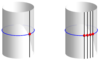
Figure 1: Sketch showing the first F-term, for a single magnon (left) and for a dyonic magnon (right). In the dyonic case (drawn as if $Q=4$ although in reality $Q\sim h\gg 1$) we attempt to show that the relevant S-matrix is constructed by fusion: $S_{1-Q}=\prod^{Q}S_{1-1}$.

2.2 Dyonic magnon F-term

The first step we take is to consider corrections to a dyonic magnon. This is a bound state of $Q\sim h\gg 1$ of the elementary particles of the same kind (taken to be of type A, and $a=1$), and it is the pole in $a_{1}$ at $y^{-}=x^{+}$ which allows the bound state to form. The constituent particles then have

$$x_{k}^{-}=x_{k-1}^{+},\qquad k=1,2,\ldots Q\,.$$

The relevant bound-state S-matrix is simply the product of the constituent S-matrices, which we illustrate as disjoint red balls in figure 1. It has the property that all dependence on the intermediate $x_{k}^{+}$ cancels out, leaving only $X^{-}=x_{1}^{-}$ and $X^{+}=x_{Q}^{+}$. (We review this construction in appendix B.3.) The result is

$$S_{b}(y^{\pm},X^{\pm})\equiv S_{1-Q}^{AA}(y^{\pm},X^{\pm})_{b1}^{b1} =\prod_{k=1}^{Q}S_{b}(y^{\pm},x_{k}^{\pm})$$

$$=s_{b}(y^{\pm},X^{\pm})\>S_{\mathrm{BDS}}(y^{\pm},X^{\pm})\>\sqrt{\frac{X^{+}}{X^{-}}}\left(\frac{y^{-}}{y^{+}}\right)^{Q/2}\sigma(y^{\pm},X^{\pm})$$

or, if the virtual particle is type B,

$$\tilde{S}_{b}(y^{\pm},X^{\pm})\equiv S_{1-Q}^{BA}(y^{\pm},X^{\pm})_{b1}^{b1}=s_{b}(y^{\pm},X^{\pm})\;\sqrt{\frac{X^{+}}{X^{-}}}\left(\frac{y^{-}}{y^{+}}\right)^{Q/2}\sigma(y^{\pm},X^{\pm})\,.\hphantom{\>S_{\mathrm{BDS}}(y^{\pm},X^{\pm})}$$

Then we want to evaluate the following sum:

$$e^{-iq_{\star}L}\sum_{b}(-1)^{F_{b}}(S_{b}+\tilde{S}_{b}) =e^{-iq_{\star}L}\left(S_{\mathrm{BDS}}+1\right)\left(s_{1}+s_{2}-s_{3}-s_{4}\right)\sqrt{\frac{X^{+}}{X^{-}}}\left(\frac{y^{-}}{y^{+}}\right)^{Q/2}\sigma(y^{\pm},X^{\pm})$$ (16)

$$=e^{-iq_{\star}L}\left(\frac{n^{2}}{\tilde{n}^{2}}+1\right)\left(1+\frac{\tilde{n}}{n}-2\tilde{n}\>e^{-ip/2}\right)e^{ip/2}\frac{1}{n}e^{-\frac{i}{h}\frac{x}{x^{2}-1}(E-Q/2)}+\mathcal{O}\Big{(}\frac{1}{h}\Big{)}$$

$$=F_{\mathrm{light}}^{(\ell=1)}+\mathcal{O}\Big{(}\frac{1}{h}\Big{)}$$

where we have used $y^{\pm}=x+\mathcal{O}(1/h)$ and that (11) still holds in the dyonic case.

This is the dyonic generalisation of the term calculated in [19], and the same result was also found by [22]. It matches the algebraic curve calculation we gave in [1].

2.3 Higher F-terms

By higher F-terms we mean those suppressed by

$$\left(e^{-\Delta/2h}\right)^{m},\qquad m=2,3,4\ldots\,.$$

Such Lüscher terms were studied in [29], where they arose from diagrams in which a virtual particle circles the cylinder twice (or $m$ times). The calculation performed there is a semiclassical mode sum, in which the mode $b$ has a phase shift $e^{i\delta_{ba}(k,p)}=S_{ba}^{ba}(k,p)$. To get the $m=2$ term, they use a cylinder of size $2L$ and a phase shift $2\delta$. Adding up all terms leads them to the following formula (their equation (33) or (3.8)):

$$\delta E=\frac{-1}{2\pi i}\fint_{-\infty}^{\infty}dq_{\star}\,\left[\varepsilon^{\prime}(q_{\star})-\varepsilon^{\prime}(p)\right]\sum_{b}(-1)^{F_{b}}\log\left(\frac{1-S_{b1}^{b1}(q_{\star},p)e^{-iq_{\star L}}}{1-e^{-iq_{\star L}}}\right).$$ (17)

Expanding this with $-\log\left(\frac{1-S\,e^{-L}}{1-e^{-L}}\right)=e^{-L}(S-1)+\frac{1}{2}e^{-2L}(S^{2}-1)+\frac{1}{3}e^{-3L}(S^{3}-1)+\ldots$ we write the $m$ component as

$$\delta E_{\mathrm{HJL}}^{F,m}=\frac{1}{2\pi}\fint_{-\infty}^{\infty}dq\,\left(1-\frac{\varepsilon^{\prime}(p)}{\varepsilon^{\prime}(q_{\star})}\right)e^{-miq_{\star}L}\frac{1}{m}\sum_{b}(-1)^{F_{b}}\left[S_{b1}^{b1}(q_{\star},p)^{m}-1\right].$$ (18)

Here we changed the integration variable, and also the contour — [29]’s derivation has $q_{\star}$ real, and we assume that this can be rotated back to imaginary in the same way as the $m=1$ term. Notice that we can drop the final $-1$ from this formula, since $\sum_{b}(-1)^{F_{b}}1=0$ as we have always equally many bosons and fermions.

To apply this result to $CP^{3}$ giant magnons, we should extend the sum over $b$ to also include whether the virtual particle is of type A or B. Then we obtain the following result, corresponding to the left half of figure 2:

$$e^{-2iq_{\star}L}\sum_{b=1}^{4}(-1)^{F_{b}}\left[(S_{b})^{2}+(\tilde{S}_{b})^{2}\right] =e^{-2iq_{\star}L}\left[a_{1}^{2}+(a_{1}+a_{2})^{2}-2(a_{6})^{2}\right]\left(n^{2}+\tilde{n}^{2}\right)(\sigma_{\mathrm{AFS}})^{2}$$

$$=e^{-2i\frac{\alpha\,x}{x^{2}-1}}4\left[a_{1}(x,x^{\pm})-1\right]+\mathcal{O}\Big{(}\frac{1}{h}\Big{)}.$$ (19)

The kinematic factor is the same as for the $m=1$ case, (12).

Now let us compare this to the algebraic curve calculation in [1], where we wrote:

$$\delta E_{\mathrm{new}}^{F} =-\frac{1}{4i}\oint_{\mathbb{U}}dx\sum_{ij}(-1)^{F_{ij}}\frac{q^{\prime}_{i}(x)-q^{\prime}_{j}(x)}{2\pi}\cot\Big{(}\frac{q_{i}(x)-q_{j}(x)}{2}\Big{)}\>\Omega_{ij}(x)$$ (20)

$$=\sum_{\ell=1,2,3\ldots}\frac{-1}{4\pi i}\sum_{\pm}\fint_{\mathbb{U}_{\pm}}dx\sum_{ij}(-1)^{F_{ij}}e^{\mp\ell i(q_{i}-q_{j})}\frac{1}{\ell}\partial_{x}\Omega_{ij}(x).$$ (21)

The terms in this sum are not the same as those in (18), because the heavy modes at $\ell$ contribute to $m=2\ell$. (This is because both $q_{i}$ and $q_{j}$ contribute to the pole at $x=\pm 1$, see (14), rather than just one for the light mode.) Thus the $m=1$ term checked in [1, 22] involves only the light modes, while the $m=2$ term involves also the heavy modes. We wrote this term as

$$\delta E^{F,2}=-\frac{1}{2\pi i}\fint_{\mathbb{U}_{+}}dx\left[\frac{1}{2}\;F_{\mathrm{light}}^{(\ell=2)}\;\Omega_{45}^{\prime}(x)+F_{\mathrm{heavy}}^{(\ell=1)}\;2\Omega_{45}^{\prime}(x)\right]$$ (22)

and had the following expressions for the $\sum_{ij}(-1)^{F_{ij}}e^{-\ell i(q_{i}-q_{j})}$ factor:

$$F_{\mathrm{light}}^{(\ell=2)}\Big{|}_{Q=1} =e^{-2i\frac{\alpha x}{x^{2}-1}}\frac{4(x^{2}-1)\left(e^{ip}-1\right)}{(x-e^{ip/2})^{2}}$$

$$F_{\mathrm{heavy}}^{(\ell=1)}\Big{|}_{Q=1} =e^{-2i\frac{\alpha x}{x^{2}-1}}\frac{(x+1)\left(e^{ip/2}-1\right)\left(e^{ip/2}(3+x)-(3x+1)\right)}{\left(x-e^{ip/2}\right)^{2}}\,.$$ (23)

It is easy to see that the term coming from the light modes alone matches the $m=2$ term from HJL, (18) above. (The factor $\frac{1}{2}$ in (22) is the $\frac{1}{m}$ in (18) of course. See section 2.6 for comparison at general $m$.) The term from the heavy modes requires a different explanation.

2.4 Heavy modes and virtual bound states

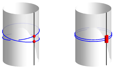
Figure 2: Sketch showing the second F-term for a single magnon. On the left is the contribution of a virtual particle circling the space twice, as in HJL, producing $(S_{1-1})^{2}$. On the right the contribution of a heavy mode (i.e. an $M=2$ bound state) for which we need $S_{2-1}$.

The sum over virtual particles in (3) should also run over all possible bound states. However the bound states we are interested in are those in the mirror theory, and because of this, we are interested in poles at $y^{+}=x^{-}$, rather than those at $y^{-}=x^{+}$ needed to build the dyonic magnon above.

In the ABJM case it is $\tilde{S}=S^{AB}$ which has these poles. We can read off the list of possible AB bound states from (55) – only $E_{11}^{11}$ and $E_{22}^{22}$ come with $a_{1}$ which cancels the pole from $\tilde{n}$. Thus we obtain the following list:

$$\begin{array}[]{rl}\mbox{bose+bose:}&\mbox{1+2}\\ \mbox{fermi+fermi:}&\mbox{3+3},\;\mbox{3+4},\;\mbox{4+4}\vspace{2mm}\\ \mbox{bose+fermi:}&\mbox{1+3},\;\mbox{1+4},\;\mbox{2+3},\;\mbox{2+4}\,.\end{array}$$ (24)

This is very similar to the off-shell construction of heavy modes in the algebraic curve, [40, 1], where again there is one heavy boson made from a pair of light bosons, and three made from a pair of fermions.

The first rather naive way to proceed is to use for S-matrix simply the product of those for the constituent light modes. This does lead us to the right answer:

$$e^{-2iq_{\star}L}\sum_{b+c=\mathrm{heavy}}(-1)^{F_{b+c}}S_{b}\tilde{S}_{c} =\left[a_{1}(a_{1}+a_{2})+3(a_{6})^{2}-2a_{1}a_{6}-2(a_{1}+a_{2})a_{6}\vphantom{\frac{1}{1}}\right]n\tilde{n}\>\sigma^{2}$$ (25)

$$=e^{-2i\frac{\alpha\,x}{x^{2}-1}}(a_{1}^{2}-4a_{1}+3)+\mathcal{O}\Big{(}\frac{1}{h}\Big{)}$$

$$=F_{\mathrm{heavy}}^{(\ell=1)}\Big{|}_{Q=1}+\ldots\,.$$

We have used here that the parameters of the constituents are all $y_{k}^{\pm}=x+\mathcal{O}(1/h)$, and thus $a_{i}$ simplify exactly as before, (10). In full, defining $x$ by (7) with $\pm M/2ih$ on the right, and taking $M=2$, the constituent points are

$$\begin{array}[]{ccccccccl}Y^{-}&\negthickspace\negthickspace=\negthickspace\negthickspace&y_{1}^{-}&&&&&=\negthickspace\negthickspace&x-\frac{ix^{2}}{h(x^{2}-1)}+\mathcal{O}(\frac{1}{h^{2}})\\ &&y_{1}^{+}&\negthickspace\negthickspace=\negthickspace\negthickspace&y_{2}^{-}&&&=\negthickspace\negthickspace&x\\ &&&&y_{2}^{+}&\negthickspace\negthickspace=\negthickspace\negthickspace&Y^{+}&=\negthickspace\negthickspace&x+\frac{ix^{2}}{h(x^{2}-1)}+\ldots\,.\end{array}$$ (26)

Using these the AFS dressing phase is the square of that in (11):

$$\sigma(y_{1}^{\pm},x^{\pm})\sigma(y_{2}^{\pm},x^{\pm})=\sigma(Y^{\pm},x^{\pm})=\left(\frac{x-1/x^{+}}{x-1/x^{-}}\right)^{2}e^{-\frac{2i}{h}\frac{x}{x^{2}-1}\left(E-\frac{Q}{2}\right)}+\mathcal{O}\Big{(}\frac{1}{h}\Big{)}.$$

Less naively, we should use the bound-state S-matrix $S_{2-1}(Y^{\pm},x^{\pm})_{b1}^{b1}$ derived by [27, 28]. The particular matrix elements we need are the same ones recently used in [41] (although here we turn off the $\beta$ twist factors), which correspond to the transfer matrix eigenvalues used in [42, 43]:

$$T_{M,1}^{SU(2)}=(-1)^{M}\left[(M+1)\,a_{5}^{5}+(M-1)\>2a_{8}^{8}-M\>a_{9}^{9}-M\,\frac{a_{9}^{9}+a_{3}^{3}}{2}\right].$$

Using the appropriate prefactors for ABJM (as reviewed in appendix B.4), we are led to the following expression, corresponding to the right half of figure 2:

$$e^{-2iq_{\star}L}\sum_{b=1}^{8}(-1)^{F_{i}^{i}}S_{b} =e^{-2iq_{\star}L}\left[\vphantom{\frac{1}{1}}3a_{5}^{5}+2a_{8}^{8}-2a_{9}^{9}-(a_{9}^{9}+a_{3}^{3})\right](x^{\pm},Y^{\pm})$$

$$\qquad\times n(y_{1}^{\pm},x^{\pm})\tilde{n}(y_{2}^{\pm},x^{\pm})\;\sigma(Y^{\pm},x^{\pm})$$

$$=F_{\mathrm{heavy}}^{(\ell=1)}\Big{|}_{Q=1}+\mathcal{O}\Big{(}\frac{1}{h}\Big{)}.$$

Note that while we are using the correct mirror–physical bound-state matrix elements here, we are still using a naive analytic continuation of the physical dressing phase $\sigma(x^{\pm},Y^{\pm})$ in order to evaluate it at this $Y^{\pm}$. This is commonly done for F-term calculations, as for instance in [19, 20, 21, 22], and it does give the correct answer here. We have also checked that the strong-coupling limit of the mirror–physical dressing phase computed in [44] reduces to this.

Kinetic factor

In (3) we are allowed to use two different dispersion relations for the real and the virtual particles. Since $y_{k}^{\pm}$ form a bound state, we should use for the virtual particle $\mathcal{E}(q_{\star})=\mathcal{E}_{M}(q_{\star})$. For clarity let us write this for general $M$, where we will have $Y^{\pm}=x\pm\frac{i\,M\,x^{2}}{2h(x^{2}-1)}+\mathcal{O}(\frac{1}{h^{2}})$ and thus

$$q_{\star}=\frac{M}{h}\frac{x}{x^{2}-1}+\mathcal{O}\Big{(}\frac{1}{h^{3}}\Big{)},\qquad q=\frac{i\,M}{2}\left(\frac{x^{2}+1}{x^{2}-1}\right)+\mathcal{O}\Big{(}\frac{1}{h^{2}}\Big{)}.$$

Then (9) is unchanged at this order:

$$\mathcal{E}^{\prime}(q_{\star})=h\frac{2x}{x^{2}+1}+\mathcal{O}\Big{(}\frac{1}{h}\Big{)}.$$

Define $\overline{q}_{\star}=q_{\star}/M$ and $\overline{q}=q/M$ , which are essentially the momentum and energy of each of the constituents of the virtual bound state. Then in terms of these, the on-shell condition can be re-written

$$q^{2}+\mathcal{E}(q_{\star})^{2}=0\quad\Rightarrow\quad\overline{q}^{2}+\varepsilon(\overline{q}_{\star})^{2}=0+\mathcal{O}\Big{(}\frac{M}{h^{2}}\Big{)}.$$

and thus $(i\overline{q},\overline{q}_{\star})$ describe a single on-shell particle, (4). We can now re-write the natural kinetic factor from (3) in terms of the new barred variables:

$$\fint dq\left(1-\frac{\epsilon^{\prime}(p)}{\mathcal{E}^{\prime}(q_{\star})}\right)e^{-i\,q_{\star}\,L}\ldots=\fint d\overline{q}\left(1-\frac{\epsilon^{\prime}(p)}{\varepsilon^{\prime}(\overline{q}_{\star})}\right)e^{-i\,M\overline{q}_{\star}\,L}\>M\times\ldots\,.$$ (27)

Now since $\overline{q}=\frac{1}{h}\frac{x}{x^{2}-1}$, we can drop the bar and combine this with the light mode integral, and then write this in terms of $x$ as before. The only new features are an overall factor of $M$, and $ML$ in the exponent, both of which are exactly what we wanted in order to match (22) when $M=2$.

Note, aside, that what we have written here would be equally true if we used for the virtual particle instead $\mathcal{E}(q_{\star})=M\varepsilon(q_{\star}/M)$. This is simply a superposition of two particles, like the $RP^{2}$ giant magnon.

2.5 Dyonic second F-term

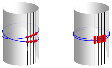
Figure 3: Sketch showing the second F-term for a dyonic magnon. For the light mode running in the loop (left) we need $(S_{1-Q})^{2}$. For a heavy mode running in the loop (right) we need $S_{2-Q}$, which we construct by fusion as $\prod^{Q}S_{2-1}$.

We can now extend this to allow the external particle to be a physical bound state, i.e. a dyonic giant magnon. We will still have the same two contributions, this time illustrated in figure 3. The first is from a fundamental virtual particle going around twice:

$$e^{-2iq_{\star}L}\sum_{b}(-1)^{F_{b}}\left[S_{b}(y^{\pm},X^{\pm})^{2}+\tilde{S}_{b}(y^{\pm},X^{\pm})^{2}\right]$$

$$=e^{-2iq_{\star}L}\left[(S_{\mathrm{BDS}})^{2}+1\vphantom{1^{1^{1}}}\right]\left[\vphantom{\frac{1}{1}}(s_{1})^{2}+(s_{2})^{2}-(s_{3})^{2}-(s_{4})^{2}\right]\frac{X^{+}}{X^{-}}\left(\frac{y^{-}}{y^{+}}\right)^{Q}\,\,\sigma^{2}(y^{\pm},X^{\pm})$$

$$=F_{\mathrm{light}}^{(\ell=2)}+\mathcal{O}\Big{(}\frac{1}{h}\Big{)}.$$

And the second contribution is from a virtual bound state running in the loop. For this last contribution, we need to derive $S_{2-Q}$ from $S_{2-1}$ by fusion. We give details of this in appendix B.5, and here simply write down the result:

$$e^{-2iq_{\star}L}\sum_{b=1}^{8}(-1)^{F}S_{b}(Y^{\pm},X^{\pm}) =T_{0}(y_{1}^{\pm},y_{2}^{\pm},X^{\pm})\left[3t_{1}+t_{4}-2t_{5}-2t_{7}\vphantom{1^{1^{1}}}\right]\sigma(Y^{\pm},X^{\pm})$$

$$=F_{\mathrm{heavy}}^{(\ell=1)}+\mathcal{O}\Big{(}\frac{1}{h}\Big{)}.$$ (28)

We did not explicitly show the results of the corresponding algebraic curve calculation in [1] for the dyonic case. They do however match the present calculation exactly. (We give all the necessary formulae in appendix C.)

2.6 All higher F-terms

It is possible to extend our results above to treat all higher F-terms. By doing so we can recover exactly the corresponding algebraic curve results. We do this using virtual elementary particles and two-particle ($M=2$) bound states.

What is not entirely clear to us is how, without knowing about the string theory, one would know to include $M=2$ but not for instance the $M=3,4$ virtual bound states. There is no obvious distinction visible from the S-matrix. Certainly adding such terms would spoil the agreement, starting with the 3rd F-term, because there are no corresponding modes in the algebraic curve (or in the worldsheet sigma-model) with mass 3 or 4. In the analogous $AdS_{5}\times S^{5}$ calculation one does not include any virtual bound states, and the analogous justification is to note that all modes of the string have mass 1.

Let us now state the results. We obtain agreement of $\delta E^{F,m}$ for all $m$ as follows:

• For odd $m$ the only contribution is from the light modes. Comparing (18) and (21), what we need is

  $$e^{-imq_{\star}L}\sum_{b=1}^{4}(-1)^{F_{b}}\left[(S_{b})^{m}+(\tilde{S}_{b})^{m}\right]\;\>=\;\>F_{\mathrm{light}}^{(m)}=\negthickspace\sum_{ij\,\mathrm{light}}(-1)^{F_{ij}}e^{-im(q_{i}-q_{j})}+\mathcal{O}\Big{(}\frac{1}{h}\Big{)}.$$

  This remains true if the physical particle is a dyonic magnon, interpreting $S_{b}$ as in (16).

• For even $m$ there is in addition a contribution from the heavy modes circling the space $\ell=m/2$ times. The agreement for this term comes from

  $$e^{-i\ell 2q_{\star}L}\sum_{b=1}^{8}(-1)^{F_{b}}(S_{b})^{\ell}\;\>=\;\>F_{\mathrm{heavy}}^{(\ell)}=\negthickspace\sum_{ij\,\mathrm{heavy}}(-1)^{F_{ij}}e^{-i\ell(q_{i}-q_{j})}+\mathcal{O}\Big{(}\frac{1}{h}\Big{)}.$$

  Here $e^{-im2q_{\star}L}$ is from (27), appropriately generalised. This agreement also holds for the dyonic case, where like (28) we use the mixed bound state S-matrix $S_{2-Q}$:

  $$e^{-i\ell 2q_{\star}L}T_{0}^{\ell}(y_{1}^{\pm},y_{2}^{\pm},X^{\pm})\left[3t_{1}^{\ell}+t_{4}^{\ell}-2t_{5}^{\ell}-2t_{7}^{\ell}\vphantom{1^{1^{1}}}\right]\sigma^{\ell}(Y^{\pm},X^{\pm})\;=\;F_{\mathrm{heavy}}^{(\ell)}+\mathcal{O}\Big{(}\frac{1}{h}\Big{)}.$$

  We can write the total correction at this order as

  $$\delta E^{F,m}=\frac{1}{2\pi}\fint_{-\infty}^{\infty}dq\,\left(1-\frac{\varepsilon^{\prime}(p)}{\varepsilon^{\prime}(q_{\star})}\right)\left[\frac{1}{m}F_{\mathrm{light}}^{(m)}+\frac{1}{m/2}2F_{\mathrm{heavy}}^{(m/2)}\right]+\mathcal{O}\Big{(}\frac{1}{h}\Big{)}.$$ (29)

Both of these expansions in $m$ come from exact formulae, (17) and (20). A convenient form in which to write the agreement to all orders is the following:

$$\prod_{b=1}^{4}\left[\left(1-S_{b}e^{-iq_{*}L}\right)\left(1-\tilde{S}_{b}e^{-iq_{*}L}\right)\right]^{(-1)^{F_{b}}} =\prod_{ij\,\mathrm{light}}\left[1-e^{-i(q_{i}-q_{j})}\right]^{(-1)^{F_{ij}}}+\mathcal{O}\Big{(}\frac{1}{h}\Big{)}$$ (30)

$$\prod_{b=1}^{8}\left[1-(S_{2-Q})_{b}e^{-iq_{*}L}\right]^{(-1)^{F_{b}}} =\prod_{ij\,\mathrm{heavy}}\left[1-e^{-i(q_{i}-q_{j})}\right]^{(-1)^{F_{ij}}}+\mathcal{O}\Big{(}\frac{1}{h}\Big{)}.$$ (31)

3 Lüscher $\mu$-term Corrections

In the field-theoretic derivation of the F-term formula (3), there is one diagram whose $\int dq$ contour must be moved by $ip_{0}$ before combining with the others. If this crosses any poles, they give rise to extra contributions, which are called $\mu$-terms. The generic formula is

$$\delta E^{\mu}=\operatorname{Re}\{\;-i\left(1-\frac{\varepsilon^{\prime}(p)}{\varepsilon^{\prime}(\tilde{q}_{\star})}\right)e^{-i\tilde{q}_{\star}L}\sum_{b}(-1)^{F_{b}}\mathop{\mathrm{Res}}_{q=\tilde{q}}\left[S_{ba}^{ba}(q_{\star}(q),p)-1\vphantom{\frac{1}{1}}\right]\}\,.$$ (32)

Not only are both real and virtual particles on-shell (as for the F-terms), but the loop momentum $q_{\mu}$ is now completely fixed to discrete values: $\tilde{q}$ is Euclidean energy at which there is a pole, and $\tilde{q}_{\star}$ is the corresponding momentum, given by (4).

The first calculation of $\mu$-terms for giant magnons was [12], recovering the classical finite-size corrections of [33, 45]. The dyonic version of this was studied by [31].

For magnons in $AdS_{4}\times CP^{3}$, classical $\mu$-terms have been studied by [20, 19, 21]. For the giant magnon in $RP^{2}$, these papers correctly recovered the AFZ correction [46, 2]. But for the elementary magnon (in $CP^{1}$) they obtained zero, apparently in contradiction with the string sigma-model [47, 48, 33]. The same zero result was also obtained by the first algebraic curve calculation [20], and this was shown to be an order-of-limits problem in [2], but to date this has not been resolved in the literature on Lüscher corrections.

We therefore compute $\mu$-terms for the dyonic elementary magnon, i.e. for the giant magnon solution in $CP^{2}$ of [2, 36]. We are able to recover the classical algebraic curve result of [2] for this correction. This classical term is the leading one in an expansion in $1/h$, and we go on to evaluate the formula (32) at the subleading order. Such a subleading term was calculated by [35] in $AdS_{5}\times S^{5}$ (where it was compared to a one-loop algebraic curve calculation) and by [19] for the case of the $RP^{2}$ giant magnon in $AdS_{4}\times CP^{3}$.

3.1 Setup

The pole in the S-matrix which normally gives rise to (32) is at $y^{-}=X^{+}$. To find the pieces we need, solve the equation $Q(y^{\pm})=1$ for $y^{+}$, to get

$$y^{+}=X^{+}+\frac{i}{h}\frac{X^{+2}}{X^{+2}-1}+\frac{1}{h^{2}}\frac{X^{+3}}{(X^{+2}-1)^{3}}+\mathcal{O}\Big{(}\frac{1}{h^{3}}\Big{)}.$$ (33)

Then the momentum of the virtual particle is

$$q_{\star}=-i\log\frac{y^{+}}{y^{-}} =\frac{1}{h}\frac{X^{+}}{X^{+2}-1}-\frac{i}{2h^{2}}\frac{X^{+2}(X^{+2}+1)}{(X^{+2}-1)^{3}}+\mathcal{O}\Big{(}\frac{1}{h^{3}}\Big{)}.$$ (34)

We will also need

$$q=\pm i\varepsilon^{\prime}(q_{\star}) =\pm\frac{i}{2}\frac{X^{+2}+1}{X^{+2}-1}\mp\frac{1}{h^{2}}\frac{X^{+3}}{(X^{+2}-1)^{3}}+\mathcal{O}\Big{(}\frac{1}{h^{2}}\Big{)}$$

$$\varepsilon^{\prime}(q_{\star}) =2h\frac{X^{+}}{X^{+2}+1}-i\frac{X^{+2}}{(X^{+2}+1)^{2}}+\mathcal{O}\Big{(}\frac{1}{h}\Big{)}$$

from which we get the kinetic factor to be

$$\left(1-\frac{\mathcal{E}^{\prime}_{Q}(p)}{\varepsilon^{\prime}(q_{\star})}\right)=-\frac{(X^{+}-X^{-})(X^{+2}-1)}{2X^{+}(X^{+}X^{-}+1)}-\frac{i}{4h}\frac{\;X^{+}+X^{-}}{(X^{+}X^{-}+1)}+\mathcal{O}\Big{(}\frac{1}{h^{2}}\Big{)}.$$ (35)

It is convenient to re-write the residue in terms of $y^{-}$ rather than $q$. Assuming that we have only a simple pole, the Jacobian factor which this change inserts is

$$\lim_{q\to\tilde{q}}\frac{q-\tilde{q}}{y^{-}(q)-X^{+}}=\frac{1}{\partial_{q}y^{-}}=\mp 2i\frac{X^{+}}{(X^{+2}-1)^{2}}\mp\frac{3}{h}\frac{X^{+2}(X^{+2}+1)}{(X^{+2}-1)^{4}}+\mathcal{O}\Big{(}\frac{1}{h^{2}}\Big{)}.$$ (36)

Putting these pieces into (32), and keeping just the leading term, we have:

$$\delta E^{\mu}=\operatorname{Re}\left\{e^{-L\frac{iX^{+}}{h(X^{+2}-1)}}\frac{(X^{-}-X^{+})}{(X^{+2}-1)(X^{+}X^{-}+1)}\mathop{\mathrm{Res}}_{Y^{-}=X^{+}}\sum_{b}(-1)^{F_{b}}S_{b}(y^{\pm},X^{\pm})\right\}.$$

In the case we study here there will also be a pole at $y^{+}=X^{+}$. For this pole, $y^{-}$ is given by

$$y^{-}=X^{+}-\frac{i}{h}\frac{X^{+2}}{X^{+2}-1}+\frac{1}{h^{2}}\frac{X^{+3}}{(X^{+2}-1)^{3}}+\mathcal{O}\Big{(}\frac{1}{h^{3}}\Big{)}$$

and the only change to the formulae above is to change the sign of the last term displayed for $q$, $q_{\star}$, the Jacobian and the kinetic factor. But $\varepsilon^{\prime}(q_{\star})$ is unchanged.

3.2 Leading $\mu$-term for the dyonic magnon

Using these pieces, we now wish to calculate (32) considering the real particle to be a dyonic giant magnon, and the virtual particle an elementary magnon. As for the corresponding F-term calculation (16), we are interested in

$$\sum_{b}(-1)^{F_{b}}S_{b}(y^{\pm},X^{\pm})=(S_{\mathrm{BDS}}+1)\left[s_{1}+s_{2}-s_{3}-s_{4}\right]\sqrt{\frac{X^{+}}{X^{-}}}\left(\frac{y^{-}}{y^{+}}\right)^{Q/2}\sigma\,.$$ (37)

This has poles at $y^{\pm}=X^{+}$ arising only from $S_{\mathrm{BDS}}$, (59). (Thus the only contribution is from when the virtual particle is type A.) We consider first the pole at $y^{-}=X^{+}$.

• The residue of $S_{\mathrm{BDS}}$, at point (33), is:

  $$\negthickspace\negthickspace\negthickspace\mathop{\mathrm{Res}}_{y^{-}=X^{+}}S_{\mathrm{BDS}}=\frac{h(X^{+2}-1)}{iX^{+2}}\frac{(X^{+}-X^{-})^{2}(1-\frac{1}{X^{+}X^{-}})^{2}}{(1-\frac{1}{X^{+2}})^{2}}+\frac{X^{+}(X^{+}-X^{-})(X^{+}X^{-}-1)}{X^{-}(X^{+2}-1)}+\mathcal{O}\Big{(}\frac{1}{h}\Big{)}.$$

  From the rest of $\hat{S}$ we need only $s_{1}=1$ at this order.

• The phases $\eta$ and the factor $e^{-iq_{\star}L}$ can be treated together [19]:

  $$\negthickspace\negthickspace e^{-iq_{\star}L}\sqrt{\frac{X^{+}}{X^{-}}}\left(\frac{y^{-}}{y^{+}}\right)^{Q/2} =e^{-iq_{\star}(L+\frac{Q}{2})}\sqrt{\frac{X^{+}}{X^{-}}}$$ (38)

  $$=e^{-\frac{i}{h}(L+\frac{Q}{2})\frac{X^{+}}{X^{+2}-1}}\sqrt{\frac{X^{+}}{X^{-}}}\left[1+\left(L+\frac{Q}{2}\right)\frac{X^{+2}(X^{+2}+1)}{2h^{2}(X^{+2}-1)^{3}}+\mathcal{O}\Big{(}\frac{1}{h^{2}}\Big{)}\right].$$

  Here we should note that this expansion appears to need to assume $L/h^{2}\ll 1$. (The same assumption was used in [19].) Of course for any Lüscher terms to be small corrections, we also need that $L/h\gg 1$. Note however that the term $L$ from here cancels out of the final correction $\delta E^{\mu}$, (44) below.

• The AFS dressing phase is

  $$\negthickspace\negthickspace\sigma_{\mathrm{AFS}}=e^{\frac{-X^{+}}{X^{+2}-1}\left(\frac{1}{X^{-}}-\frac{1}{X^{+}}\right)}\left[\frac{X^{-}(X^{+2}-1)}{X^{+}(X^{+}X^{-}-1)}-i\frac{(X^{+}-X^{-})(X^{+2}-2X^{-}X^{+}+1)}{2h(X^{+2}-1)^{2}(X^{+}X^{-}-1)^{2}}+\mathcal{O}\Big{(}\frac{1}{h^{2}}\Big{)}\right].$$ (39)

For the pole at $y^{+}=X^{+}$ the residue is exactly minus what we had above, and all other factors the same (at this order). Following the contour prescription of [31], this contribution enters with a minus, thus doubling the result. Then using $L=J/2=\Delta-E$, the final result can be written

$$\delta E_{\mathrm{class.}} =2\>\delta E_{\mathrm{class.}(y^{-}=X^{+})}$$

$$=\mbox{$\mp$}2ih\>e^{-\frac{i\Delta}{h}\frac{X^{+}}{X^{+2}-1}}\sqrt{\frac{X^{-}}{X^{+}}}\frac{(X^{+}X^{-}-1)(X^{+}-X^{-})^{3}}{X^{-2}(X^{+}X^{-}+1)(X^{+2}-1)}\,.$$ (40)

This exactly matches the algebraic curve result in [2], using $h=\sqrt{\lambda/2}=g/2$.

The choice of sign here, which comes from $q=\pm i\varepsilon(q_{\star})$, matches the factor $\cos(2\phi)$ seen in [2]. There $2\phi$ was interpreted as the geometric angle between adjacent magnons, incorporating what [49] called type (i) and type (ii) solutions.

3.3 Subleading $\mu$-term for the dyonic magnon

In order to determine the subleading (in $1/h$) contributions to the $\mu$-term, we already gave some expansions to more orders than required above. But there are extra contributions that only appear to this order, which are:

• The remainder of $\hat{S}$ (i.e. the supertrace of the $su(2|2)$ bound-state S-matrix) evaluated at (33) gives the following:

  $$\left[s_{1}+s_{2}-s_{3}-s_{4}\right]=1+\frac{i}{h}\frac{X^{+}}{X^{+}-X^{-}}\left(\frac{X^{-}}{X^{+}X^{-}-1}-\frac{2X^{+}}{X^{+2}-1}\sqrt{\frac{X^{-}}{X^{+}}}\right)+\mathcal{O}\Big{(}\frac{1}{h^{2}}\Big{)}.$$ (41)

  For the pole at $y^{+}=X^{+}$, this is instead exactly 1.

• The Hernandez–Lopez dressing phase [50] also contributes to the subleading term:

  $$\negthickspace\negthickspace\sigma_{\mathrm{HL}}=1+\frac{X^{+2}}{2h\pi(X^{+2}-1)}\left[\frac{-2}{X^{+2}-1}+\frac{(X^{-2}-1)}{(X^{+}-X^{-})(X^{+}X^{-}-1)}\log\frac{(X^{+}+1)(X^{-}-1)}{(X^{+}-1)(X^{-}+1)}\right]+\mathcal{O}\Big{(}\frac{1}{h^{2}}\Big{)}.$$ (42)

• The remainder of the dressing phase, $\sigma_{n\geq 2}$, does not contribute at this order; see below for comments.

The final result from the pole at $y^{-}=X^{+}$ is:

$$\delta E_{(y^{-}=X^{+})}=\delta E_{\mathrm{class.}(y^{-}=X^{+})}+\frac{i\,e^{\frac{i\,p}{2}}e^{-\frac{i\Delta}{h}\frac{X^{+}}{X^{+2}-1}}(X^{+}-X^{-})^{2}}{2(1+X^{-}X^{+})(X^{+2}-1)^{3}X^{-}}\Bigg{\{}4i\,e^{-\frac{i\,p}{2}}X^{+}(X^{+}X^{-}-1)(X^{+2}-1)$$

$$-i\,\left(4X^{+}+X^{+3}+X^{-2}X^{+}(1+4X^{+2})+2X^{-}(1-7X^{+2}+X^{+4})\right)$$

$$+\frac{X^{+}}{\pi}\left(2(X^{+}-X^{-})(X^{-}X^{+}-1)+(X^{-2}-1)(X^{+2}-1)\log\left[\frac{(X^{-}-1)(1+X^{+})}{(1+X^{-})(X^{+}-1)}\right]\right)$$

$$+\frac{\Delta}{h}\frac{X^{+}(X^{+}-X^{-})(X^{+}X^{-}-1)(1+X^{+2})}{(X^{+2}-1)}\Bigg{\}}$$ (43)

The pole at $y^{+}=X^{+}$ gives a similar contribution. Adding the two, and taking into account the sign as before,

$$\delta E_{(y^{-}=X^{+})}-\delta E_{(y^{+}=X^{+})}=\delta E_{\mathrm{class.}}+$$

$$\quad+\frac{e^{-\frac{i\Delta}{h}\frac{X^{+}}{X^{+2}-1}}(X^{+}-X^{-})^{2}}{X^{-}(X^{+2}-1)^{2}X^{+}(X^{+}X^{-}+1)}\Bigg{\{}-2X^{+}(X^{-}X^{+}-1)+e^{\frac{i\,p}{2}}X^{-}(X^{+2}-1)$$

$$+\frac{i\,e^{\frac{i\,p}{2}}}{\pi}\frac{X^{+}}{X^{-}(X^{+2}-1)}\left(2(X^{+}-X^{-})(X^{-}X^{+}-1)+\left(X^{-2}-1\right)\left(X^{+2}-1\right)\log\frac{(X^{-}-1)(1+X^{+})}{(1+X^{-})(X^{+}-1)}\right)\Bigg{\}}$$ (44)

which is the leading and subleading $\mu$-term corrections to the energy of the dyonic elementary magnon.

Let us make a two comments about the contribution of the dressing phase:

• Our calculation follows that of [31] in keeping only the AFS and HL phases, i.e. the terms $\chi$${}^{(n)}(x,y)/h^{n-1}$ for $n=0,1$ in (57). But if one considers the full sum infinite sum, the terms apparently subleading in $1/h$ can have non-trivial pole contributions, and thus contribute along with the earlier terms. Nevertheless, in the present dyonic case, if we perform a careful calculation of all the terms (following [12]), we find that the contribution from all higher terms does indeed vanish.

• However if we were to consider a non-dyonic magnon, i.e. to take $Q=1$ for the physical particle, then there would be contributions from $\sigma_{n\geq 2}$ both at leading and subleading orders. (This is also what happens in the calculation of [12].) Looking at $\sigma_{\mathrm{AFS}}$ (39), and likewise (41), (42), it seems that the non-dyonic limit of these expressions is ill defined, but in fact the divergences should cancel with extra terms that come from the taking the principal value in the $F$-term. See appendix A for a discussion of this subject in the $AdS_{5}\times S^{5}$ case.

4 F-terms for Composite Magnons

So far we have studied only the elementary giant magnon, and its dyonic generalisation. There are various other giant magnon solutions possible in $CP^{3}$, all of which are superpositions of two elementary magnons. From the sigma-model point of view this was shown by the dressing construction of [36]. They are of two kinds:

• The magnons in $RP^{2}$ and $RP^{3}$ are the same solutions as exist in $S^{2}$ [14] and $S^{3}$ [51], and the same is true of the corresponding finite-$J$ solutions [48]. This equivalence also holds to some degree in both algebraic curve and Lüscher calculations, where many formulae reduce to exactly what was used in $AdS_{5}\times S^{5}$.
  From the S-matrix point of view, the $RP^{2}$ magnon is a superposition of one A-particle and one B-particle, both with the same $su(2|2)$ label which we take to be $a=1$. In the dyonic case, these are each replaced by bound states of $Q$ particles.

• The so-called ‘big giant magnon’ is another superposition of two dyonic magnons, oriented such that their charges $Q$ cancel out. This was first known in the algebraic curve [52] and later constructed using dressing by [53, 54, 55]. The most explicit construction of it from two elementary magnons was given by [32], from which it is clear that the two particles carry different labels: say A with $a=1$, plus B with $a=2$.
  Classically, when $Q\to 1$ this becomes indistinguishable from the $RP^{2}$ solution (in both sigma-model and algebraic curve). We see this behaviour also for F-terms we calculate here. Even though they are corrections at order $h^{0}$ (while the classical energy is order $h$), they are the leading terms in $1/h$ in the coefficient $a_{m,0}$ of the exponential, (1) or (47).

We summarise all of the bound-state and composite magnons in table 1.

Physical Mirror Elementary Dyonic Composite $RP^{3}$ Composite ‘big’ Light Heavy $\vphantom{1^{1^{1}}}A_{a=1}$ $(A_{a=1})^{Q}$ $(A_{a=1}B_{a=1})^{Q}$ $(A_{a=1}B_{a=2})^{Q}$ $A_{a}$ and $B_{a}$ $(A_{a}B_{b})$ $a=1,2,3,4.$ $a,b$ as shown in (24).

Table 1: Summary of the various states considered, in spin-chain language. It would clearly be equivalent to consider corrections to, for instance, the $A_{a=2}$ physical particle or the $(B_{a=2})^{Q}$ dyonic magnon.

In [1] we did not write all of the the F-terms which we calculate here in full. But we give in appendix C enough formulae to check them.

4.1 The $RP^{3}$ magnon

Note that both constituent particles will always be described by the same $X^{\pm}$. We will use $p$, $E$, $Q$ and $J$ to be the quantities defined in terms of this in appendix B.1, even though the total momentum is then $p_{\mathrm{tot}}=2p$, total energy $2E$, and the total charge $2Q$ (or, for the big magnon, zero). This implies in particular that the kinetic factor will be unchanged: we have $E_{\mathrm{tot}}^{\prime}(p_{\mathrm{tot}})=\mathcal{E}^{\prime}_{Q}(p)$.

Allowing that the virtual particle may be A or B, the remaining factor of the integrand in (3) is the following:

$$e^{-iq_{\star}L}\sum_{b=1}^{4}(-1)^{F_{b}}\left[S_{b}\tilde{S}_{b}+\tilde{S}_{b}S_{b}\right](y^{\pm},x^{\pm}) =2\left[(a_{1})^{2}+(a_{1}+a_{2})^{2}-2(a_{6})^{2}\right]n\tilde{n}\sigma^{2}(y^{\pm},x^{\pm})$$

$$=4\,e^{-\frac{i}{h}\frac{x}{x^{2}-1}(2E-1-L)}\left[a_{1}(x,x^{\pm})^{2}-1\right]+\mathcal{O}\Big{(}\frac{1}{h}\Big{)}$$

$$=F_{\mathrm{light}[RP]}^{(\ell=1)}\Big{|}_{Q=1}+\ldots\,.$$

For $\sigma$ we use (11) above, and for all the other factors we are simply evaluating at $y^{\pm}=x$. For the exponents to match, we must remember that $\alpha=\Delta_{\mathrm{tot}}/h$ in the algebraic curve contains the total energy, $\Delta_{\mathrm{tot}}=2E-J$. And, following (15), we set $L$ to be half the total angular momentum:

$$L=J\,.$$

For the dyonic case (i.e. a superposition of two physical bound states, each with $Q$ particles) clearly we want instead:

$$e^{-iq_{\star}L}\sum_{b=1}^{4}(-1)^{F_{b}}\left[S_{b}\tilde{S}_{b}+\tilde{S}_{b}S_{b}\right](y^{\pm},X^{\pm}) =2\,S_{\mathrm{BDS}}\left[(s_{1})^{2}+(s_{2})^{2}-(s_{3})^{2}-(s_{4})^{2}\right]H^{2}\sigma^{2}(y^{\pm},X^{\pm})$$

$$=F_{\mathrm{light}[RP]}^{(\ell=1)}+\mathcal{O}\Big{(}\frac{1}{h}\Big{)}.$$

Here we write $H(y^{\pm},X^{\pm})=\sqrt{X^{+}/X^{-}}(y^{-}/y^{+})^{Q/2}$ for compactness, (60).

Second F-term

As for the elementary magnon, there are two terms which contribute to $\delta E^{F,2}$. One comes from a light mode (of type A or B) circling the space twice, what we called the HJL term (18). For this, (19) is replaced by

$$e^{-2iq_{\star}L}\sum_{b=1}^{4}(-1)^{F_{b}}\left[(S_{b}\tilde{S}_{b})^{2}+(\tilde{S}_{b}S_{b})^{2}\right](y^{\pm},x^{\pm}) =2\left[(a_{1})^{4}+(a_{1}+a_{2})^{4}-2(a_{6})^{4}\right](n\tilde{n})^{2}\sigma^{4}(y^{\pm},x^{\pm})$$

$$=4\,e^{-2\frac{i}{h}\frac{x}{x^{2}-1}(2E-1-L)}\left[a_{1}(x,x^{\pm})^{4}-1\right]+\mathcal{O}\Big{(}\frac{1}{h}\Big{)}$$

$$=F_{\mathrm{light}[RP]}^{(\ell=2)}\Big{|}_{Q=1}+\ldots$$

or, in the dyonic case,

$$e^{-2iq_{\star}L}\sum_{b=1}^{4}(-1)^{F_{b}}\left[(S_{b}\tilde{S}_{b})^{2}+(\tilde{S}_{b}S_{b})^{2}\right](y^{\pm},X^{\pm}) =2\,(S_{\mathrm{BDS}})^{2}\left[(s_{1})^{4}+(s_{2})^{4}-(s_{3})^{4}-(s_{4})^{4}\right]H^{4}\sigma^{4}(y^{\pm},X^{\pm})$$

$$=F_{\mathrm{light}[RP]}^{(\ell=2)}+\mathcal{O}\Big{(}\frac{1}{h}\Big{)}.$$

The other term comes from a heavy mode (or $M=2$ mirror bound state) running in the loop. Using the bound-state S-matrix $S_{2-1}$ we write

$$e^{-2iq_{\star}L}\sum_{b=1}^{8}(-1)^{F_{b}}S_{b}(Y^{\pm},x^{\pm})S_{b}(Y^{\pm},x^{\pm}) =\left[\vphantom{\frac{1}{1}}3(a_{5}^{5})^{2}+(2a_{8}^{8})^{2}-2(a_{9}^{9})^{2}-2\Big{(}\frac{a_{9}^{9}+a_{3}^{3}}{2}\Big{)}^{2}\right]n\tilde{n}\>\sigma^{2}(Y^{\pm},x^{\pm})$$

$$=F_{\mathrm{heavy}[RP]}^{(\ell=1)}\Big{|}_{Q=1}+\mathcal{O}\Big{(}\frac{1}{h}\Big{)}.$$

The dyonic version of this needs $S_{2-Q}$ as constructed in appendix B.5,

$$e^{-2iq_{\star}L}\sum_{b=1}^{8}(-1)^{F_{b}}S_{b}(Y^{\pm},X^{\pm})S_{b}(Y^{\pm},X^{\pm})$$

$$=e^{-2iq_{\star}L}(T_{0})^{2}\left[\vphantom{\frac{1}{1}}3(t_{1})^{2}+(t_{4})^{2}-2(t_{5})^{2}-2(t_{7})^{2}\right]\sigma^{2}(Y^{\pm},X^{\pm})$$

$$=e^{-\frac{i}{h}\frac{x}{x^{2}-1}(2E-Q-L)}\Big{[}3-2\left(\frac{x-X^{-}}{x-X^{+}}\sqrt{\frac{X^{+}}{X^{-}}}\right)^{2}+\left(\frac{(x-X^{-})(1-xX^{+})}{(x-X^{+})(1-xX^{-})}\right)^{2}-\left(\frac{1-xX^{+}}{1-xX^{-}}\sqrt{\frac{X^{-}}{X^{+}}}\right)^{2}\Big{]}+\ldots$$

$$=F_{\mathrm{heavy[RP]}}^{(\ell=1)}+\mathcal{O}\Big{(}\frac{1}{h}\Big{)}.$$

4.2 The big giant magnon

The only difference from the $RP^{3}$ case above is that one of the external particles is now $a=2$. Thus we will need for the first time matrix elements $S_{b2}^{b2}$. For the non-dyonic case these can be read off from (55) as follows:

$$\hat{S}_{b2}^{b2}=\hat{S}_{b^{\prime}1}^{b^{\prime}1},\qquad(b,b^{\prime})=(1,2),\>(2,1),\>(3,3),\>(4,4)\,.$$

Then we have

$$e^{-iq_{\star}L}\sum_{b=1}^{4}(-1)^{F_{b}}\left(S_{b1}^{b1}\tilde{S}_{b2}^{b2}+\tilde{S}_{b1}^{b1}S_{b2}^{b2}\right)(y^{\pm},x^{\pm}) =e^{-iq_{\star}L}2\left[a_{1}(a_{1}+a_{2})+(a_{1}+a_{2})a_{1}-2a_{6}a_{6}\right]n\tilde{n}\,\sigma^{2}$$

$$=F_{\mathrm{light}[\mathrm{Big}]}^{(\ell=1)}\Big{|}_{Q=1}+\mathcal{O}\Big{(}\frac{1}{h}\Big{)}.$$

This agrees with the $RP^{2}$ expression above.

For the dyonic case, we need the corresponding elements of $S_{Q-1}$. The above permutation clearly commutes with the fusion procedure used to construct this, and thus we have

$$e^{-iq_{\star}L}\sum_{b=1}^{4}(-1)^{F_{b}}\left(S_{b1}^{b1}\tilde{S}_{b2}^{b2}+\tilde{S}_{b1}^{b1}S_{b2}^{b2}\right)(y^{\pm},X^{\pm}) =2\,S_{\mathrm{BDS}}\left[s_{1}s_{2}+s_{2}s_{1}-s_{3}s_{3}-s_{4}s_{4}\right]H^{2}\sigma^{2}(y^{\pm},X^{\pm})$$

$$=F_{\mathrm{light}[\mathrm{Big}]}^{(\ell=1)}+\mathcal{O}\Big{(}\frac{1}{h}\Big{)}.$$

Second F-term

The term from a light mode wrapping twice is clearly given by

$$e^{-2iq_{\star}L}\sum_{b=1}^{4}(-1)^{F_{b}}\left[\left(S_{b1}^{b1}\tilde{S}_{b2}^{b2}\right)^{2}+\left(\tilde{S}_{b1}^{b1}S_{b2}^{b2}\right)^{2}\right](y^{\pm},x^{\pm})$$

$$=e^{-2iq_{\star}L}2\left[2(a_{1})^{2}(a_{1}+a_{2})^{2}-2(a_{6})^{4}\right](n\tilde{n})^{2}\sigma^{4}(y^{\pm},x^{\pm})$$

$$=F_{\mathrm{light}[\mathrm{Big}]}^{(\ell=2)}\Big{|}_{Q=1}+\mathcal{O}\Big{(}\frac{1}{h}\Big{)}$$

and for the dyonic case,

$$e^{-2iq_{\star}L}\sum_{b=1}^{4}(-1)^{F_{b}}\left[\left(S_{b1}^{b1}\tilde{S}_{b2}^{b2}\right)^{2}+\left(\tilde{S}_{b1}^{b1}S_{b2}^{b2}\right)^{2}\right](y^{\pm},X^{\pm})$$

$$=e^{-2iq_{\star}L}2(S_{\mathrm{BDS}})^{2}\left[(s_{1}s_{2})^{2}+(s_{2}s_{1})^{2}-(s_{3}s_{3})^{2}-(s_{4}s_{4})^{2}\right]H^{4}\sigma^{4}(y^{\pm},X^{\pm})$$

$$=F_{\mathrm{light}[\mathrm{Big}]}^{(\ell=2)}+\mathcal{O}\Big{(}\frac{1}{h}\Big{)}.$$

For the heavy mode, we need $S_{2-1}(Y^{\pm},x^{\pm})_{b2}^{b2}$. Here we make the following conjecture, based on the list of virtual bound states (24), and the S-matrix (62): under $a=1\leftrightarrow a=2$, the heavy boson $b=4$ is not mixed with the other three $b=1,2,3$. (These three all have the same $S_{b1}^{b1}$.) Meanwhile, the heavy fermions $b=5,6$ and $b=7,8$ are swopped. We can write this as the following permutation:

$$\hat{S}_{b2}^{b2}=\hat{S}_{b^{\prime}1}^{b^{\prime}1},\qquad b^{\prime}=\rho(b)\mbox{ where }\rho=(5,7)(6,8)\,.$$ (45)

Then using this, we are led to

$$e^{-2iq_{\star}L}\sum_{b=1}^{8}(-1)^{F_{b}}S_{b}(Y^{\pm},x^{\pm}) =\left[3(a_{5}^{5})^{2}+(2a_{8}^{8})^{2}-4a_{9}^{9}\frac{a_{9}^{9}+a_{3}^{3}}{2}\right]\,n\tilde{n}\>\sigma^{2}$$

$$=F_{\mathrm{heavy}[\mathrm{Big}]}^{(\ell=1)}\Big{|}_{Q=1}+\mathcal{O}\Big{(}\frac{1}{h}\Big{)}.$$

This conjecture follows through to the dyonic case, where in terms of $S_{2-Q}$ we have:

$$e^{-2iq_{\star}L}\sum_{b=1}^{8}(-1)^{F_{b}}\left(S_{b1}^{b1}\tilde{S}_{b2}^{b2}+\tilde{S}_{b1}^{b1}S_{b2}^{b2}\right)(Y^{\pm},X^{\pm})$$

$$=e^{-2iq_{\star}L}(T_{0})^{2}\left[3(t_{1})^{2}+(t_{4})^{2}-4(t_{5}t_{7})\right]\sigma^{2}(Y^{\pm},X^{\pm})$$

$$=e^{-\frac{i}{h}\frac{x}{x^{2}-1}(2E-Q-L)}\frac{(x^{2}-1)(X^{-}-X^{+})\left[x^{2}(3X^{-}-X^{+})+3X^{+}-X^{-}-2x(X^{-}X^{+}+1)\right]}{(xX^{-}-1)^{2}(x-X^{+})^{2}}+\ldots$$

$$=F_{\mathrm{heavy}[\mathrm{Big}]}^{(\ell=1)}+\mathcal{O}\Big{(}\frac{1}{h}\Big{)}.$$ (46)

The interpretation of the big giant magnon used here differs from that in [22]. There, it was treated as a superposition of a magnon and an ‘anti-magnon’, both of type A, with the latter defined by sending $X^{\pm}\to 1/X^{\mp}$ (so as to send $Q\to-Q$). This appears to give to the correct first and second F-terms: writing a prime for the ‘anti-magnon’, in the non-dyonic case these read:

$$F_{\mathrm{light}[\mathrm{Big}]}^{(\ell=1)}\Big{|}_{Q=1} =\left[a_{1}a_{1}^{\prime}+(a_{1}+a_{2})(a_{1}+a_{2}^{\prime})-2a_{6}a_{6}^{\prime}\right](nn^{\prime}+\tilde{n}\tilde{n}^{\prime})\sigma\sigma^{\prime}+\mathcal{O}\Big{(}\frac{1}{h}\Big{)}$$

$$F_{\mathrm{light}[\mathrm{Big}]}^{(\ell=2)}\Big{|}_{Q=1} =\left[(a_{1}a_{1}^{\prime})^{2}+(a_{1}+a_{2})^{2}(a_{1}+a_{2}^{\prime})^{2}-2(a_{6}a_{6}^{\prime})^{2}\right]\left[(nn^{\prime})^{2}+(\tilde{n}\tilde{n}^{\prime})^{2}\right](\sigma\sigma^{\prime})^{2}+\ldots$$

$$F_{\mathrm{heavy}[\mathrm{Big}]}^{(\ell=1)}\Big{|}_{Q=1} =\left[3a_{5}^{5}a_{5}^{5\prime}+4a_{8}^{8}a_{8}^{8\prime}-2a_{9}^{9}a_{9}^{9\prime}-(a_{9}^{9}+a_{3}^{3})(a_{9}^{9\prime}+a_{3}^{3\prime})\right]n\tilde{n}\>n^{\prime}\tilde{n}^{\prime}\,\sigma\sigma^{\prime}+\ldots\,.$$

All of these match the $RP^{2}$ magnon. In the dyonic case, we can recover the algebraic curve results if we use in the S-matrix for the ‘anti-magnon’ the following prefactor:

$$S_{\mathrm{BDS}}^{\prime}(y^{\pm},X^{\pm}) =S_{\mathrm{BDS}}(y^{\pm},1/X^{\mp})$$

Note however that this is not equal to $\prod_{k=1}^{Q}s_{\mathrm{BDS}}(y^{\pm},1/x_{k}^{\mp})$. In this calculation we evaluate the S-matrix at $y^{\pm}=y$; a more strict test of this interpretation could be obtained by performing a calculation in a regime where $y^{+}\neq y^{-}$, i.e. at the next order in $1/h$.

4.3 Agreement to all orders

As we noted for the elementary giant magnons in section 2.6, these results can be extended to recover all higher F-terms. The total contribution from elementary virtual particles matches that from the light modes in the algebraic curve, thanks to the following relations:

$$\prod_{b}\left[1-S_{b}\tilde{S}_{b}e^{-iq_{*}L}\right]^{(-2)^{F_{b}}} =\prod_{\stackrel{{\scriptstyle ij}}{{\mathrm{light[RP]}}}}\left[1-e^{-i(q_{i}-q_{j})}\right]^{(-1)^{F_{ij}}}+\mathcal{O}\Big{(}\frac{1}{h}\Big{)}$$

$$\prod_{b}\left[(1-S_{b1}\tilde{S}_{b2}e^{-iq_{*}L})(1-\tilde{S}_{b1}S_{b2}e^{-iq_{*}L})\right]^{(-1)^{F_{b}}} =\prod_{\stackrel{{\scriptstyle ij}}{{\mathrm{light[Big]}}}}\left[1-e^{-i(q_{i}-q_{j})}\right]^{(-1)^{F_{ij}}}+\mathcal{O}\Big{(}\frac{1}{h}\Big{)}.$$

The contribution from the virtual bound states (of only $M=2$ particles) similarly matches that from the heavy modes:

$$\prod_{b}\left[1-S_{b}(Y^{\pm},X^{\pm})e^{-2iq_{*}L}\right]^{(-2)^{F_{b}}} =\prod_{\stackrel{{\scriptstyle ij}}{{\mathrm{heavy[RP]}}}}\left[1-e^{-i(q_{i}-q_{j})}\right]^{(-1)^{F_{ij}}}+\mathcal{O}\Big{(}\frac{1}{h}\Big{)}$$

$$\prod_{b}\left[(1-S_{b1}\tilde{S}_{b2})(Y^{\pm},X^{\pm})e^{-2iq_{*}L})(1-\tilde{S}_{b1}S_{b2}(Y^{\pm},X^{\pm})e^{-2iq_{*}L})\right]^{(-1)^{F_{b}}}$$

$$=\prod_{\stackrel{{\scriptstyle ij}}{{\mathrm{heavy[Big]}}}}\left[1-e^{-i(q_{i}-q_{j})}\right]^{(-1)^{F_{ij}}}+\mathcal{O}\Big{(}\frac{1}{h}\Big{)}.$$

We have thus recovered the exact F-term (i.e. to all orders $m$) at one loop for all types of $CP^{3}$ giant magnon.

5 Conclusions

The complete energy of the giant magnon, including all exponential corrections, is given by [13]

$$E=\negthickspace\negthickspace\sum_{m,n=0,1,2\ldots}\negthickspace\negthickspace a_{m,n}\left(e^{-\Delta/2h}\right)^{m}\left(e^{-\Delta/E}\right)^{n}.$$ (47)

Here each coefficient $a_{m,n}$ is a function of the coupling. Our previous paper [1] calculated the infinite-volume term $a_{0,0}=\mathcal{E}_{Q}(p)$, as well as F-terms $a_{1,0}$ and $a_{2,0}$, at one loop in the string theory. We used the algebraic curve formulation, which exploits the integrability of the classical string theory, but is otherwise just a re-formulation of the sigma-model.

In this paper we have shown that, for Lüscher corrections, the heavy modes appearing in the string theory can be identified as bound states in the mirror theory. This allowed us to correctly recover the second F-term correction $a_{2,0}$ first computed in [1]. (The first F-term $a_{1,0}$ was also calculated by [52, 19] and for the dyonic case [22].) When treating dyonic giant magnons, we needed to scatter a physical bound state (of $Q$ particles) with a virtual bound state (of two), for which we were able to derive the appropriate S-matrix.

We have also computed $\mu$-term corrections for the elementary dyonic giant magnon. The leading term matches the classical finite-$J$ correction for this magnon, first given by [2]. We went on to compute the subleading term, giving a one-loop prediction. Since it comes from the all-loop S-matrix, this prediction is the second term in an expansion in $1/h(\lambda)$. This is related to the string theory’s coupling constant $\lambda\propto R^{2}/\alpha^{\prime}$ (at strong coupling) by

$$h(\lambda)=\sqrt{\frac{\lambda}{2}}+c+\mathcal{O}\Big{(}\frac{1}{\sqrt{\lambda}}\Big{)}.$$ (48)

Because the F-term corrections vanish classically (order $h\sim\sqrt{\lambda}$), their order $1$ terms are sensitive only to the leading term in the expansion (48). But, like the infinite-volume energy $a_{0,0}$, the one-loop part of the $\mu$-term is subleading in $1/h$. One extension which we hope to address in a forthcoming paper is the corresponding string theory calculation of $a_{0,1}$ at one loop, along the lines of [35].

Finally, we were also able to extenbd our calculation to obtain all higher F-terms $a_{m,0}$. In this calculation the elementary virtual particles contribute to every term via [29]’s generalised Lüscher formula (18), by circling the space $m$ times. The two-particle virtual bound states ($M=2$) contribute to even-numbered terms $m=2\ell$ in the same way. We did not include any bound states of $M\geq 3$ particles; this is natural from the algebraic curve perspective where one has modes of mass 1 and 2 only, but does not seem obvious from the S-matrix (see section 2.6).

In order to understand this better, a possible connection of these Lüscher corrections with the asymptotic solution of the $AdS_{4}/CFT_{3}$ TBA/Y-system proposed in [56, 57] is currently under investigation. It would be very interesting to understand from this how the F-terms involving all bound states at weak coupling re-sum to involve only $M=1,2$ at strong coupling.

Acknowledgements

We have benefitted greatly from conversations with Changrim Ahn, Zoltan Bajnok, Davide Fioravanti, Minkyoo Kim, Rafael Nepomechie, and especially with Olof Ohlsson Sax, and it is a pleasure to thank them all. We would also like to thank a J. Phys. A referee for some very useful comments.

For hospitality while working on this, we thank the Perimeter Institute, Nordita, and Humboldt University Berlin. I. Aniceto was partly funded by Fundação para a Ciência e Tecnologia, fellowship SFRH/BPD/69696/2010. D. Bombardelli was partly funded by Fundação para a Ciência e Tecnologia, fellowship SFRH/BPD/69813/2010, and also by the network UNIFY for travel support.

Appendix A $\mu$-terms for the $AdS_{5}\times S^{5}$ Giant Magnon

We show here the analogue in $AdS_{5}\times S^{5}$ of our calculation of the $\mu$-terms for a dyonic giant magnon in $AdS_{4}\times CP^{3}$ in section 3.3.

The dispersion relation for this theory is as follows:

$$\Delta-J=\mathcal{E}^{AdS_{5}}(p) =\sqrt{Q^{2}+\frac{\lambda}{\pi^{2}}\sin^{2}\frac{p}{2}}$$

$$=2\mathcal{E}_{Q}(p)\qquad\qquad\qquad\qquad\mbox{with }h=\smash{\frac{\sqrt{\lambda}}{4\pi}}$$

$$=-ih\left(X^{+}-\frac{1}{X^{+}}-X^{-}+\frac{1}{X^{-}}\right).$$

With this identification of $h$ and of $\mathcal{E}^{AdS_{5}}$ we can now re-use all of our expressions from section 3.1, multiplying $q$ and thus the Jacobian factor (36) by 2. (But leaving the kinetic term (35) unchanged.)

The important difference is the S-matrix involved, from which instead of (37) we should use:

$$\sum_{b}S_{b}(y^{\pm},X^{\pm}) =S_{\mathrm{BDS}}\left[s_{1}+s_{2}-s_{3}-s_{4}\right]^{2}\>\frac{X^{+}}{X^{-}}\left(\frac{y^{-}}{y^{+}}\right)^{Q}\sigma^{2}\,.$$ (49)

All the pieces of this are the same as we used above. Adding the contributions at both poles $y^{\pm}=X^{+}$, we get the following leading correction:

$$\delta E_{\mathrm{class.}}=\frac{2ih}{X^{+}X^{-}}\frac{(X^{+}-X^{-})^{3}}{(X^{+}X^{-}+1)}e^{\frac{X^{+}}{X^{+2}-1}\left(\frac{i}{h}L+\frac{i}{h}Q+\frac{2}{X^{+}}-\frac{2}{X^{-}}\right)}.$$

This is exactly the term given by [31].

Going to the next order, the contribution from the pole $y^{-}=X^{+}$ is this:

$$\delta E_{(y^{-}=X^{+})} =\delta E_{\mathrm{class.}(y^{-}=X^{+})}+\frac{4(X^{+}-X^{-})^{2}e^{ip-i\frac{\Delta X^{+}}{h(X^{+2}-1)}}}{(X^{+}X^{-}+1)((X^{+})^{2}-1)^{2}}\left[-2e^{-i\frac{p}{2}}(X^{+2}-1)+i\frac{X^{+}-X^{-}}{\pi}\right.$$

$$\qquad\frac{X^{+}+X^{-}(1+X^{+2}(-4+X^{+}(X^{-}+X^{+})))}{X^{+}(X^{+}X^{-}-1)}+i\frac{\Delta}{4h}\frac{(X^{+2}+1)(X^{+}-X^{-})}{X^{+}-1}$$

$$\qquad\left.+\frac{i((X^{-})^{2-1})(X^{+2}-1)}{2\pi(X^{+}X^{-}-1)}\log\frac{(X^{-}-1)(X^{+}+1)}{(X^{-}+1)(X^{+}-1)}\right].$$

The contribution from the pole at $y^{+}=X^{+}$ is similar, and adding them (with the same minus as before)

$$\negthickspace\negthickspace\delta E_{(y^{-}=X^{+})}-\delta E_{(y^{+}=X^{+})}=\delta E_{\mathrm{class.}}+\mbox{Re}\Bigg{\{}\frac{4(X^{+}-X^{-})^{2}e^{ip-i\frac{\Delta X^{+}}{h((X^{+})^{2}-1)}}}{(X^{+}X^{-}+1)(X^{+2}-1)^{2}}\left[\frac{X^{-}(X^{+2}-1)^{2}}{X^{+}(X^{+}X^{-}-1)}\right.$$

$$\left.-2e^{-i\frac{p}{2}}((X^{+})^{2}-1)+2i\frac{X^{+}-X^{-}}{\pi}+\frac{i((X^{-})^{2-1})((X^{+})^{2}-1)}{\pi(X^{+}X^{-}-1)}\log\frac{(X^{-}-1)(X^{+}+1)}{(X^{-}+1)(X^{+}-1)}\right]\Bigg{\}}.$$ (50)

Naively the non-dyonic limit of this diverges, giving:

$$\delta E^{\mu}=-16e^{-\frac{J}{2h\sin\frac{p}{2}}-2}\left[h\sin^{3}\frac{p}{2}+\frac{h\sin\frac{p}{2}}{Q}+\frac{\sin\frac{p}{2}}{\pi}\right].$$

However there is another contribution from the fact that a pole in the F-term integral at $x=X^{+}$ approaches the integration contour:

$$\delta E^{F} =\fint_{\mathbb{U}_{+}}dx\frac{2i\>x}{\pi(x^{2}-1)^{2}}\left(1-\frac{\mathcal{E}^{\prime}(p)}{\varepsilon^{\prime}(q_{*})}\right)e^{-\frac{i\Delta x}{h(x^{2}-1)}}\left(e^{i\frac{p}{2}}\frac{x-X^{-}}{x-X^{+}}+e^{i\frac{p}{2}}\frac{x-1/X^{+}}{x-1/X^{-}}-2\right)^{2}$$

$$\to\fint_{\mathbb{U}_{+}}dx\frac{2i\>x}{\pi(x^{2}-1)^{2}}\left(1-\frac{\mathcal{E}^{\prime}(p)}{\varepsilon^{\prime}(q_{*})}\right)e^{-\frac{i\Delta x}{h(x^{2}-1)}}\left(2e^{i\frac{p}{2}}\frac{x-1/x^{+}}{x-x^{+}}-2\right)^{2}$$

$$\qquad+e^{-\frac{J}{2h\sin\frac{p}{2}}-2}\left(-\frac{16h\sin^{3}\frac{p}{2}}{Q}+\frac{4iJ\cos\frac{p}{2}}{h}-8i\sin\frac{p}{2}+8i\sin p\right)+\mathcal{O}\Big{(}\frac{1}{h}\Big{)}.$$

This clearly cancels the $1/Q$ term, and taking the real part we get the following total non-dyonic correction:

$$\delta E=-16\,e^{-\frac{J}{2h\sin\frac{p}{2}}-2}\left[h\sin^{3}\frac{p}{2}+\frac{\sin\frac{p}{2}}{\pi}+\mathcal{O}\Big{(}\frac{1}{h}\Big{)}\right].$$ (51)

This agrees with the Lüscher correction calculated by [35] by considering the non-dyonic case from the beginning. This is a nontrivial agreement as in that case there are contributions from higher terms in the dressing phase $\sigma_{n\geq 2}$, which did not enter into our derivation of the the dyonic case above.

This non-dyonic subleading term (51) also matches the real part of the algebraic curve result in [35]. (The real part would be obtained there if one included also the contributions in the lower half-plane.) However the dyonic subleading term (50) differs from the algebraic curve result of [35].

Appendix B Two-particle and bound-state S-matrices

In this appendix we collect familiar formulae for magnons and their S-matrix. We discuss a number of kinds of bound-state S-matrices: $S_{1-Q}$ ($Q\sim h$ physical), $S_{M-1}$ ($M\sim 1$ virtual), and $S_{M-Q}$ (mixed).

B.1 Parameters

We describe magnons using Zhukovsky variables (in the complex spectral plane) which are defined in terms of the charge $Q$ and momentum $p$ by

$$Q(X^{\pm}) =-ih\left(X^{+}+\frac{1}{X^{+}}-X^{-}-\frac{1}{X^{-}}\right)$$ (52)

$$p =-i\>\log\frac{X^{+}}{X^{-}}$$

or, solving for $X^{\pm}$,

$$X^{\pm}=e^{\pm ip/2}\frac{\frac{Q}{2}+\sqrt{\frac{Q^{2}}{4}+4\,h^{2}\>\sin^{2}\frac{p}{2}}}{2h\>\sin\frac{p}{2}}\,.$$

The dispersion relation can be written in terms of these:

$$E =\mathcal{E}_{Q}(p)=\sqrt{\frac{Q^{2}}{4}+4\,h^{2}\>\sin^{2}\frac{p}{2}}$$ (53)

$$=-i\frac{h}{2}\left(X^{+}-\frac{1}{X^{+}}-X^{-}+\frac{1}{X^{-}}\right).$$

We will need the derivative of this with respect to $p$, holding $Q$ fixed, which can be written as

$$\mathcal{E}_{Q}^{\prime}(p)=h\frac{X^{+}+X^{-}}{X^{+}X^{-}+1}\,.$$ (54)

While we have given these initial formulae for the general dyonic case, we will discuss first the case of just one magnon, $Q=1$, for which we use lower-case $x^{\pm}$ and $\varepsilon(p)$. Then we can expand in $1/h$ to write:

$$\varepsilon(p) =2h\,\sin\frac{p}{2}+\mathcal{O}\Big{(}\frac{1}{h}\Big{)}$$

$$\varepsilon^{\prime}(p) =h\,\cos\frac{p}{2}+\mathcal{O}\Big{(}\frac{1}{h}\Big{)}$$

$$x^{\pm} =e^{\pm ip/2}\left[1+\frac{1}{4h\,\sin\frac{p}{2}}+\mathcal{O}\Big{(}\frac{1}{h^{2}}\Big{)}\right].$$

B.2 Two-particle S-matrix

Now consider two particles $x^{\pm}$ and $y^{\pm}$. The ABJM S-matrix is [17]

$$S(y^{\pm},x^{\pm}) \;=S_{AA}=S_{BB}\;=\hat{S}\>n\,\sigma$$

$$\tilde{S}(y^{\pm},x^{\pm}) \;=S_{AB}=S_{BA}\;=\hat{S}\>\tilde{n}\,\sigma\,.$$

with the same $su(2|2)$ invariant matrix part $\hat{S}$ [7, 9] as the SYM case, but one less power of the BES dressing phase $\sigma$ [37]. Explicitly, in our notation the SYM case has:

$$S=\hat{S}\otimes\hat{S}\>n\tilde{n}\,\sigma^{2}\,.$$

The factors which distinguish particles of type A and B [17] we have named $n$ and $\tilde{n}$:

$$n(y^{\pm},x^{\pm})=\frac{1-\frac{1}{y^{+}x^{-}}}{1-\frac{1}{y^{-}x^{+}}},\qquad\tilde{n}(y^{\pm},x^{\pm})=\frac{y^{-}-x^{+}}{y^{+}-x^{-}}\,.$$

Note of course that $\tilde{n}(y^{\pm},x^{\pm})=1/\tilde{n}(x^{\pm},y^{\pm})=1/\tilde{n}(y^{\mp},x^{\mp})$ and similarly for $n(y^{\pm},x^{\pm})$.

The relevant terms of the matrix part are given by [9]

$$\hat{S} =a_{1}\left(E_{11}^{11}+E_{22}^{22}+E_{12}^{12}+E_{21}^{21}\right)+a_{2}\left(E_{12}^{12}+E_{21}^{21}\right)$$

$$+a_{3}\left(E_{33}^{33}+E_{44}^{44}+E_{34}^{34}+E_{43}^{43}\right)+a_{4}\left(E_{34}^{34}+E_{43}^{43}\right)$$

$$+a_{5}\left(E_{13}^{13}+E_{14}^{14}+E_{23}^{23}+E_{24}^{24}\right)$$

$$+a_{6}\left(E_{31}^{31}+E_{41}^{41}+E_{32}^{32}+E_{42}^{42}\right)\qquad+\mbox{ terms }E_{ab}^{ba}\,.$$ (55)

Particles $b=1,2$ are bosons, and $b=3,4$ here are fermions. The coefficients are:

$$a_{1}(y^{\pm},x^{\pm}) =\frac{y^{+}-x^{-}}{y^{-}-x^{+}}\;\sqrt{\frac{x^{+}}{x^{-}}}\>\sqrt{\frac{y^{-}}{y^{+}}} a_{3}(y^{\pm},x^{\pm}) =-1$$

$$a_{2}(y^{\pm},x^{\pm}) =\frac{(y^{-}-y^{+})(x^{-}-x^{+})(x^{-}+y^{+})}{(y^{-}-x^{+})(x^{-}y^{-}-x^{+}y^{+})}\;\sqrt{\frac{x^{+}}{x^{-}}}\>\sqrt{\frac{y^{-}}{y^{+}}} a_{4}(y^{\pm},x^{\pm}) =a_{2}(x^{\mp},y^{\mp})$$ (56)

$$a_{6}(y^{\pm},x^{\pm}) =\frac{y^{+}-x^{+}}{y^{-}-x^{+}}\;\sqrt{\frac{y^{-}}{y^{+}}} a_{5}(y^{\pm},x^{\pm}) =a_{6}(x^{\mp},y^{\mp})\,.$$

We have assumed (as we will always do) that we are in the string frame. This has produced the square-root factors, which are the phases $\eta$, often written

$$\frac{\eta_{1}}{\tilde{\eta}_{1}}=\sqrt{\frac{x^{+}}{x^{-}}}=e^{ip/2},\qquad\frac{\eta_{2}}{\tilde{\eta}_{2}}=\sqrt{\frac{y^{-}}{y^{+}}}=e^{-i\,q_{\star}/2}.$$

The alternative is the spin chain frame, which sets both of these to 1. We observe that in this case, we have exactly $a_{1}=1/\tilde{n}$.

The BES dressing phase is

$$\sigma(y^{\pm},x^{\pm})=\exp\left[i\chi(y^{-},x^{-})-i\chi(y^{-},x^{+})-i\chi(y^{+},x^{-})+i\chi(y^{+},x^{+})\vphantom{1_{1_{1}}^{1^{1}}}\right].$$ (57)

Expanding $\chi=\sum_{n=0}^{\infty}\chi^{(n)}/h^{n-1}$, the leading term gives the AFS phase, and takes the simple form

$$\chi^{(0)}(y,x)=h\left(\frac{1}{y}-\frac{1}{x}\right)\left[1-(1-xy)\log\left(1-\frac{1}{xy}\right)\right].$$

The next term $\chi^{(1)}$ gives the HL phase. Writing $\chi(x,y)=\tilde{\chi}(x,y)-\tilde{\chi}(y,x)$, this is given by

$$\tilde{\chi}^{(1)}(x,y) =\frac{1}{2\pi}\mathrm{Li}_{2}\left(1-\frac{x+1}{x-1}\frac{y-1}{y+1}\right)-\frac{1}{2\pi}\mathrm{Li}_{2}\left(1-\frac{x+1}{x-1}\frac{y-1}{y+1}e^{i\pi}\right)$$

$$\quad-\frac{i}{2}\mathrm{Log}\left(1-\frac{x+1}{x-1}\frac{y-1}{y+1}e^{i\pi}\right)+\frac{\pi}{8}+\frac{1}{2\pi}\left[\mathrm{Li}_{2}(y)-\mathrm{Li}_{2}(-y)-\mathrm{Li}_{2}(x)+\mathrm{Li}_{2}(-x)\right].$$

The expressions for subsequent terms $\chi^{(n)}$ $n\geq 2$ can be found in [12].

B.3 Physical bound states: $S_{1-Q}$

If two bosonic particles are of the same type, then in $S^{AA}$ we have a factor $a_{1}$, which has a pole at $y^{-}=x^{+}$. This pole is what is used to build the bound states corresponding to dyonic giant magnons. The spectral parameters of the constituent particles are then connected up like this:

$$x_{k}^{\pm},\quad k=1,2\ldots Q\qquad\mbox{ with }\;x_{k}^{-}=x_{k-1}^{+}\,.$$ (58)

From (53) it is easy to see that in the total energy, all intermediate $x_{k}^{\pm}$ cancel out, leaving only

$$X^{+}=x_{Q}^{+},\qquad X^{-}=x_{1}^{-}\,.$$

The total charge $Q$ and momentum $p$ are likewise given in terms of these capital spectral parameters by (52).

The S-matrix for scattering of one particle ‘$b$’ off of this bound state is simply the product of the S-matrices with each constituent particle:

$$S_{1-Q}(y,X)_{b1}^{b1}=\prod_{k=1}^{Q}S(y,x_{k})_{b1}^{b1}\,.$$

Fortunately some similar cancellations happen here, again removing dependence on the individual $x_{k}$. Consider first the case of AA scattering, for which

$$S^{AA}(y^{\pm},x^{\pm})_{11}^{11}=\frac{n}{\tilde{n}}\>\sqrt{\frac{x^{+}}{x^{-}}}\sqrt{\frac{y^{-}}{y^{+}}}\>\sigma=s_{0}\,\sigma\,.$$

The factor $s_{\mathrm{BDS}}=n/\tilde{n}$ also appears in the SYM case in $S_{(11)(11)}^{(11)(11)}=(a_{1})^{2}n\tilde{n}\,\sigma^{2}$. It has the following cancellation property:

$$\prod_{k=1}^{Q}s_{\mathrm{BDS}}(y^{\pm},x_{k}^{\pm}) =\prod_{k=1}^{Q}\frac{n(y^{\pm},x_{k}^{\pm})}{\tilde{n}(y^{\pm},x_{k}^{\pm})}$$

$$=\frac{(y^{+}-X^{-})(1-\frac{1}{y^{+}X^{-}})}{(y^{-}-X^{+})(1-\frac{1}{y^{-}X^{+}})}\frac{(y^{-}-X^{-})(1-\frac{1}{y^{-}X^{-}})}{(y^{+}-X^{+})(1-\frac{1}{y^{+}X^{+}})}\equiv S_{\mathrm{BDS}}(y^{\pm},X^{\pm})\,.$$ (59)

Here we must use $Q=1$ for $x_{k}^{\pm}$ and $y^{\pm}$. More obviously, we have

$$\prod_{k=1}^{Q}\sqrt{\frac{x_{k}^{+}}{x_{k}^{-}}}\sqrt{\frac{y^{-}}{y^{+}}}=\sqrt{\frac{X^{+}}{X^{-}}}\left(\frac{y^{-}}{y^{+}}\right)^{Q/2}\equiv H(y^{\pm},X^{\pm})\,.$$ (60)

and for the dressing factor, the antisymmetry $\chi(y,x)=-\chi(x,y)$ leads to another cancellation:

$$\prod_{k=1}^{Q}\sigma(y^{\pm},x_{k}^{\pm})=\sigma(y^{\pm},X^{\pm})\,.$$

We must still consider matrix elements other than $S^{AA}(y^{\pm},x^{\pm})_{11}^{11}$. If we define

$$s_{b}\equiv\prod_{k=1}^{Q}\frac{\hat{S}_{b1}^{b1}}{\hat{S}_{11}^{11}}\,.$$

then obviously $s_{1}=1$, and some similar cancellations lead to [31]

$$s_{2} =\frac{(y^{+}-X^{+})(1-\frac{1}{y^{-}X^{+}})}{(y^{+}-X^{-})(1-\frac{1}{y^{-}X^{-}})}$$

$$s_{3}=s_{4} =\frac{y^{+}-X^{+}}{y^{+}-X^{-}}\sqrt{\frac{X^{-}}{X^{+}}}.$$

Finally, considering also AB scattering, it is clear that to change the prefactor from $n$ to $\tilde{n}$ you divide by $s_{\mathrm{BDS}}$, removing that factor. All together, the final S-matrix is given by

$$S_{1-Q}^{AA}(y^{\pm},X^{\pm})_{b1}^{b1}=S_{1-Q}^{BB}(y^{\pm},X^{\pm})_{b1}^{b1} =s_{b}\>S_{\mathrm{BDS}}\>H\>\sigma$$

$$S_{1-Q}^{AB}(y^{\pm},X^{\pm})_{b1}^{b1}=S_{1-Q}^{BA}(y^{\pm},X^{\pm})_{b1}^{b1} =s_{b}\>H\>\sigma\,.$$

with $b=1,2,3,4$.

From this S-matrix, we can get some elements of $S_{Q-1}$ by the following symmetry:

$$S_{Q-1}(Y^{\pm},x^{\pm})_{ba}^{ba}=S_{1-Q}(x^{\mp},Y^{\mp})_{ab}^{ab}\,.$$ (61)

Note however that we will only have $S_{Q-1}(Y^{\pm},x^{\pm})_{1a}^{1a}$, since we started with one particular bound state of $Q$ particles. And further that this is a physical bound state. Some $S_{Q-Q^{\prime}}(Y^{\pm},X^{\pm})$ bound-state S-matrices were constructed by [32], for the scattering of two physical dyonic giant magnons. However for scattering involving bound states of virtual particles, we need something different.

B.4 Mirror bound states: $S_{M-1}$

For a bound state of $M$ particles, [41] give (twisted generalisations of) these S-matrix elements:

$$(-1)^{F_{b}}\hat{S}_{M-1}(Y^{\pm},x^{\pm})_{b1}^{b1}=\begin{cases}a_{5}^{5}(x^{\pm},Y^{\pm}),\qquad&b=1,\ldots,M+1\\ 2a_{8}^{8}&b=M+2,\ldots,2M\\ (-1)\>a_{9}^{9}&b=2M+1,\ldots,3M\\ (-1)\>\dfrac{a_{9}^{9}+a_{3}^{3}}{2}&b=3M+1,\ldots,4M\,.\end{cases}$$ (62)

The coefficients are from [58], which we write at once in the string frame:

$$a_{5}^{5}(x^{\pm},Y^{\pm}) =\frac{x^{+}-Y^{+}}{x^{+}-Y^{-}}\sqrt{\frac{Y^{-}}{Y^{+}}}$$

$$a_{8}^{8}(x^{\pm},Y^{\pm}) =\frac{x^{-}(x^{-}-Y^{+})(1-x^{+}Y^{-})}{2x^{+}(x^{+}-Y^{-})(1-x^{-}Y^{-})}\sqrt{\frac{Y^{-}}{Y^{+}}}\frac{x^{+}}{x^{-}}$$

$$a_{9}^{9}(x^{\pm},Y^{\pm}) =\frac{x^{-}-Y^{+}}{x^{+}-Y^{-}}\sqrt{\frac{Y^{-}}{Y^{+}}}\sqrt{\frac{x^{+}}{x^{-}}}$$

$$a_{3}^{3}(x^{\pm},Y^{\pm}) =\frac{x^{-}x^{+}(1+x^{-}Y^{-}-2x^{+}Y^{-})+\left(x^{+}+x^{-}(-2+x^{+}Y^{-})\right)}{x^{+}(x^{+}-Y^{-})(1-x^{-}Y^{-})}Y^{+}\sqrt{\frac{Y^{-}}{Y^{+}}}\sqrt{\frac{x^{+}}{x^{-}}}$$

$$\Rightarrow\quad\frac{a_{3}^{3}+a_{9}^{9}}{2}=\frac{(x^{+}-Y^{+})(x^{+}Y^{-}-1)}{(x^{+}-Y^{-})(x^{-}Y^{-}-1)}\sqrt{\frac{Y^{-}}{Y^{+}}}\sqrt{\frac{x^{+}}{x^{-}}}\,.$$

At $M=1$ this reduces to the original $S_{1-1}$ (in our conventions) apart from swopping bosons and fermions:

$$\hat{S}_{M-1}(y^{\pm},x^{\pm})_{b1}^{b1}=\hat{S}(y^{\pm},x^{\pm})_{b^{\prime}1}^{b^{\prime}1},\qquad b^{\prime}=b+2\mbox{ mod }4,\qquad M=1$$

since clearly $a_{5}^{5}=a_{6}$, $a_{9}^{9}=a_{1}$ and we can show, using $M=1$, that

$$\dfrac{a_{9}^{9}(x^{\pm},y^{\pm})+a_{3}^{3}(x^{\pm},y^{\pm})}{2} =a_{1}(y^{\pm},x^{\pm})+a_{2}(y^{\pm},x^{\pm})\,.$$

Then at $M=2$, given that the bound state is an A-particle plus a B-particle, the full S-matrix will have prefactor $n\tilde{n}$, giving this:

$$S_{b}(Y^{\pm},x^{\pm})=\hat{S}_{2-1}(Y^{\pm},x^{\pm})_{b1}^{b1}\;n(y_{1}^{\pm},x^{\pm})\tilde{n}(y_{2}^{\pm},x^{\pm})\;\sigma(Y^{\pm},x^{\pm})\,.$$ (63)

B.5 Constructing $S_{2-Q}$ by fusion

For the dyonic second F-term we need to scatter a particular physical $Q$ bound state (the dyonic magnon) with a virtual, mirror, $M=2$ bound state. We should be able to construct the required $S_{2-Q}$ using $S_{2-1}$ from above. Let us write:

$$S_{2-Q}(Y^{\pm},X^{\pm})_{b1}^{b1} =\prod_{k=1}^{Q}S_{2-1}(Y^{\pm},x_{k}^{\pm})_{b1}^{b1}$$

$$=T_{0}\>t_{b}\,.$$

All the matrix elements are easy if we pull out a factor of $a_{9}^{9}$. Here is the full list for $M=2$ (although clearly general $M$ would be no harder):

$$\qquad t_{1}=t_{2}=t_{3} =\prod_{k=1}^{Q}\frac{a_{5}^{5}(x_{k}^{\pm},Y^{\pm})}{a_{9}^{9}(x_{k}^{\pm},Y^{\pm})}=\prod_{k=1}^{Q}\frac{Y^{+}-x_{k}^{+}}{Y^{+}-x_{k}^{-}}\sqrt{\frac{x_{k}^{-}}{x_{k}^{+}}} =\frac{Y^{+}-X^{+}}{Y^{+}-X^{-}}\sqrt{\frac{X^{-}}{X^{+}}}$$

$$t_{4} =\prod_{k=1}^{Q}\frac{2a_{8}^{8}}{a_{9}^{9}} =\frac{\frac{1}{Y^{-}}-X^{+}}{\frac{1}{Y^{-}}-X^{-}}\sqrt{\frac{X^{-}}{X^{+}}}$$

$$t_{7}=t_{8} =\prod_{k=1}^{Q}\frac{1}{2}\left(1+\frac{a_{3}^{3}}{a_{9}^{9}}\right) =\frac{X^{-}}{X^{+}}\>\frac{\frac{1}{Y^{-}}-X^{+}}{\frac{1}{Y^{-}}-X^{-}}\>\frac{Y^{+}-X^{+}}{Y^{+}-X^{-}}\,.\qquad\qquad$$

and $t_{5}=t_{6}=1$. (Note that for the cancellations obtained here, we do not need to assume that the constituent particles have $Q=1$.)

For the scalar factor, insert $1=(y_{1}^{+}-x_{k}^{-})/(y_{2}^{-}-x_{k}^{-})$ so as to create $s_{\mathrm{BDS}}=n/\tilde{n}$, giving the following cancellation:

$$t_{0,k} =n(y_{1}^{\pm},x_{k}^{\pm})\>\tilde{n}(y_{2}^{\pm},x_{k}^{\pm})\>a_{1}(Y^{\pm},x_{k}^{\pm})\;\sigma(Y^{\pm},x_{k}^{\pm})$$

$$=s_{\mathrm{BDS}}(y_{1}^{\pm},x_{k}^{\pm})\>\frac{y_{2}^{-}-x_{k}^{+}}{y_{2}^{-}-x_{k}^{-}}\sqrt{\frac{x_{k}^{+}}{x_{k}^{-}}}\sqrt{\frac{Y^{-}}{Y^{+}}}\;\sigma(Y^{\pm},x_{k}^{\pm})$$

$$\Rightarrow T_{0}=\prod_{k=1}^{Q}t_{0,k} =S_{\mathrm{BDS}}(y_{1}^{\pm},X^{\pm})\>\frac{y_{2}^{-}-X^{+}}{y_{2}^{-}-X^{-}}\sqrt{\frac{X^{+}}{X^{-}}}\sqrt{\frac{Y^{-}}{Y^{+}}}^{Q}\;\sigma(Y^{\pm},X^{+})\,.$$

This we can interpret as saying that, if $x^{\pm}$ is an A particle, then $y_{1}^{\pm}$ is A and $y_{2}^{\pm}$ is B. If instead it’s the other way around, then we would have written

$$\tilde{t}_{0,k} =\tilde{n}(y_{1}^{\pm},x_{k}^{\pm})\>n(y_{2}^{\pm},x_{k}^{\pm})\>a_{1}(Y^{\pm},x_{k}^{\pm})\;\sigma(Y^{\pm},x_{k}^{\pm})$$

$$\Rightarrow\tilde{T}_{0}=\prod_{k=1}^{Q}\tilde{t}_{0,k} =S_{\mathrm{BDS}}(y_{2}^{\pm},X^{\pm})\>\frac{y_{1}^{+}-X^{+}}{y_{1}^{+}-X^{-}}\sqrt{\frac{X^{+}}{X^{-}}}\sqrt{\frac{Y^{-}}{Y^{+}}}^{Q}\;\sigma(Y^{\pm},X^{+})\,.$$

However it seems that one should not include both of these, as surely an A+B bound state is the same as a B+A one. This gives the correct factors of 2 in the F-term calculations (where we evaluate at $y_{k}^{\pm}=x+\mathcal{O}(1/h)$, and thus have $T_{0}=\tilde{T}_{0}$). For $\mu$-terms, however, note that both $T_{0}$ and the $t_{5}$ have poles at $Y^{-}=X^{+}$, while $\tilde{T}_{0}$ has instead a pole at $Y^{+}=X^{+}$.

Finally, we have also written down the elements $S_{2-Q}(Y^{\pm},X^{\pm})_{b2}^{b2}$ needed to treat the big giant magnon, in (45) above.

Appendix C Formulae for Magnons in the Algebraic Curve

Since not all of the F-terms we calculated in sections 2.5 and 4 were done explicitly in [1], we give here the formulae necessary to calculate these.

The algebraic curve for $AdS_{4}\times CP^{3}$ was introduced by [39]. The ansatz for magnons used by [20, 2], but now including twists needed to make a closed string as in [35], is as follows:

$$\begin{array}[]{ccccc}q_{3}(x)=&\negmedspace\negmedspace\dfrac{\alpha x}{x^{2}-1}&\negmedspace\negmedspace\negmedspace\negmedspace\negmedspace\negmedspace+G_{u}(0)-G_{u}(\frac{1}{x})\vspace{1mm}&+G_{v}(0)-G_{v}(\frac{1}{x})&\negmedspace\negmedspace\negmedspace\negmedspace\negmedspace\negmedspace\negmedspace\negmedspace+G_{r}(x)-G_{r}(0)+G_{r}(\frac{1}{x})\;-\tau\\ q_{4}(x)=&\negmedspace\negmedspace\dfrac{\alpha x}{x^{2}-1}&\negmedspace\negmedspace\negmedspace\negmedspace\negmedspace\negmedspace+G_{u}(x)\vspace{1mm}&+G_{v}(x)&\negmedspace\negmedspace\negmedspace\negmedspace\negmedspace\negmedspace\negmedspace\negmedspace-G_{r}(x)+G_{r}(0)-G_{r}(\frac{1}{x})\;-\tau\\ q_{5}(x)=&&\negmedspace\negmedspace\negmedspace\negmedspace\negmedspace\negmedspace\negmedspace\negmedspace G_{u}(x)-G_{u}(0)+G_{u}(\frac{1}{x})&\negmedspace\negmedspace-G_{v}(x)+G_{v}(0)-G_{v}(\frac{1}{x})\end{array}$$ (64)

and

$$q_{1}(x) =q_{2}(x)=\dfrac{\alpha x}{x^{2}-1}$$

$$q_{n}(x) =-q_{11-n}(x),\quad n=6,7,\ldots 10\,.$$

The residue at $x=\pm 1$ is $\alpha=\Delta/h$. Giant magnons are made by turning on

$$G_{\mathrm{mag}}(x)=-i\log\left(\frac{x-X^{+}}{x-X^{-}}\right).$$ (65)

in one or more slots:

• The elementary (or ‘small’) giant magnon has

  $$G_{v}(x)=G_{\mathrm{mag}}(x),\qquad G_{u}=G_{r}=0$$

  and $\tau=p/2$.

• There is another kind of elementary magnon with $G_{u}$ instead of $G_{v}$. The two correspond to A- and B-particles in the S-matrix language.

• The $RP^{3}$ giant magnon is constructed by turning on both of these:

  $$G_{u}(x)=G_{v}(x)=G_{\mathrm{mag}}(x),\qquad G_{r}(x)=0.$$

  Here we should use $\tau=p$ since the total momentum is $2p$.

• The ‘big giant magnon’ has

  $$G_{u}(x)=G_{v}(x)=G_{r}(x)=G_{\mathrm{mag}}(x)$$

  and again $\tau=p$.

The factor in the energy correction which should match the supertrace of the S-matrix we called $F$ in [1]:

$$F_{\mathrm{light}}^{(\ell)}=\sum_{\begin{subarray}{c}ij\\ \mathrm{light}\end{subarray}}(-1)^{F_{ij}}e^{-i\ell(q_{i}-q_{j})},\qquad F_{\mathrm{heavy}}^{(\ell)}=\sum_{\begin{subarray}{c}ij\\ \mathrm{heavy}\end{subarray}}(-1)^{F_{ij}}e^{-i\ell(q_{i}-q_{j})}.$$

The list of heavy and light polarisations $(i,j)$ is as follows:

$$AdS$$ Fermions

Heavy (1,10) (2,9) (1,9) (1,7) (1,8) (2,7) (2,8) (3,7)

Light (1,5) (1,6) (2,5) (2,6) (3,5) (3,6) (4,5) (4,6).

(66)

The fermions have $F_{ij}=1$ while the bosons have $F_{ij}=0$.

References

• [1] M. C. Abbott, I. Aniceto and D. Bombardelli, Quantum strings and the ${AdS}_{4}$/${CFT}_{3}$ interpolating function, JHEP 12 (2010) 040 [arXiv:1006.2174].
• [2] M. C. Abbott, I. Aniceto and O. Ohlsson Sax, Dyonic giant magnons in $CP^{3}$: Strings and curves at finite J, Phys. Rev. D80 (2009) 026005 [arXiv:0903.3365].
• [3] M. Lüscher, On a relation between finite size effects and elastic scattering processes, Cargese Summer Inst. (1983) 0451.
• [4] M. Lüscher, Volume dependence of the energy spectrum in massive quantum field theories. 1. stable particle states, Commun. Math. Phys. 104 (1986) 177.
• [5] T. R. Klassen and E. Melzer, On the relation between scattering amplitudes and finite size mass corrections in QFT, Nucl. Phys. B362 (1991) 329–388.
• [6] M. Staudacher, The factorized S-matrix of CFT/ AdS, JHEP 05 (2005) 054 [arXiv:hep-th/0412188].
• [7] N. Beisert, The $su(2|2)$ dynamic S-matrix, arXiv:hep-th/0511082.
• [8] N. Beisert, The analytic Bethe ansatz for a chain with centrally extended $su(2|2)$ symmetry, J. Stat. Mech. 0701 (2007) P017 [arXiv:nlin/0610017].
• [9] G. Arutyunov, S. Frolov and M. Zamaklar, The Zamolodchikov–Faddeev algebra for ${AdS}_{5}\times S^{5}$ superstring, JHEP 04 (2007) 002 [arXiv:hep-th/0612229].
• [10] R. A. Janik, Review of AdS/CFT integrability, chapter iii.5: Lüscher corrections, arXiv:1012.3994.
• [11] J. Ambjorn, R. A. Janik and C. Kristjansen, Wrapping interactions and a new source of corrections to the spin-chain / string duality, Nucl. Phys. B736 (2006) 288–301 [arXiv:hep-th/0510171].
• [12] R. A. Janik and T. Łukowski, Wrapping interactions at strong coupling: the giant magnon, Phys. Rev. D76 (2007) 126008 [arXiv:0708.2208].
• [13] N. Gromov, S. Schäfer-Nameki and P. Vieira, Quantum wrapped giant magnon, Phys. Rev. D78 (2008) 026006 [arXiv:0801.3671].
• [14] D. M. Hofman and J. M. Maldacena, Giant magnons, J. Phys. A39 (2006) 13095–13118 [arXiv:hep-th/0604135].
• [15] O. Aharony, O. Bergman, D. L. Jafferis and J. M. Maldacena, $\mathcal{N}=6$ superconformal Chern–Simons-matter theories, M2-branes and their gravity duals, JHEP 10 (2008) 091 [arXiv:0806.1218].
• [16] T. Klose, Review of AdS/CFT integrability, chapter iv.3: $\mathcal{N}=6$ Chern–Simons and strings on ${AdS}_{4}\times CP^{3}$, arXiv:1012.3999v5.
• [17] C. Ahn and R. I. Nepomechie, $\mathcal{N}=6$ super Chern–Simons theory S-matrix and all-loop Bethe ansatz equations, JHEP 09 (2008) 010 [arXiv:0807.1924].
• [18] N. Gromov and P. Vieira, The all loop ${AdS}_{4}$/${CFT}_{3}$ Bethe ansatz, JHEP 01 (2009) 016 [arXiv:0807.0777].
• [19] D. Bombardelli and D. Fioravanti, Finite-size corrections of the $CP^{3}$ giant magnons: the Lüscher terms, JHEP 07 (2009) 034 [arXiv:0810.0704].
• [20] T. Łukowski and O. Ohlsson Sax, Finite size giant magnons in the $su(2)$ $\times$ $su(2)$ sector of ${AdS}_{4}\times CP^{3}$, JHEP 12 (2008) 073 [arXiv:0810.1246].
• [21] C. Ahn and P. Bozhilov, Finite-size effect of the dyonic giant magnons in $\mathcal{N}=6$ super Chern–Simons theory, Phys. Rev. D79 (2009) 046008 [arXiv:0810.2079].
• [22] C. Ahn, M. Kim and B.-H. Lee, Quantum finite-size effects for dyonic magnons in the ${AdS}_{4}\times CP^{3}$, JHEP 09 (2010) 062 [arXiv:1007.1598].
• [23] K. Zarembo, Worldsheet spectrum in ${AdS}_{4}$/${CFT}_{3}$ correspondence, JHEP 04 (2009) 135 [arXiv:0903.1747v4].
• [24] M. C. Abbott and P. Sundin, The near-flat-space and BMN limits for strings in ${AdS}_{4}\times CP^{3}$ at one loop, J. Phys. A45 (2012) 025401 [arXiv:1106.0737].
• [25] G. Arutyunov and S. Frolov, On string S-matrix, bound states and TBA, JHEP 12 (2007) 024 [arXiv:0710.1568].
• [26] Z. Bajnok, Review of AdS/CFT integrability, chapter iii.6: Thermodynamic Bethe ansatz, arXiv:1012.3995.
• [27] G. Arutyunov and S. Frolov, The S-matrix of string bound states, Nucl. Phys. B804 (2008) 90–143 [arXiv:0803.4323].
• [28] Z. Bajnok and R. A. Janik, Four-loop perturbative Konishi from strings and finite size effects for multiparticle states, Nucl. Phys. B807 (2009) 625–650 [arXiv:0807.0399].
• [29] M. P. Heller, R. A. Janik and T. Łukowski, A new derivation of Lüscher F-term and fluctuations around the giant magnon, JHEP 06 (2008) 036 [arXiv:0801.4463].
• [30] H.-Y. Chen, N. Dorey and K. Okamura, On the scattering of magnon boundstates, JHEP 11 (2006) 035 [arXiv:hep-th/0608047].
• [31] Y. Hatsuda and R. Suzuki, Finite-size effects for dyonic giant magnons, Nucl. Phys. B800 (2008) 349–383 [arXiv:0801.0747v5].
• [32] Y. Hatsuda and H. Tanaka, Scattering of giant magnons in $CP^{3}$, JHEP 02 (2010) 085 [arXiv:0910.5315].
• [33] G. Arutyunov, S. Frolov and M. Zamaklar, Finite-size effects from giant magnons, Nucl. Phys. B778 (2007) 1–35 [arXiv:hep-th/0606126].
• [34] J. A. Minahan and O. Ohlsson Sax, Finite size effects for giant magnons on physical strings, Nucl. Phys. B801 (2008) 97–117 [arXiv:0801.2064].
• [35] N. Gromov, S. Schäfer-Nameki and P. Vieira, Efficient precision quantization in AdS/CFT, JHEP 12 (2008) 013 [arXiv:0807.4752].
• [36] T. J. Hollowood and J. L. Miramontes, A new and elementary $CP^{n}$ dyonic magnon, JHEP 08 (2009) 109 [arXiv:0905.2534].
• [37] N. Beisert, B. Eden and M. Staudacher, Transcendentality and crossing, J. Stat. Mech. 0701 (2007) P021 [arXiv:hep-th/0610251].
• [38] P. Vieira and D. Volin, Review of AdS/CFT integrability, chapter iii.3: The dressing factor, arXiv:1012.3992.
• [39] N. Gromov and P. Vieira, The ${AdS}_{4}$/${CFT}_{3}$ algebraic curve, JHEP 02 (2008) 040 [arXiv:0807.0437].
• [40] M. A. Bandres and A. E. Lipstein, One-loop corrections to type IIA string theory in ${AdS}_{4}$ $\times$ $CP^{3}$, JHEP 04 (2010) 059 [arXiv:0911.4061].
• [41] C. Ahn, Z. Bajnok, D. Bombardelli and R. I. Nepomechie, Finite-size effect for four-loop Konishi of the beta- deformed $\mathcal{N}=4$ SYM, Phys. Lett. B693 (2010) 380–385 [arXiv:1006.2209].
• [42] N. Gromov, V. Kazakov and P. Vieira, Exact spectrum of anomalous dimensions of planar $\mathcal{N}=4$ supersymmetric Yang–Mills theory, Phys. Rev. Lett. 103 (2009) 131601 [arXiv:0901.3753].
• [43] D. Serban, Integrability and the AdS/CFT correspondence, J. Phys. A44 (2011) 124001 [arXiv:1003.4214].
• [44] G. Arutyunov and S. Frolov, The dressing factor and crossing equations, J. Phys. A42 (2009) 425401 [arXiv:0904.4575].
• [45] D. Astolfi, V. Forini, G. Grignani and G. W. Semenoff, Gauge invariant finite size spectrum of the giant magnon, Phys. Lett. B651 (2007) 329–335 [arXiv:hep-th/0702043].
• [46] G. Grignani, T. Harmark, M. Orselli and G. W. Semenoff, Finite size giant magnons in the string dual of $\mathcal{N}=6$ superconformal Chern–Simons theory, JHEP 12 (2008) 008 [arXiv:0807.0205].
• [47] B.-H. Lee, K. L. Panigrahi and C. Park, Spiky strings on ${AdS}_{4}\times CP^{3}$, JHEP 11 (2008) 066 [arXiv:0807.2559v3].
• [48] M. C. Abbott and I. Aniceto, Giant magnons in ${AdS}_{4}\times CP^{3}$: Embeddings, charges and a Hamiltonian, JHEP 04 (2009) 136 [arXiv:0811.2423].
• [49] K. Okamura and R. Suzuki, A perspective on classical strings from complex sine-gordon solitons, Phys. Rev. D75 (2007) 046001 [arXiv:hep-th/0609026v4].
• [50] R. Hernandez and E. Lopez, Quantum corrections to the string Bethe ansatz, JHEP 0607 (2006) 004 [arXiv:hep-th/0603204].
• [51] N. Dorey, Magnon bound states and the AdS/CFT correspondence, J. Phys. A39 (2006) 13119–13128 [arXiv:hep-th/0604175].
• [52] I. Shenderovich, Giant magnons in ${AdS}_{4}$/${CFT}_{3}$: dispersion, quantization and finite–size corrections, arXiv:0807.2861.
• [53] T. J. Hollowood and J. L. Miramontes, Magnons, their solitonic avatars and the Pohlmeyer reduction, JHEP 04 (2009) 060 [arXiv:0902.2405].
• [54] C. Kalousios, M. Spradlin and A. Volovich, Dressed giant magnons on $CP^{3}$, JHEP 07 (2009) 006 [arXiv:0902.3179].
• [55] R. Suzuki, Giant magnons on $CP^{3}$ by dressing method, JHEP 05 (2009) 079 [arXiv:0902.3368].
• [56] D. Bombardelli, D. Fioravanti and R. Tateo, TBA and Y-system for planar ${AdS}_{4}$/${CFT}_{3}$, Nucl. Phys. B834 (2010) 543–561 [arXiv:0912.4715].
• [57] N. Gromov and F. Levkovich-Maslyuk, Y-system, TBA and quasi-classical strings in ${AdS}_{4}\times CP^{3}$, JHEP 06 (2010) 088 [arXiv:0912.4911].
• [58] Z. Bajnok, R. A. Janik and T. Łukowski, Four loop twist two, BFKL, wrapping and strings, Nucl. Phys. B816 (2009) 376–398 [arXiv:0811.4448].