Infinite Propagation Speed for Wave Solutions on Some P.C.F. Fractals

Abstract.

The finite difference method for the wave equation on p.c.f. fractals suggests that the propagation speed of the wave equation may be infinite. We prove this is indeed true if the heat kernel satisfies a sub-Gaussian lower bound. Furthermore, we provide a sub-Gaussian upper bound for the solution of the wave equation given the heat kernel sub-Gaussian upper bound.

1. Introduction

In [3], Dalrymple, Strichartz, and Vinson pointed out that there is no maximum propagation speed on the Sierpinski Gasket (SG) because of a scaling property of SG. In other words, there is no $C$ such that for all $x$ and $t>0$, the fundamental solution of the wave equation at point $x$ and time $t$ is supported in $B_{Ct}(x)$. However, it does not rule out the possibility that the fundamental solution is supported in $B_{f(t)}(x)$ for some continuous function $f$ such that $f(0)=0$.

In this paper, we first provide an error analysis for the finite difference method on p.c.f. fractals with regular harmonic structure. Let $u$ be a solution of the wave equation on the fractal $K$, and let $u_{m}$ be the solution on the level $m$ approximation $V_{m}$ of $K$. In Theorem 6, we show that $u_{m}(x,t)\approx u(x,h_{m}t)$ where $h_{m}$ is a time renormalization factor. Interestingly, the $h_{m}$ decreases faster than the grid size does as $m$ increases for most of p.c.f. fractals. It means that the propagation speed of $u_{m}$ increases as $m$ increases. Although the result will not be used in the later proof, it gives the heuristic reason why the infinite speed holds.

In Theorem 8, we prove the infinite propagation speed. If the initial position is zero and initial velocity is positive, then $u$ attains positive values for all points $x\in K$ within arbitrary small time period. The proof uses a heat kernel lower bound and a relation of heat equation and wave equation. In Theorem 12, we prove a off-diagonal upper bound for the solution of wave equation using a complex time heat kernel upper bound. This upper bound is also sub-Gaussian.

2. Preliminaries

At first, we define briefly the notations and concepts introduced by Jun Kigami[10]. An iteration function system (IFS) is a finite set of contraction mappings $\{F_{i}\}_{i=1}^{N}$ on a complete metric space. An IFS fractal $K$ is the unique compact set such that $K=\bigcup_{k=1}^{N}F_{k}K$. A connected IFS fractal is called post critical finite (p.c.f.) if there is a finite set $V_{0}$ such that $F_{j}K\cap F_{k}K\subseteq F_{j}V_{0}\cap F_{k}V_{0}$ for $j\neq k$. For a word $\omega=i_{1}i_{2}\dots i_{m}$, we define $F_{\omega}=F_{i_{1}}\circ F_{i_{2}}\circ\cdots\circ F_{i_{m}}$. For example, the interval $[0,1]$ is the unique IFS fractal generated by mappings $\{F_{1}(x)=\frac{1}{2}x,F_{2}(x)=\frac{1}{2}x+\frac{1}{2}\}$ and the corresponding $V_{0}$ is $\{0,1\}$.

Now we define a sequence of increasing finite graphs $\Gamma_{i}$ to approximate $K$. Let $\Gamma_{0}$ be the complete graph of the finite set $V_{0}$. For $i>0$, we define $\Gamma_{i}=(V_{i},\ E_{i})$ where $V_{i}=\cup_{k=1}^{N}F_{k}V_{i-1}$ and

$$E_{i}=\{(F_{j}x,F_{j}y)\in V_{i}\times V_{i}|\ (x,y)\in E_{i-1}\}.$$

We define $V_{*}=\cup_{k=1}^{\infty}V_{k}$. Using $[0,1]$ as an example, the corresponding $V_{n}$ is $\{\frac{i}{2^{n}}|i\in\{0,\cdots,2^{n}\}\}$, $\Gamma_{n}$ is the simple path with $2^{n}+1$ vertices and $V_{*}$ is the set of dyadic numbers $\{\frac{a}{2^{n}}|n\in\mathbb{N}\ \text{and}\ 0\leq a\leq 2^{n}\}$.

For any finite set $V$, a non-negative symmetric bi-linear form $\mathcal{E}$ on $V$ is called a Dirichlet form if $\mathcal{E}(u,u)=0$ for all constant functions $u$ on $V$ and $\mathcal{E}(u,u)\geq\mathcal{E}([u],[u])$ for any function $u$ on $V$ where $[u]=\min\{\max\{u,0\},1\}$. For $V^{\prime}\subset V$, we can induce a Dirichlet form $\mathcal{E}_{V^{\prime}}$ from $\mathcal{E}_{V}$ by

$$\mathcal{E}_{V^{\prime}}(u,u)=\inf_{v|_{V^{\prime}}=u}\mathcal{E}_{V}(v,v).$$

For any IFS fractal $K$, a sequence of Dirichlet form $\{\mathcal{E}_{m}\}$ on $\{V_{m}\}$ is called compatible if $\mathcal{E}_{m}$ is induced from $\mathcal{E}_{m+1}$ for all $m$. If this sequence satisfies the equation

$$\mathcal{E}_{m+1}(u,v)=\sum_{i=1}^{N}r_{i}^{-1}\mathcal{E}_{m}(u\circ F_{i},v\circ F_{i})$$

for some number $r_{i}>0$, we call it a self-similar sequence and it is said to be regular if $r_{i}<1$.

If $\mathcal{E}_{m}$ are compatible, $\mathcal{E}_{m}(u|_{V_{m}},u|_{V_{m}})$ is increasing. For any function $u$ on $K$, we define energy $\mathcal{E}(u,u)$ as $\lim_{m\rightarrow\infty}\mathcal{E}_{m}(u|_{V_{m}},u|_{V_{m}})$ and $\text{dom}\mathcal{E}=\{u\in C(K):\ \mathcal{E}(u,u)<\infty\}$. It is known that $\text{dom}\mathcal{E}/\text{constants}$ is a Hilbert space. For any function $u$ on $V_{m}$, the harmonic extension of $u$ is the unique continuous function $\tilde{u}$ on $K$ minimizing the energy $\mathcal{E}(\tilde{u},\tilde{u})$. We define $\psi_{p}^{m}(x)$ to be the harmonic extension of the delta function $\delta_{xp}$ on $V_{m}$.

For example, we can define a regular self-similar sequence on $[0,1]$ by

$$\mathcal{E}_{m}(u,u)=\sum_{k=0}^{2^{m}-1}\left|\frac{u(\frac{k+1}{2^{m}})-u(\frac{k}{2^{m}})}{\frac{1}{2^{m}}}\right|^{2}\frac{1}{2^{m}}.$$

The corresponding energy $\mathcal{E}(u,u)=\int_{0}^{1}|u^{\prime}(x)|^{2}dx$ for $u\in C^{1}([0,1])$. The corresponding harmonic extension is linear interpolation on $V_{m}$; $\psi_{p}^{m}(x)$ is a triangular function at point $p$ with width $2^{-m+1}$ and $dom\mathcal{E}=H^{1}$.

We define the resistance metric on $K$ by

$$R(x,y)=\max\{\mathcal{E}(v,v)^{-1}:\ v(x)=1,\ v(y)=0\}.$$

It is known that $K$ is compact under resistance metric, in particular,

(2.1) $$|u(x)-u(y)|^{2}\leq C\mathcal{E}(u,u).$$

where $C=\sup_{x,y\in K}R(x,y)<\infty.$

Next, we define a self-similar probability measure $\mu$ on $K$ by

$$\mu(A)=\sum_{i=1}^{N}\mu_{i}\mu(F_{i}^{-1}A)$$

for some $\mu_{i}\in(0,1)$ such that $\sum\mu_{i}=1$. For $u\in\text{dom}\mathcal{E}$, the Laplacian of $u$ corresponding to the self-similar $\mu$ is defined by the weak formulation: $\Delta_{\mu}u=f$ if $f\in L^{2}$ and

$$\mathcal{E}(u,v)=-\int fv\ d\mu$$

for all $v\in\text{dom}\mathcal{E}$ that vanish on the boundary $V_{0}$. If $\Delta_{\mu}u$ is continuous, we have a pointwise formula for $\Delta_{\mu}u$:

$$\Delta_{\mu}u(x)=\lim_{m\rightarrow\infty}\mu_{m,x}^{-1}H_{m}u(x)$$

where $\mu_{m,p}=\int\psi_{p}^{m}(x)\ dx$ and $H_{m}$ is the self-adjoint matrix such that

$$\mathcal{E}_{m}(u,v)=-(u,H_{m}v).$$

3. Existence of solutions

Let $B$ be a finite subset of $V_{*}$. For $u\in C(K)$ vanishing on $B$, we define the Laplacian $\Delta_{\mu,B}u=f$ if $\mu_{m,x}^{-1}H_{m}u(x)$ converges uniformly to a continuous function $f$ on $K\backslash B$. [12, A.2]

The wave equation with boundary set $B$, initial position $f$ and initial velocity $g$ is defined by

(3.1) $$\begin{cases}\begin{array}[]{ccll}u_{tt}(x,t)&=&\Delta_{\mu,B}u(x,t)&(x\in K\backslash B,\ t\in\mathbb{R})\\ u(x,0)&=&f(x)&(x\in K)\\ u_{t}(x,0)&=&g(x)&(x\in K)\\ u(x,t)&=&0&(x\in B,\ t\in\mathbb{R})\end{array}&,\end{cases}$$

where the time derivative $u_{tt}$ is in the classical sense. For convenience, we write $\Delta$ instead of $\Delta_{\mu,B}$. The condition $B=\emptyset$ corresponds to Neumann boundary condition and $B=V_{0}$ corresponds Dirichlet boundary condition. In this paper, we use $C$ as a generic constant which depends only on the fractal. Since most of the proofs in this and next sections need extra care for the case $B=\emptyset$, we omit the proofs for that case in these two sections.

By [12, A.2], we have a set of orthogonal eigenvectors $\left\{\varphi_{n}\right\}_{n\geq 1}$ of $-\Delta$ with corresponding increasing eigenvalues $\left\{\lambda_{n}\right\}_{n\geq 1}$ such that $||\varphi_{n}||_{2}=1$ and $\left\{\varphi_{n}\right\}_{n\geq 1}$ spans $\text{dom}\Delta$. By the assumption $B\neq\emptyset$, we have $\lambda>0$.

Lemma 1.

$\text{dom}\mathcal{E}=\{\sum a_{n}\varphi_{n}:\sum a_{n}^{2}\lambda_{n}<\infty\}$ and $||u||_{\infty}\leq C\mathcal{E}(u)^{1/2}$.

Proof.

Let $u=\sum a_{n}\varphi_{n}$ such that $M\triangleq\sum a_{n}^{2}\lambda_{n}<\infty$. Let $u_{m}$ be the partial sum of $u$. Using $\mathcal{E}(u_{m})=\sum_{n=1}^{m}a_{n}^{2}\lambda_{n}<M$ and (2.1) , we have

$$|u_{m}(x)-u_{m}(y)|<C\ M^{1/2}.$$

Combining with $\int u_{m}^{2}<M/\lambda_{1}$, we get

$$||u_{m}||_{\infty}<(C+\lambda_{1}^{-1/2})\ M^{1/2}.$$

Hence, $u_{m}$ is uniform bounded. Again, by (2.1), $u_{m}$ is equicontinuous. So, by the Arzelà–Ascoli theorem, $u\in C(K)$. Since $\text{dom}\mathcal{E}/\text{constants}$ is a Hilbert space, we get $\mathcal{E}(u)=\lim\mathcal{E}(u_{m})=M<\infty$. Hence $u\in dom\mathcal{E}$.

The converse follows from $\mathcal{E}(\sum a_{n}\varphi_{n})=\sum a_{n}^{2}\lambda_{n}$. ∎

For $\text{dom}\Delta$, we do not have a similar description using the original definition. So, we extend the domain of $\Delta$ to $\{\sum a_{n}\varphi_{n}:\ \sum a_{n}^{2}\lambda_{n}^{2}<\infty\}$ by the identity $\Delta(\sum a_{n}\varphi_{n})=-\sum a_{n}\lambda_{n}\varphi_{n}$, which converges in $L^{2}$. Since $\sum a_{n}\varphi_{n}$ converges in $L^{\infty}$ and $\varphi_{n}|_{B}=0$, the boundary condition is satisfied for $u\in\text{dom}\Delta$.

Let the initial position be $f=\sum\alpha_{n}\varphi_{n}$ and the initial velocity be $g=\sum\beta_{n}\varphi_{n}$. We define the formal solution by

(3.2) $$u=\sum_{n}\alpha_{n}\cos(\sqrt{\lambda_{n}}t)\varphi_{n}+\sum_{n}\beta_{n}\frac{\sin(\sqrt{\lambda_{n}}t)}{\sqrt{\lambda_{n}}}\varphi_{n}.$$

It is standard to prove the formal solution is a weak solution under some condition on $f$ and $g$. In [9], Hu discussed wave solutions for the Fréchet derivatives. However, in order to complete the error analysis using the finite difference method, we need to prove that the classical solution exists.

Theorem 2.

If $f\in\text{dom}\Delta$ with $\Delta f\in\text{dom}\mathcal{E}$ and $g\in\text{dom}\Delta$, then the solution $u$ of the wave equation exists.

Proof.

Let $u$ be the weak solution defined by (3.2). Formally, we have

$$u_{tt}=-\sum_{n}\alpha_{n}\lambda_{n}\cos(\sqrt{\lambda_{n}}t)\varphi_{n}+\sum_{n}\beta_{n}\sqrt{\lambda_{n}}\sin(\sqrt{\lambda_{n}}t)\varphi_{n}.$$

Fix $x_{0}\in K$ and $\gamma_{n}=\alpha_{n}\lambda_{n}\text{sgn}(\varphi_{n}(x_{0}))$. Since $\Delta f\in\text{dom}\mathcal{E}$, we have

$$\sum\gamma_{n}^{2}\lambda_{n}=\sum\alpha_{n}^{2}\lambda_{n}^{3}<\infty.$$

By Lemma 1, we get

$$\sum|\alpha_{n}\lambda_{n}\cos(\sqrt{\lambda_{n}}t)\varphi_{n}(x_{0})| = \sum|\alpha_{n}\lambda_{n}\varphi_{n}(x_{0})|$$

$$= |\sum\gamma_{n}\varphi_{n}(x_{0})|$$

$$\leq C\ \mathcal{E}(\Delta f)^{1/2}.$$

According to the Weierstrass M-test, $\sum\alpha_{n}\lambda_{n}\cos(\sqrt{\lambda_{n}}t)\varphi_{n}(x_{0})$ converges uniformly for any $t$. Similarly for the term $|\beta_{n}\sqrt{\lambda_{n}}\sin(\sqrt{\lambda_{n}}t)\varphi_{n}(x_{0})|$. This implies $u_{t}$ and $u_{tt}$ exist in the classical sense.∎

Remark.

In [9], Hu used the eigenvalue estimate $\lambda_{n}=O(n^{\alpha})$ to estimate the term $\sum|\alpha_{n}\lambda_{n}\cos(\sqrt{\lambda_{n}}t)\varphi_{n}(x_{0})|$. That argument requires slightly stronger regularity condition. If our argument is used to replace all eigenvalue estimates in that paper, we could arrive the following result:

Let $f$ be a real-valued function on $\mathbb{R}$ satisfying $F(r)\leq C(1+|r|^{2})$ where $F(r)=\int_{0}^{r}f(s)ds$. If $g_{1}\in\text{dom}\Delta$ with $\Delta g_{1}\in\text{dom}\mathcal{E}$, and $g_{2}\in\text{dom}\Delta$, then the nonlinear wave equation with Dirichlet boundary condition

$$\begin{cases}\begin{array}[]{ccll}u_{tt}(x,t)&=&\Delta u(x,t)+f(u)&(x\in K\backslash V_{0},\ t\in\mathbb{R})\\ u(x,0)&=&g_{1}(x)&(x\in K)\\ u_{t}(x,0)&=&g_{2}(x)&(x\in K)\\ u(x,t)&=&0&(x\in V_{0},\ t\in\mathbb{R})\end{array}\end{cases}$$

admits a weak solution, where the second derivative of $u$ is the Fréchet derivative of $u_{t}$ in $L^{2}$.

4. Finite Difference Method

The wave equation on $\Gamma_{m}$ is defined by

$$u_{m}(x,t+1)=2u_{m}(x,t)-u_{m}(x,t-1)+h_{m}^{2}\mu_{m,x}^{-1}H_{m}u_{m}(x,t)$$

where $h_{m}$ is the time span. In this section, we find the difference between solutions of the wave equation on $K$ and $\Gamma_{m}$.

First of all, we prove that the wave equation on the approximate graph is stable.

Lemma 3.

Let $V$ be a finite dimension inner product space. Let $H$ be a positive self-adjoint operator on $V$ with eigenvalues $\leq 3$. Let $\mathcal{E}_{H}(u)=(u,Hu)$, $h$ be a function on $V\times\mathbb{N}$ and $g$ be a function on $V$. Let $u$ be the solution of the wave equation

$$\begin{cases}\begin{array}[]{rcl}u(t+1)-2u(t)+u(t-1)&=&-Hu(t)+h(t)\quad(t\geq 1)\\ u(0)&=&0\\ u(1)&=&g\end{array}&.\end{cases}$$

Then we have $\mathcal{E}_{H}(u(t))^{1/2}\leq 2(||g||+\sum_{k=1}^{t}||h(k)||)$.

Proof.

Let $\{v_{n}\}$ be the orthonormal eigenvectors of $H$ with corresponding eigenvalues $\lambda_{n}$.

For the case $h\equiv 0$, let $g(x)=\sum a_{n}v_{n}$. Then the solution is

$$u(x,t)=\sum\alpha_{n}\sin(\theta_{n}t)v_{n}(x)$$

where $\theta_{n}=\cos^{-1}(1-\frac{\lambda_{n}}{2})$ and $\alpha_{n}=a_{n}/\sin(\theta_{n})$. So, the energy at time $t$ is

$$\mathcal{E}_{H}(u(\cdot,t)) = \sum\alpha_{n}^{2}\lambda_{n}\sin^{2}(\theta_{n}t)$$

$$\leq \sum\frac{a_{n}^{2}}{\sin(\theta_{n})^{2}}\lambda_{n}$$

$$= \sum\frac{a_{n}^{2}}{1-\frac{\lambda_{n}}{4}}$$

By the assumption $\lambda_{n}\leq 3$, so we have $\mathcal{E}_{H}(u(\cdot,t))\leq 4\sum a_{n}^{2}=4||g||^{2}.$

For the general case, let $W_{g}(x,t)$ be the solution of this homogeneous equation at time $t$ with initial velocity $g$. The result follows from the formula for the general solution:

$$u(x,t)=W_{g}(x,t)+\sum_{k=1}^{t}W_{h(\cdot,k)}(x,t-k).$$

∎

Next, we estimate the difference between a finite energy function and its step function approximation. Recall that $\psi_{p}^{m}(x)$ is the harmonic extension of the function $\delta_{xp}$ on $V_{m}$.

Lemma 4.

For $f\in\text{dom}\mathcal{E}$, we have

$$\sum_{x\in V_{m}}\int_{K_{m,x}}|f(x)-f(y)|^{2}dy\leq C\mu_{\max}^{m}r_{\max}^{m}\mathcal{E}(f),$$

where $\mu_{\max}=\max\mu_{i}$, $r_{\max}=\max r_{i}$ and $K_{m,x}={\rm supp}\psi_{x}^{m}$.

Proof.

Using $|f(y)-f(x)|^{2}\leq C\mathcal{E}(f)$, we have

$$\int_{K}|f(y)-f(x)|^{2}dy\leq C\ \mathcal{E}(f).$$

Applying the contraction mappings $F_{\omega}^{-1}$ on both sides, we get

$$\int_{F_{\omega}K}|f\circ F_{\omega}^{-1}(y)-f\circ F_{\omega}^{-1}(x)|{}^{2}dy = \mu_{\omega}\int_{K}|f(y)-f(x)|^{2}dy$$

$$\leq C\mu_{\omega}\mathcal{E}(f)$$

$$= C\mu_{\omega}r_{\omega}\mathcal{E}(f\circ F_{\omega}^{-1}).$$

Thus, for any finite energy function $f$ with support in $F_{\omega}K$, we have

$$\int_{K}|f(y)-f(x)|^{2}dy\leq C\ \mu_{\max}^{m}r_{\max}^{m}\mathcal{E}(f)$$

where $m=|\omega|$. For $x\in F_{\omega}V_{0}\subset V_{m}$, $K_{m,x}$ is contained in a $m-1$ cell. Thus,

$$\int_{K_{m,x}}|f(y)-f(x)|^{2}dy\leq C\ \mu_{\text{max}}^{m-1}r_{\text{max}}^{m-1}\mathcal{E}(f|_{K_{m,x}})$$

Summing the inequality over $V_{m}$, we have

$$\sum_{x\in V_{m}}\int_{K_{m,x}}|f(x)-f(y)|^{2}dy\leq C\ \mu_{\text{max}}^{m-1}r_{\text{max}}^{m-1}\sum_{x\in V_{m}}\mathcal{E}(f|_{K_{m,x}}).$$

Since $K_{m,x}$ covers $K$ at most $N$ times, $\sum_{x\in V_{m}}\mathcal{E}(f|_{K_{x}})\leq N\ \mathcal{E}(f)$. ∎

We define $(u,v)_{m}=\sum_{x\in V_{m}}u(x)v(x)\mu_{m,x}$. Under this inner product, the operator $h_{m}^{2}\mu_{m,x}^{-1}H_{m}$ is self-adjoint.

Lemma 5.

For any $f\in\text{dom}\mathcal{E}$, we have

$$\left|||f||_{m}-||f||_{L_{2}}\right| \leq C\sqrt{\mu_{\text{max}}^{m}r_{\text{max}}^{m}\mathcal{E}(f)}.$$

Proof.

By direct calculation, we have

$$\left|||f||_{m}^{2}-||f||_{L_{2}}^{2}\right|$$

$$= \left|\sum_{x\in V_{m}}\int_{K_{m,x}}\left(|f(x)|^{2}\psi_{x}^{m}(y)-|f(y)|^{2}\psi_{x}^{m}(y)\right)dy\right|$$

$$\leq \sum_{x\in V_{m}}\int_{K_{m,x}}|f(x)-f(y)||f(x)+f(y)|dy$$

$$\leq \left(\sum_{x\in V_{m}}\int_{K_{m,x}}|f(x)-f(y)|^{2}dy\right)^{1/2}\left(\sum_{x\in V_{m}}\int_{K_{m,x}}|f(x)+f(y)|^{2}dy\right)^{1/2}.$$

Then the result follows from Lemma 4 and

$$\sum_{x\in V_{m}}\int_{K_{m,x}}|f(x)+f(y)|^{2}dy \leq 2N(||f||_{V_{m}}^{2}+||f||_{L_{2}}^{2})$$

$$\leq 2N(||f||_{V_{m}}+||f||_{L_{2}})^{2}.$$

∎

Theorem 6.

Assume $f\in\text{dom}\Delta$ with $\Delta f\in\text{dom}\mathcal{E}$ and $g\in\text{dom}\Delta$. Assume both $f$ and $g$ vanish on the boundary $B$. Assume $B\subset V_{m}$ and eigenvalues of $-h^{2}\mu_{m,x}^{-1}H_{m}$ are $\leq 3$. Let $u_{m}$ be the solution of the wave equation on $\Gamma_{m}:$

$$\begin{cases}\begin{array}[]{ccll}u_{m}(x,t+1)&=&2u_{m}(x,t)-u_{m}(x,t-1)+h^{2}\mu_{m,x}^{-1}H_{m}u_{m}(x,t)&(x\in V_{m}\backslash B)\\ u_{m}(x,t)&=&0&(x\in B)\\ u_{m}(x,0)&=&f(x)&(x\in V_{m})\\ u_{m}(x,1)&=&f(x)+hg(x)+\frac{h^{2}}{2}\mu_{m,x}^{-1}H_{m}u_{m}(x,0)&(x\in V_{m})\end{array}&,\end{cases}$$

Then, we have

$$|u_{m}(x,t)-u(x,ht)|\leq Ct(h^{2}+\sqrt{\mu^{m}r^{m}}h)\quad(x\in V_{m},\ t\in\mathbb{N})$$

where $u$ is the solution of the wave equation on $K$.

Proof.

Assume $g=0$ for simplicity. Let $u=\sum_{n}\alpha_{n}\cos(\sqrt{\lambda_{n}}t)\varphi_{n}$. By Theorem 2, the classical solution $u$ exists and $\mathcal{E}(\Delta u)<\infty$. The discrete wave equation on $V_{m}$ comes from discretization of $u_{tt}$ and $\Delta$ as follows:

$$u(x,h(t+1))-2u(x,ht)+u(x,h(t-1))$$

$$\approx h^{2}u_{tt}(x,ht)$$

$$= h^{2}\Delta u(x,ht)$$

$$\approx h^{2}\mu_{m.x}^{-1}H_{m}u(x,ht)$$

So we want to estimate the error that appears in those two discretizations.

For the first error, let

$$\text{err}_{1}(x,t)=u(x,h(t+1))-2u(x,ht)+u(x,h(t-1))-h^{2}u_{tt}(x,ht).$$

We have

$$\text{err}_{1}(x,t) = 2\sum_{n}\left(\cos(\sqrt{\lambda_{n}}h)-1+\frac{1}{2}\lambda_{n}h^{2}\right)\alpha_{n}\cos(\sqrt{\lambda_{n}}ht)\varphi_{n}(x).$$

Using $|\cos(\sqrt{\lambda_{n}}h)-1+\frac{1}{2}\lambda_{n}h^{2}|<\frac{1}{24}\lambda_{n}^{2}h^{4}$, we get

$$||\text{err}_{1}||_{2}^{2} = \sum_{n=0}^{\infty}4\left(\cos(\sqrt{\lambda_{n}}h)-1+\frac{1}{2}\lambda_{n}h^{2}\right)^{2}\alpha_{n}^{2}\cos(\sqrt{\lambda_{n}}h_{m}n)^{2}$$

$$\leq \frac{1}{144}\sum_{n=0}^{N}\lambda_{n}^{4}h^{8}\alpha_{n}^{2}+\sum_{n=N+1}^{\infty}(4+\lambda_{n}h^{2})^{2}\alpha_{n}^{2}$$

$$\leq \frac{h^{8}\lambda_{N}}{144}\mathcal{E}(\Delta f)+(\frac{32}{\lambda_{N}^{3}}+\frac{2h^{4}}{\lambda_{N}})\mathcal{E}(\Delta f)$$

for any $N$. By [12, Thm 4.1.5], $\lambda_{n}=\Theta(n^{\alpha})$ for some $\alpha>0$. So, we can choose $\lambda_{N}=\Theta(\frac{1}{h^{2}})$. Thus, $||err_{1}||_{2}^{2}=O(h^{6})$. Similarly, we have $\mathcal{E}(err_{1})=O(h^{4})$. Using Lemma 5, we have

$$||\text{err}_{1}||_{m}=O(h^{3}+\sqrt{\mu^{m}r^{m}}h^{2}).$$

For the second error appears in $\Delta\approx\mu_{m.x}^{-1}H_{m}$, let

$$\text{err}_{2}(x,ht)=\Delta u(x,ht)-\mu_{m.x}^{-1}H_{m}u(x,ht).$$

Using $H_{m}u=\int\Delta u\ \psi_{x}^{(m)}d\mu$[12, A.2.5], we obtain

$$||\text{err}_{2}||_{m}^{2} = \sum_{x}\left|\mu_{m,x}^{-1}\int(\Delta u(x)-\Delta u(y))\ \psi_{x}^{(m)}(y)dy\right|^{2}\mu_{m,x}$$

$$\leq \sum_{x}\int\left|\Delta u(y)-\Delta u(x)\right|^{2}\psi_{x}^{(m)}(y)dy$$

$$\leq \sum_{x}\int_{K_{m,x}}\left|\Delta u(y)-\Delta u(x)\right|^{2}dy.$$

Using Lemma 4, we have

$$||\text{err}_{2}||_{m}=O(\sqrt{\mu^{m}r^{m}}).$$

Let $e(x,t)=u(x,ht)-u_{m}(x,t)$. Then, $e$ satisfies the graph wave equation:

$$e(t+1)-2e(t)+e(t-1)=h^{2}\mu_{m,x}^{-1}H_{m}e(t)+\text{err}_{1}(t)+h_{m}^{2}\text{err}_{2}(t).$$

Also, we have $e(0)=0$ and $||e(x,1)||_{m}=O(h^{3}+\sqrt{\mu^{m}r^{m}}h^{2})$ by similar estimates. Thus, Lemma 3 implies

$$\mathcal{E}_{m}(e)^{1/2} = \mathcal{E}_{\mu_{m,x}^{-1}H_{m}}(e)^{1/2}$$

$$= \frac{\sqrt{2}}{h}\mathcal{E}_{\frac{h^{2}}{2}\mu_{m,x}^{-1}H_{m}}(e)^{1/2}$$

$$= O(th^{2}+t\sqrt{\mu^{m}r^{m}}h).$$

And the result follows from $||e||_{\infty}=O(\mathcal{E}_{m}(e)^{1/2})$.∎

Example.

In Sierpinski Gasket with uniform measure, it is known that [12, Example 3.7.3]

$$\mu_{m,x}^{-1}H_{m}f = \frac{3}{2}5^{m}(\frac{1}{\deg(x)}\sum_{x\sim_{m}y}f(y)-f(x))$$

$$\triangleq \frac{3}{2}5^{m}\Delta_{m}f.$$

Since $\Delta_{m}f$ is a graph Laplacian, the eigenvalues of $-\Delta_{m}$ are less than or equal to $2$. Since the condition of Theorem 6 is satisfied for $h_{m}^{2}\leq 5^{-m}$, we take $h_{m}=5^{-m/2}$. The difference equation becomes

$$\frac{u(h_{m}(n+1))-2u(h_{m}n)+u(h_{m}(n-1))}{h_{m}^{2}}=\frac{3}{2}5^{m}\Delta_{m}u.$$

Note that the constant $\sqrt{\frac{3}{2}5^{m}}$ is the scaled propagation speed. In $[0,1]$, the constant is $2^{m}$, which is the inverse of the grid size. Thus, the propagation speed in $[0,1]$ is same for all $m$ but it increases as $m$ increases in SG. And this gives a heuristic reason that the wave in SG doesn’t have finite speed, which was first observed in [3].

5. Infinite Wave Propagation Speed And Heat Kernel Lower Bound

In this section, we use heat kernel estimate and a relation between wave and heat equations to obtain some off-diagonal behaviors for the wave equation. Since we need Neumann heat kernel estimate, we assume $B=\emptyset$ in this and next section.

Lemma 7.

Assume $f\in\text{dom}\Delta$ with $\Delta f\in\text{dom}\mathcal{E}$ and $g\in\text{dom}\Delta$. Let $u$ be the solution of the wave equation. Let $v(x,t)=\intop_{-\infty}^{\infty}\frac{1}{\sqrt{4t}}\exp(-\frac{s^{2}}{4t})u(x,s)ds$. Then $v$ is the solution of heat equation:

$$\begin{cases}\begin{array}[]{ccll}v_{t}(x,t)&=&\Delta v(x,t)&(x\in K,\ t\in\mathbb{R})\\ v(x,0)&=&f(x)&(x\in K)\end{array}.\end{cases}$$

Proof.

By theorem 2, the classical solution $u$ exists. Since

$$u=\alpha_{1}+\beta_{1}t+\sum_{n=2}^{\infty}\alpha_{n}\cos(\sqrt{\lambda_{n}}t)\varphi_{n}+\sum_{n=2}^{\infty}\beta_{n}\frac{\sin(\sqrt{\lambda_{n}}t)}{\sqrt{\lambda_{n}}}\varphi_{n},$$

the energy $\mathcal{E}(u(t),u(t))+||u_{t}(t)||_{2}\leq A+Bt^{2}$ for some $A$ and $B$. Thus, $||u(t)||_{\infty}\leq A^{\prime}+B^{\prime}t$. Since $N(t,s)\rightarrow 0$ rapidly as $s\rightarrow\infty$, $v$ is well-defined and the result follows by direct verification. ∎

In [15], Adam Sikora proved that for a large class of self-adjoint operator with Gaussian off-diagonal estimate, the heat kernel estimates are related to the propagation speed of the wave equation. For homogeneous hierarchical fractals, we have sub-Gaussian estimate[1] and this makes the propagation speed infinite.

Theorem 8.

Suppose the heat kernel satisfies the sub-Gaussian lower bound:

$$p(x,y,t)>C\ \exp(-\frac{1}{t^{\beta}})\quad(x,y\in K,\ 1>t>0)$$

where $\beta<1$. Assume $f\in\text{dom}\Delta$, $\Delta f\in\text{dom}\mathcal{E}$, $f\geq 0$, $f\neq 0$ and $g=0$. Let $u(x,t)$ be the solution of the wave equation. Then, for all $x\in K$ and $\delta<1$, there is $t<\delta$ such that $u(x,t)>0$.

Proof.

Let $v(x,t)=\intop_{-\infty}^{\infty}\frac{1}{\sqrt{4t}}\exp(-\frac{s^{2}}{4t})u(x,s)ds$ as defined in Lemma 7. Since $v$ is the solution of the heat equation with initial value $f$, for $t<1$, we have

$$v(x,t) = \int p(x,y,t)f(y)dy$$

$$> C\int\exp(-\frac{1}{t^{\beta}})f(y)dy$$

$$= C||f||_{1}\exp(-\frac{1}{t^{\beta}}).$$

Take $x$ be any point in $K$. Suppose, on the contrary, $u(x,t)\leq 0$ for $t<1$. Since $g=0$, we have $\sup_{t}||u(t)||_{\infty}<A$ for some $A>0$ and

$$v(x,t) \leq 2\intop_{\delta}^{\infty}\frac{1}{\sqrt{4t}}\exp(-\frac{s^{2}}{4t})u(x,s)ds$$

$$< 2A\intop_{\delta}^{\infty}\frac{1}{\sqrt{4t}}\exp(-\frac{s^{2}}{4t})ds$$

$$= 2A\exp(-\frac{\delta^{2}}{4t})\left(\frac{2t}{k}+O(t^{2})\right).$$

It leads to a contradiction that $C||f||_{1}\exp(-\frac{1}{t^{\beta}})<2A\exp(-\frac{\delta^{2}}{4t})\left(\frac{2t}{k}+O(t^{2})\right)$ for $t<\delta$ because $\beta<1$. ∎

However, the wave oscillates in space instead of spreading, as will be illustrated by the following example. And this says we cannot expect $u(x,t)$ to be positive within short times even if $f>1$ and $g=0$.

Example 9.

Consider the Laplacian with Neumann boundary condition on SG. Using spectral decimation[14, 6], we can have the estimate

$$-1.5\leq\varphi_{4}\leq 2,$$

where $\varphi_{4}$ is shown in Fig 9. Now, we define $f$ by combining copies of $\varphi_{4}$ as shown. On each level, the solution of the wave equation is of the form $\cos(\sqrt{\lambda}t)\varphi$. So, the wave oscillates faster on the upper level. Let $\tilde{f}=4f+7$ and $\tilde{u}$ be the wave equation with initial position $\tilde{f}$. The classical solution exists even though $\mathcal{E}(f)=\infty$. Although $\tilde{f}\geq 1$, $\tilde{u}$ is not positive even in a short time interval because $\varphi_{4}=2$ at some point.

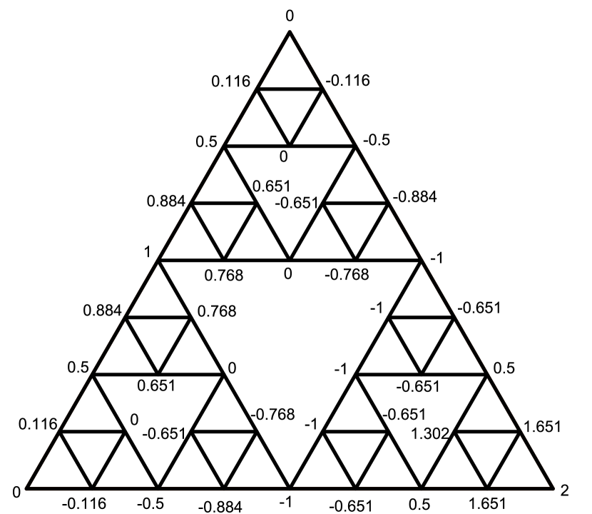
$\varphi_{4}$

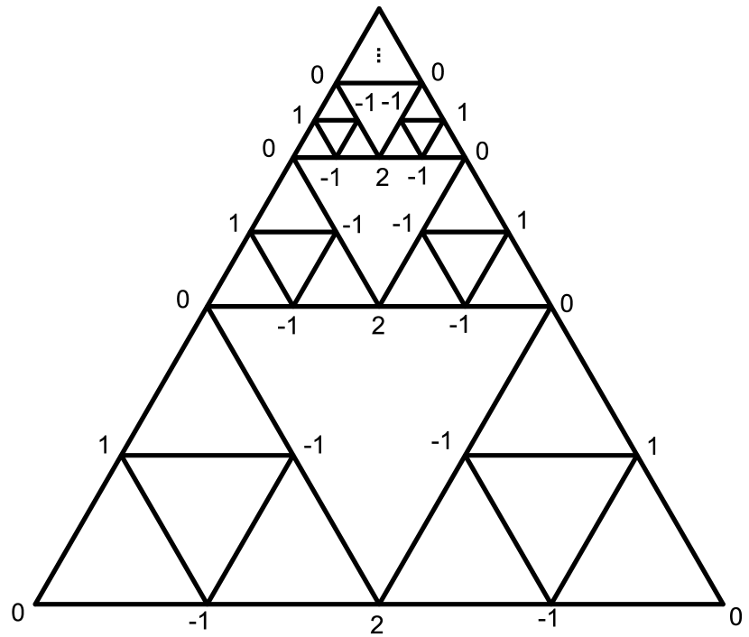
$f$

Figure 5.1. Functions in Example 9

6. Wave Kernel And Heat Kernel Upper Bound

Since the wave solution has infinite propagation speed for some fractals, we would like to get off-diagonal estimates of the solution of the wave equation for those fractals.

We define $P_{t}u$ be the heat solution with initial data $u$ after time $t$ where $t>0$, that is,

$$P_{t}(\sum a_{n}\varphi_{n})=\sum a_{n}e^{-\lambda_{n}t}\varphi_{n}$$

where $u=\sum a_{n}\varphi_{n}$. Also, define $W_{t}u$ to be the solution of the wave equation with initial data $u$ and initial velocity $0$ after time $t$ where $t>0$, that is,

$$W_{t}(\sum a_{n}\varphi_{n})=\sum a_{n}\cos(\sqrt{\lambda_{n}}t)\varphi_{n}.$$

In this section, we assume the heat equation satisfies the following kernel upper bound:

(6.1) $$p(x,y,t)\leq\frac{C}{t^{\alpha}}\exp\left(-C\left(\frac{d(x,y)^{\beta}}{t}\right)^{1/(\beta-1)}\right)$$

for some $\alpha$ and some $\beta>2$ which is true for many fractals [8, 7].

Lemma 10.

Assume the heat kernel satisfies the upper bound (6.1). For $f\in L^{1}(K)$, we have

$$|P_{t+1/z}f(x)|\leq\frac{C}{t^{\alpha}}\exp\left(-Cr^{\frac{\beta}{\beta-1}}z^{\frac{2-\beta}{\beta-1}}\text{Re}z\right)||f||_{1}$$

for $t>0$ where $r=d(x,\text{supp}f)$.

Proof.

By scaling $f$, we may assume $||f||_{1}=1$. Let $u(z)=P_{t+1/z}f(x)$ which is analytic on $\{{\rm Re}z>0\}$. Note that

$$p(x,y,z) = \sum e^{-\lambda_{n}z}\varphi_{n}(x)\varphi_{n}(y)$$

$$\leq \left(\sum e^{-\lambda_{n}\text{Re}z}\varphi_{n}^{2}(x)\right)^{1/2}\left(\sum e^{-\lambda_{n}\text{Re}z}\varphi_{n}^{2}(x)\right)^{1/2}$$

$$\leq \frac{C_{1}}{(\text{Re}z)^{\alpha}}.$$

Therefore, we have $|u(z)|\leq\frac{C}{t^{\alpha}}$. On the other hand, the kernel upper bound tells us that

$$|u(z)|\leq\frac{C}{t^{\alpha}}\exp\left(-Cr^{\frac{\beta}{\beta-1}}z^{\frac{1}{\beta-1}}\right).$$

Because of symmetry, we only prove the statement for the first quadrant. Consider the strip $\Omega=\{x+iy:\ 0<y<\frac{\pi}{2}\}$ and let

$$v(z)=u(\exp(z)).$$

By assumption, $|v(z)|\leq\frac{C}{t^{\alpha}}$ for $z\in\overline{\Omega}$ and $|v(x)|\leq\frac{C}{t^{\alpha}}\exp(-C\exp(\alpha x))$ for $x\in\mathbb{R}$. Let

$$f(z)=\frac{v(z)}{\frac{C}{t^{\alpha}}\exp(-Cr^{\frac{\beta}{\beta-1}}\exp(\frac{1}{\beta-1}z))}.$$

Now $f$ is analytic on the strip $\Omega$, continuous on $\overline{\Omega}$ and bounded by $1$ on boundary of $\Omega$. Also, it satisfies a decay estimate

$$|f(z)|\leq\exp(Cr^{\frac{\beta}{\beta-1}}\exp(\frac{1}{\beta-1}|z|))\quad(z\in\Omega).$$

By the Phragmén-Lindelöf theorem, we have $|f|\leq 1$ on $\Omega$. Thus, for $z\in\{\text{Re}z>0\}$, we have

$$|u(z)| \leq \frac{C}{t^{\alpha}}|\exp(-Cr^{\frac{\beta}{\beta-1}}z^{\frac{1}{\beta-1}})|$$

$$\leq \frac{C}{t^{\alpha}}\exp\left(-Cr^{\frac{\beta}{\beta-1}}z^{\frac{1}{\beta-1}}\sin(\frac{\pi}{2}-|\mbox{arg}z|)\right)$$

$$\leq \frac{C}{t^{\alpha}}\exp\left(-Cr^{\frac{\beta}{\beta-1}}z^{\frac{2-\beta}{\beta-1}}\text{Re}z\right)$$

∎

Recall that the heat equation is the averaged wave equation and we can use this to recover the lower frequency of the solution of wave equation. Therefore, mollified solutions is exponentially small outside the support of initial function when time is small.

Lemma 11.

For $\frac{1}{4t}\geq\gamma>0$ and$-1<\alpha<0$, we have

$$\min_{\text{Re}(z)=\gamma}\left|\frac{1}{z^{-1}+t}\right|^{\alpha}\text{Re}(\frac{1}{z^{-1}+t})\geq C_{\alpha}t^{-\alpha/2}\gamma^{1+\alpha/2}$$

where $C_{\alpha}$ is a constant depends on $\alpha$ only.

Proof.

We may assume $\arg(\frac{1}{z^{-1}+t})\geq 0$ because of symmetry. For $0\leq\arg(\frac{1}{z^{-1}+t})\leq\frac{\pi}{4}$, we have

$$\left|\frac{1}{z^{-1}+t}\right|^{\alpha}\text{Re}(\frac{1}{z^{-1}+t}) \geq \frac{1}{\sqrt{2}}\left|\frac{1}{z^{-1}+t}\right|^{\alpha+1}$$

$$\geq \frac{1}{\sqrt{2}}\left|\frac{1}{\gamma^{-1}+t}\right|^{\alpha+1}$$

For $\arg(\frac{1}{z^{-1}+t})>\frac{\pi}{4}$, let $z=\gamma+ix$. We have

$$\frac{1}{z^{-1}+t}=\frac{\gamma^{2}+x^{2}}{(t(\gamma^{2}+x^{2})+\gamma)^{2}+x^{2}}(t(\gamma^{2}+x^{2})+\gamma+ix).$$

Since $\arg(\frac{1}{z^{-1}+t})>\frac{\pi}{4}$, we have $x>t(\gamma^{2}+x^{2})+\gamma$. Hence,

$$\frac{\gamma^{2}+x^{2}}{(t(\gamma^{2}+x^{2})+\gamma)^{2}+x^{2}}\geq\frac{1}{2}.$$

Therefore,

$$\left|\frac{1}{z^{-1}+t}\right|^{\alpha}\text{Re}(\frac{1}{z^{-1}+t}) \geq \left(\frac{1}{2}\right)^{\alpha+1}((t(\gamma^{2}+x^{2})+\gamma)^{2}+x^{2})^{\alpha/2}(t(\gamma^{2}+x^{2})+\gamma)$$

$$\geq \left(\frac{1}{2}\right)^{\alpha+1}x^{\alpha}(tx^{2}+\gamma)$$

$$\geq \left(\frac{1}{2}\right)^{\alpha+1}\left(\sqrt{\frac{-\alpha}{2+\alpha}}\right)^{\alpha}\frac{\gamma^{\alpha/2}}{t^{\alpha/2}}(\frac{2}{2+\alpha}\gamma)$$

where the last line comes from minimizing $x$ over $x\geq 0$. Combining the two cases, we get

$$\min_{\text{Re}(z)=\gamma}\left|\frac{1}{z^{-1}+t}\right|^{\alpha}\text{Re}(\frac{1}{z^{-1}+t}) \geq C_{\alpha}\min(\left|\frac{1}{\gamma^{-1}+t}\right|^{\alpha+1},\gamma^{1+\alpha/2}t^{-\alpha/2})$$

$$\geq C_{\alpha}t^{-\alpha/2}\min(t^{-1},\gamma)^{1+\alpha/2}$$

∎

Theorem 12.

Assume the heat kernel satisfies the upper bound (6.1). Let $\phi_{\sigma}(t)=\frac{1}{\sqrt{2\pi\sigma}}\exp(-\frac{t^{2}}{2\sigma})$. For $\sigma=O\left(\left(\frac{t^{\beta-1}}{r^{\beta}}\right)^{\frac{1}{\beta-2}}\right)$ and $f\in L^{1}$, we have

$$|(\phi_{\sigma}*Wf)(x,t)|\leq\frac{C}{t^{\alpha+1+\frac{5\beta-5}{\beta-2}}r^{\frac{5\beta}{\beta-2}}\sigma^{5/2}}\exp(-C\left(\frac{r^{2}}{t}\right)^{\frac{\beta}{\beta-2}}\sigma)||f||_{1}$$

where $r=\text{d}(x,\text{supp}f)$. Furthermore, for $\sigma=O\left(\left(\frac{t^{2\beta-2}}{r^{2\beta}}\right)^{\frac{1}{\beta-2}}\right)$ and $P_{-\sigma}f\in L^{1}$ , we have

$$|Wf(x,t)|\leq\frac{C}{t^{\alpha+1+\frac{5\beta-5}{\beta-2}}r^{\frac{5\beta}{\beta-2}}\sigma^{5/2}}\exp(-C\left(\frac{r^{2}}{t}\right)^{\frac{\beta}{\beta-2}}\sigma)||P_{-\sigma}f||_{1}$$

where $r=\text{d}(x,\text{supp}f)$.

Proof.

The relation between heat and wave equation can be written as

$$\exp(-s\lambda_{n})=\sqrt{\frac{1}{4\pi s}}\int_{-\infty}^{\infty}\cos(t\sqrt{\lambda_{n}})e^{-\frac{t^{2}}{4s}}dt.$$

Changing some variables, we get

$$\sqrt{\frac{\pi}{s}}\exp\left(-\frac{\lambda_{n}}{4s}\right)=\int_{0}^{\infty}\frac{1}{\sqrt{t}}\cos(\sqrt{\lambda_{n}t})e^{-st}dt.$$

The inverse Laplace transform implies

$$\frac{1}{\sqrt{t}}\cos(\sqrt{\lambda_{n}t}) = \frac{1}{2\pi i}\int_{\gamma-i\infty}^{\gamma+i\infty}\sqrt{\frac{\pi}{s}}\exp\left(-\frac{\lambda_{n}}{4s}+st\right)ds.$$

for any $\gamma>0$. The mollified cosine is

$$\left(\phi*\cos(\sqrt{\lambda_{n}}\cdot)\right)(t) = e^{-\frac{\sigma}{2}\lambda_{n}}\cos(\sqrt{\lambda_{n}}t)$$

$$= \frac{t}{2\pi i}\int_{\gamma-i\infty}^{\gamma+i\infty}\sqrt{\frac{\pi}{s}}\exp\left(-\lambda_{n}(\frac{1}{4s}+\frac{\sigma}{2})+st^{2}\right)ds.$$

Hence, the mollified solution can be computed as

$$(\phi_{\sigma}*Wf)(t)=\frac{t}{2\pi i}\int_{\gamma-i\infty}^{\gamma+i\infty}\sqrt{\frac{\pi}{s}}e^{st^{2}}P_{(4s)^{-1}+\frac{\sigma}{2}}fds.$$

Rewrite the equation by letting $u(z)=P_{(4z)^{-1}+\frac{\sigma}{4}}f$ and $v(t)=(\phi_{\sigma}*Wf)(t)$, we have

(6.2) $$v(t) = \frac{t}{2\sqrt{\pi}i}\int_{\gamma-i\infty}^{\gamma+i\infty}s^{-1/2}e^{st^{2}}u(\frac{1}{s^{-1}+\sigma})ds$$

$$= \frac{1}{4\sqrt{\pi}it}\int_{\gamma-i\infty}^{\gamma+i\infty}s^{-3/2}e^{st^{2}}u(\frac{1}{s^{-1}+\sigma})ds+$$

$$\frac{-\sqrt{\pi}}{2\pi it}\int_{\gamma-i\infty}^{\gamma+i\infty}s^{-1/2}e^{st^{2}}u^{\prime}(\frac{1}{s^{-1}+\sigma})\frac{1}{(\frac{1}{s}+\sigma)^{2}}\frac{1}{s^{2}}ds.$$

Using Lemma 10, we have

$$|u(\frac{1}{s^{-1}+\sigma})| \leq \frac{C}{t^{\alpha}}\exp\left(-Cr^{\frac{\beta}{\beta-1}}\left|\frac{1}{s^{-1}+\sigma}\right|^{\frac{2-\beta}{\beta-1}}\text{Re}\frac{1}{s^{-1}+\sigma}\right)||f||_{1}.$$

Using Lemma 11, for $\frac{1}{\sigma}>4\gamma>0$ , we have

$$|u(\frac{1}{s^{-1}+\sigma})| \leq \frac{C}{t^{\alpha}}\exp\left(-Cr^{\frac{\beta}{\beta-1}}\gamma^{\frac{\beta}{2\beta-2}}\sigma^{\frac{\beta-2}{2\beta-2}}\right)||f||_{1}$$

for $\text{Re}s=\gamma$. By the Cauchy integral formula, we have

$$|u^{\prime}(\frac{1}{s^{-1}+\sigma})| \leq \frac{C|s^{-1}+\sigma|}{t^{\alpha}}\exp\left(-Cr^{\frac{\beta}{\beta-1}}\gamma^{\frac{\beta}{2\beta-2}}\sigma^{\frac{\beta-2}{2\beta-2}}\right)||f||_{1}$$

$$\leq \frac{C}{t^{\alpha}\gamma}\exp\left(-Cr^{\frac{\beta}{\beta-1}}\gamma^{\frac{\beta}{2\beta-2}}\sigma^{\frac{\beta-2}{2\beta-2}}\right)||f||_{1}$$

for $\text{Re}s=\gamma$. Substituting in (6.2), we get

$$|v(t)| \leq \frac{Ce^{\gamma t}}{t^{\alpha+1}}(\int_{0}^{\infty}|\gamma+is|^{-3/2}ds+\frac{1}{\gamma}\int_{0}^{\infty}|\gamma+is|^{-5/2}ds)\exp(-Cr^{\frac{\beta}{\beta-1}}\gamma^{\frac{\beta}{2\beta-2}}\sigma^{\frac{\beta-2}{2\beta-2}})$$

$$\leq \frac{Ce^{\gamma t}}{t^{\alpha+1}}(\frac{1}{\sqrt{\gamma}}+\frac{1}{\gamma^{5/2}})\exp(-Cr^{\frac{\beta}{\beta-1}}\gamma^{\frac{\beta}{2\beta-2}}\sigma^{\frac{\beta-2}{2\beta-2}})$$

The first result follows from putting $\gamma=\frac{\left(\frac{\beta}{2\beta-2}\right)^{\frac{\beta-2}{2\beta-2}}r^{\frac{2\beta}{\beta-2}}\sigma}{t^{\frac{2\beta-2}{\beta-2}}}$. The second result follows from the identity

$$\left(\phi*\cos(\sqrt{\lambda_{n}}\cdot)\right)(t)=e^{-\frac{\sigma}{2}\lambda_{n}}\cos(\sqrt{\lambda_{n}}t).$$

∎

7. Acknowledgment

I would like to thank the Department of Mathematics in the Chinese University of Hong Kong and Cornell University providing me supports and chance to do research via joining in the Research Experiences for Undergraduates Program. I am grateful to Prof Robert Strichartz for his valuable discussions and suggestions. Also, he read the original manuscript and suggested several improvements. Lastly, I would like to thank Ms. Mavis Chan for her valuable suggestions.