Memristive excitable cellular automata
Abstract
The memristor is a device whose resistance changes depending on the polarity and magnitude of a voltage applied to the device’s terminals. We design a minimalistic model of a regular network of memristors using structurally-dynamic cellular automata. Each cell gets info about states of its closest neighbours via incoming links. A link can be one ’conductive’ or ’non-conductive’ states. States of every link are updated depending on states of cells the link connects. Every cell of a memristive automaton takes three states: resting, excited (analog of positive polarity) and refractory (analog of negative polarity). A cell updates its state depending on states of its closest neighbours which are connected to the cell via ’conductive’ links. We study behaviour of memristive automata in response to point-wise and spatially extended perturbations, structure of localised excitations coupled with topological defects, interfacial mobile excitations and growth of information pathways.
Keywords: memristor, cellular automaton, excitable medium
1 Introduction
The memristor (a passive resistor with memory) is a device whose resistance changes depending on the polarity and magnitude of a voltage applied to the device’s terminals and the duration of this voltage’s application. Its existence was theoretically postulated by Leon Chua in 1971 based on symmetry in integral variations of Ohm s laws [4, 5, 6]. The memristor is characterised by a non-linear relationship between the charge and the flux; this relationship can be generalised to any two-terminal device in which resistance depends on the internal state of the system [5]. The memristor cannot be implemented using the three other passive circuit elements — resistor, capacitor and inductor therefore the memristor is an atomic element of electronic circuitry [4, 5, 6]. Using memristors one can achieve circuit functionalities that it is not possible to establish with resistors, capacitors and inductors, therefore the memristor is of great pragmatic usefulness. The first experimental prototypes of memristors are reported in [19, 7, 20]. Potential unique applications of memristors are in spintronic devices, ultra-dense information storage, neuromorphic circuits, and programmable electronics [17].
Despite explosive growth of results in memristor studies there is still a few (if any) findings on phenomenology of spatially extended non-linear media with hundreds of thousands of locally connected memristors. We attempt to fill the gap and develop a minimalistic model of a discrete memristive medium. Structurally-dynamic (also called topological) cellular automata [11], [8] seem to be an ideal substrate to imitate discrete memristive medium. A cellular automaton is structurally-dynamic when links between cells can be removed and reinstated depending on states of cells these links connect. Strcturally-dynamic automata are now proven tools to simulate physical and chemical discrete spaces [16, 9, 10, 15, 3] and graph-rewriting media [18]; see overview in [12].
We must highlight that simulation of cellular automata in networks of memristors is discussed in full details in [13]. Itoh-Chua memristor cellular automata are automata made of memristors. Memristive cellular automata studied in present paper are cellular automata which exhibit, or rather roughly imitate, certain memristive properties but otherwise are classical excitable structurally-dynamic cellular automata.
The paper is structured as follows. Memristive automata are defined in Sect. 2. In Sect. 3 we analyse space-time dynamics of the automata in response to external perturbations. Anatomy of stationary oscillating localizations is presented in Sect. 4. We analyse structure of disordered excitation worms propagating at the boundary between disorganised and ordered link domains in Sect. 5. Collision-based approach to layout of conductive pathways is given in Sect. 6. Some ideas of further studies are outlined in Sect. 7.
2 Memristive automaton
Definition 1
A memristive automaton is a structurally-dynamic excitable cellular automaton where a link connecting two cells is removed or added if one of the cells is in excited state and another cell is in refractory state.
A cellular automaton is an orthogonal array of uniform finite-state machines, or cells. Each cell takes finite number of states and updates its states in discrete time depending on states of its closest neighbours. All cells update their states simultaneously by the same rule. We consider eight-cell neighbourhood and three cell-states: resting , excited , and refractory . Let be a neighbourhood of cell . A cell has a set of incoming links which take states and . A link is a link of excitation transfer from cell to cell . A link in state is considered to be high-resistant, or non-conductive, and link in state low resistant, or conductive. A link-state is updated depending on states of cells and at time step : . Resting state gives little indication of cell’s previous history, therefore we will consider not resting cells contributing to a link state updates. When cells and are in the same state (bother cells are in state or both are in state ) no ’current’ can flow between the cells, therefore scenarios are not taken into account. Thus we assume that the only situations when and may lead to changes in links conductivity:
| (1) |
where and . Thus we consider two types of automata : and .
A resting cell excites ( transition) depending on number of excited neighbours.
There are two ways to calculate a weighted sum of number of excited neighbours:
-
1.
-
2.
,
where if and otherwise.
Thus, we consider two types of memristive automata. In automaton a resting cell excites if . In automaton a resting cell excites if or .
Note 1
A polarity of a current is imitated by excitable cellular automaton using exctited and refractory states. If a cell is in state and a cell is in state then cell symbolises an anode, and cell a cathode. And we can say that a current flows from to . Indeed, such an abstraction is at the edge of physical reality, however this is the only way to develop a minimal discrete model of a memristive network. In automaton the condition symbolises propagation of a high intensity current along all links, including links non-conductive for a low intensity current. This high intensity current in resets conductivity of the links and also states of cells. The condition reflects propagation of a low intensity current along conductive links. The current of low intensity does not affect states of links but only states of cells.
2.1 Experiments
We experiment with cell automaton arrays, with non-periodic absorbing boundaries. We conduct experiments for two initial conditions on links’ ’conductivity’ —
-
•
-condition: all links are conductive (for every cell and its neighbour ), and
-
•
-condition: all links are non-conductive (for every cell and its neighbour ).
While testing automata’s response to external excitation we use point-wise and spatially extended stimulations. By point-wise stimulation we mean excitation of a single cell () or a couple of cells () of resting automata. These are minimal excitations to start propagating activity.
Let -disc be a set of cells which lie at distance not more than from the array centre , . When undertaking -stimulation we assign excited state to a cell of with probability 0.05. In some cases we apply -stimulation twice as follows. An automaton starts in - or -condition, we apply -stimulation first time (we call it -excitation) and wait till excitation waves propagate beyond boundaries of the array or a quasi-stationary structure is formed. After this transient period we apply -stimulation again (-excitation) without resetting links states.
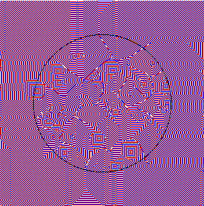
Space-time dynamics of automata is illustrated by configurations of excitations and dynamics of link conductivity is shown either explicitly by arrows (in small configuration) or via grey-scale representation of cells’ in-degrees: cell is represented by pixel with grey-value . Despite not representing exact configuration of local links, in-degrees give us a rough indicator of spatial distribution of conductivity in the medium. The higher is the in-degree at a given point, the higher is the conductivity at this point.
3 Phenomenology
Finding 1
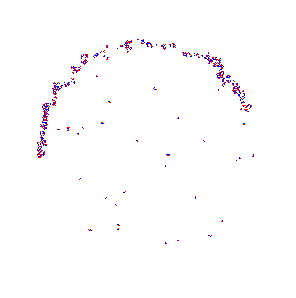
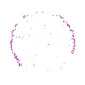
A point-wise stimulation of automaton leads to a persistent excitation, while automaton returns to a resting state.


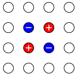
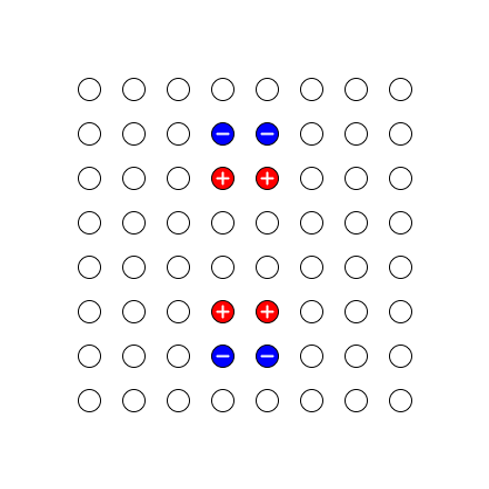
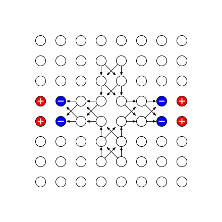
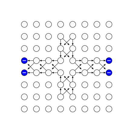
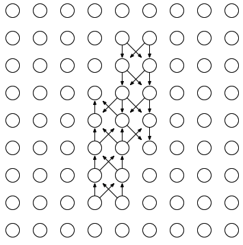
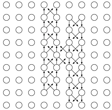
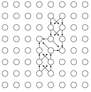
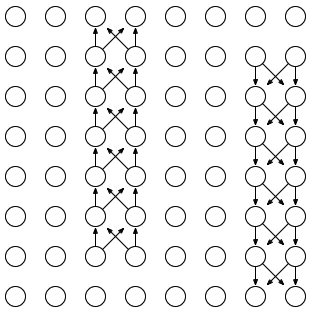
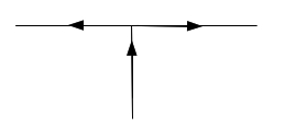
A single-cell excitation of resting automaton (Fig. 1) or two-cell excitation of resting automaton (Fig. 2) in initial conditions lead to formation of a ’classical’ excitation wave-front. The wave-front propagates omni-directionally away from the initial perturbation site and updates states of links it is passing through.
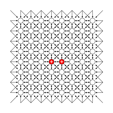
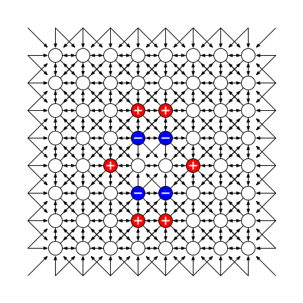
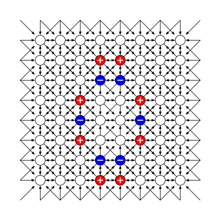
Links leading from cells to the neighbours they excited are made non-conductive in development of (Figs. 1 and 2); or we can say that links corresponding to normal vectors of propagating wave-front are made non-conductive. Cell excited at time step becomes isolated. The situation is similar in development of automata and with the only difference that links connecting cells which are excited at time step to cells they have been excited by are removed.
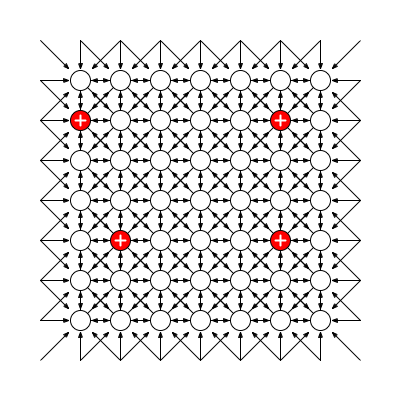
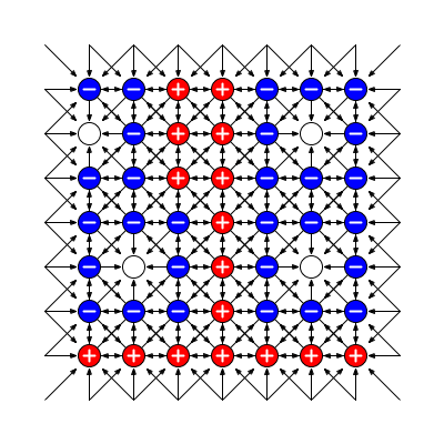
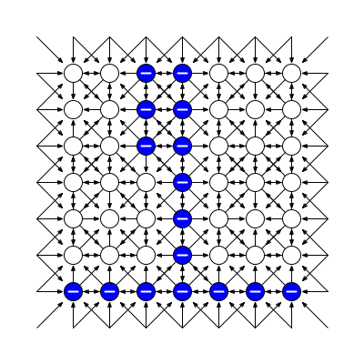
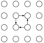
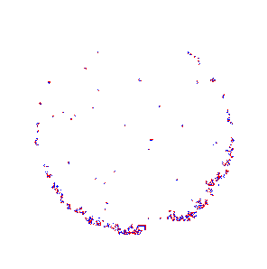
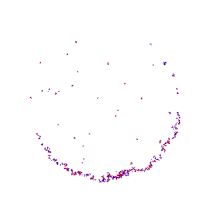
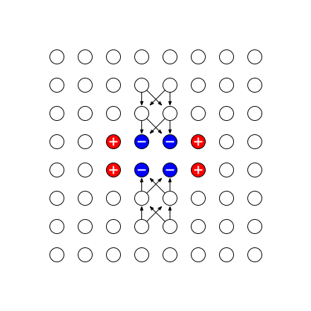
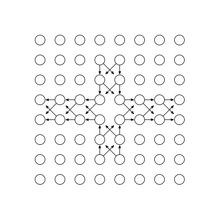
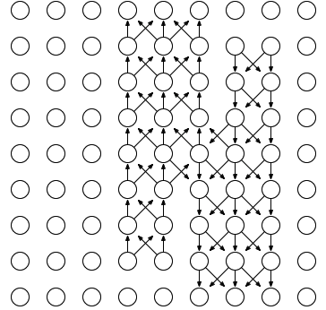
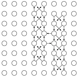
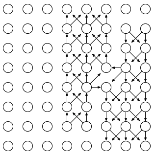
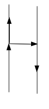
In summary, in automata links associated with forward propagation of perturbation are made non-conductive, and in links associated with backward propagation are made non-conductive. Excitation wave-front travelling from a single stimulation site forms a domain of co-aligned links. Excitation waves initiated in different cells collide and merge. Boundaries between domains formed by different fronts are represented by distinctive configurations of links (Fig. 3).
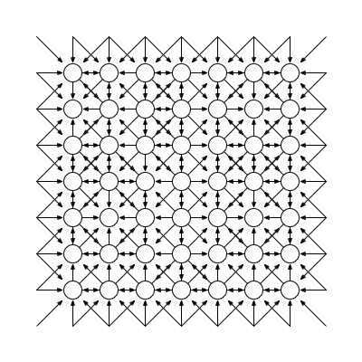
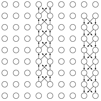
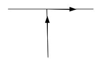
Automaton is non-excitable in -conditions because no excitation can propagate along non-conductive links. An outcome of two-site excitation of resting automaton in -condition depends on configuration of the initial excitation.
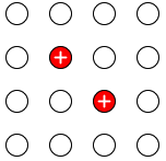
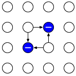
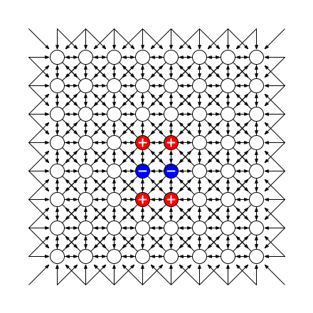
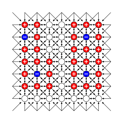
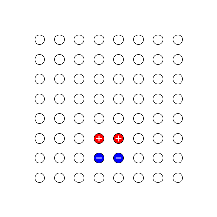
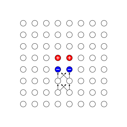
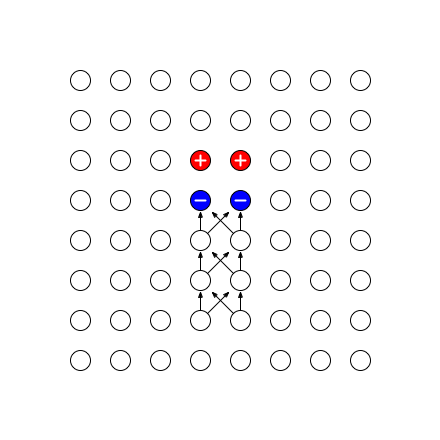
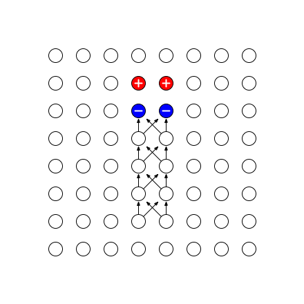
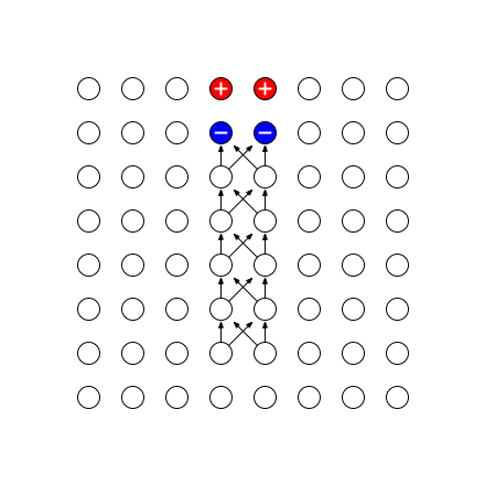
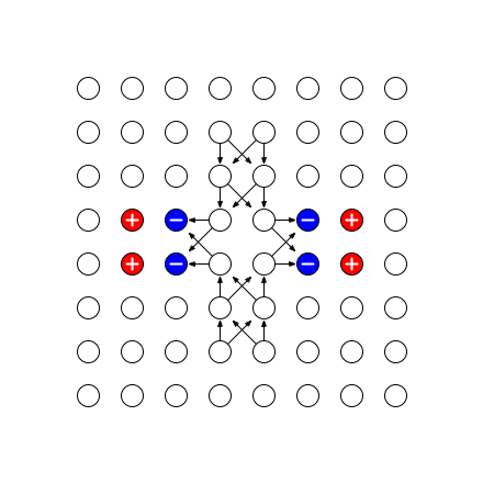
Let two diagonal neighbours (north-west and south-east) be excited (Fig. 4a) at time step . These two cells transfer excitation to their two neighbours (north-east and south-west) as shown in Fig. 4b. Only links from north-west cell to north-east and south-west, and south-east to south-west and north-east are formed (Fig. 4c) and excitation becomes extinguished (Fig. 4d).


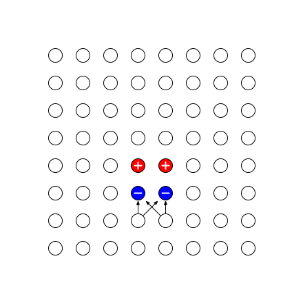
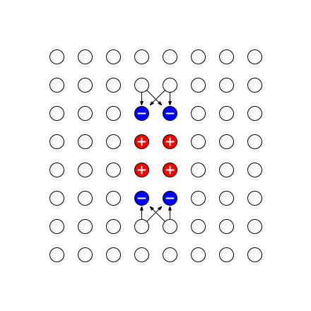
Let excited cells be neighbours at the same row of cells (Fig. 5a). If they are excited at time step then their north and south neighbours are excited due to condition taking place (Fig. 5b). The localised (two-cell size) excitations propagate north and south (Fig. 5c) and make links pointing backwards (towards source of initial excitation) conductive. At the second iteration cell lying east and west of initially perturbed cells becomes excited (Fig. 5c). By that initially perturbed cells return to resting state (Fig. 5d) and thus they become excited again. A growing pattern of recurrent excitation fills the lattice (Fig. 5de).
Finding 2
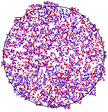
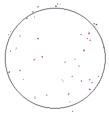
Repeated stimulation of memristive automata in a spatially-extended domain leads to formation of either disorganised activity domain emitting target waves of excitation or a sparse configuration of stationary oscillating localizations.
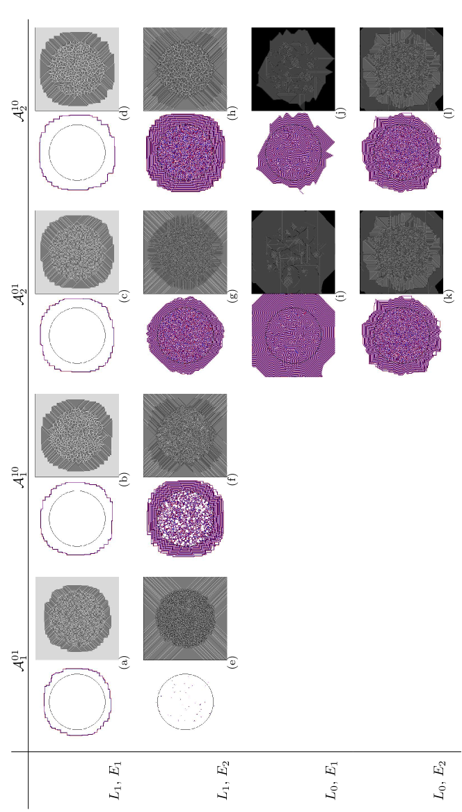
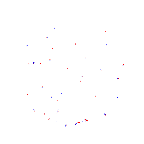
Examples of excitation dynamics in response to - and -excitations are shown in Fig. 6. Each singular perturbation in the first stimulation of automata being in -condition leads to propagation of excitation. The waves merge into a single wave and disappear beyond lattice boundary. Merging of waves outside into a single wave is reflected in cells’ in-degree distribution in Fig. 19.
Automata’ behaviour become different after second -stimulation (-excitation). They all exhibit quasi-chaotic dynamic inside boundaries of disc (shown by circle in Fig. 6); cell in-degrees’ distributions of the automata are similar (Fig. 18). However the excitation dynamics in automaton is reduced (after long transient period) to stationary oscillating localizations while in automata , , and excitations outside boundaries of initial stimulation merge into target waves (Fig. 6 and Fig. 19). Oscillating localizations developed in stay inside the boundaries of .
Random excitation is extinguished immediately in automata being in -condition of total non-conductivity. When automaton in -condition is excited, the quasi-random excitation activity persists inside boundaries of while omni-directional waves are formed outside . Patterns of activity are not changed significantly after second random perturbation, -excitation (Fig. 6).
If there are both excited and refractory states in the external stimulation domain the developments are almost the same but and shows persistent excitation activity already at the first stimulation.
4 Oscillating localisations
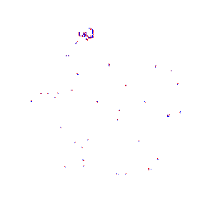
Finding 3
-excitation of leads to formation of excitation wave-fragments trapped in a structurally defined domains.
| Characteristic | ||
|---|---|---|
| Period | 12 | 26 |
| Minimum mass | 2 | 2 |
| Maximum mass | 7 | 7 |
| Minimum size | 2 | 2 |
| Maximum size | 36 | 9 |
| Minimum density | 1 | 1 |
| Maximum density |
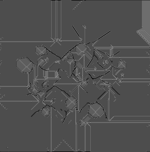
-excitation of leads to formation of sparsely distributed localised oscillating excitations, or oscillators (Fig. 7). An oscillating localisation (oscillator) usually consist of one or two mobile localizations which shuffle inside a small compact domain of the automaton array. This micro-wave is updating states of links and thus influencing its own behaviour. , after -stimulation and formation of oscillating localizations, is characterised by a smooth balanced distribution of cells in-degrees (Fig. 18, table entry , ).
Examples of two most commonly found oscillators — and — are shown in Figs. 8 and 9, and their characteristics in Fig. 10. Both oscillators have exactly the same minimum and maximum masses (measured as a sum of cells in excited and refractory states). Oscillator has much longer period than and larger maximum density. Oscillator spans large space during its transformation cycle, it occupies a sub-array of cells when in its largest form.
In its minimal form consists of two cells: one cell is in state another in state (Fig. 8, ). At next two steps of ’s transformations a small localised excitation is formed. It propagates north (Fig. 8, ). At fourth step of oscillator ’s transformation the travelling localised excitation splits into two excitations: one travels north-west, another south (Fig. 8, ). The localisation travelling south returns to exact position of the first step excitation, just with swapped excited and refractory states (Fig. 8, compare with ) and then repeats a cycle of transformations (compare with an with ). The excitation travelling north-west become extinguished ().
A couple is a minimal configuration of oscillator (Fig. 9, ). When the localisation starts it is development in configuration , and configuration of links’ conductivity as shown in Fig. 9, it is transformed into excitation wave-fragment propagating east and north-east (Fig. 9, ). At fourth step of oscillator’s transformation the wave-fragment shrinks and by step the oscillator repeats its original state yet rotated by clockwise. New excitation wave-fragment emerges and propagates west and south-west (Fig. 9, ). The fragment contracts to configuration by step . Then development and transformation of excitation wave-fragments is repeated (Fig. 9, ). The localisation returns to its original configuration at .
Most oscillating localizations observed in experiments with have very long periods. This is because the oscillators’ behaviour is determined not only by cell-state transitions rules, as in classical cellular automata, but also by topology of links modified by repeated random stimulation and dynamics of the links affected by oscillators themselves.
5 Dynamics of excitation on interfaces
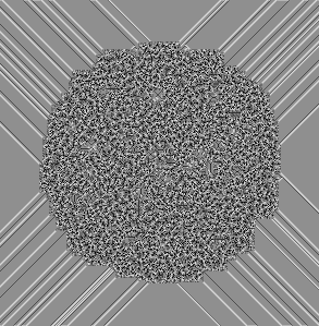
Finding 4
Automaton exhibits localizations propagating along the boundary of disordered and ordered conductivity domains.
As previously discussed, after -excitation of the automaton becomes separated into two domains. One domain has a disorganised appearance, it lies inside boundaries of . This domain is characterised by quasi-random discoidal configuration of cell in-degrees (Fig. 7c). Second domain, cells lying outside , represents ordered configurations of links (Fig. 7c). The links are co-alined during target wave propagation outward . See Figs. 18 and 19 for distribution of cell in-degrees in disordered and ordered domaines.
In automaton a link from cell to cell becomes non-conductive at time step if and . Thus target waves travel ouside of form non-conductive pathways. If we stimulate automaton in these domains of ordered links no distal propagation of excitation will be observed, however, a worm of disordered excitations is formed at the boundary between disordered and ordered configurations of links.
When configuration of oscillating localizations becomes stationary (in a sense that the localizations do not travel outside their fixed domains) we apply a few-cells wide excitation at the boundary of (Fig. 11a), north-north-west localised excitation, which exceeds in size existing oscillating localizations). An extended cluster, or a worm (a group of excited and refractory states with a preferable direction of growth), of excited and refractory cells is formed (Fig. 11b). It expands along the boundary between domains. Two heads of the emerging worm — one head moves clockwise and another anticlockwise — are clearly visible in (Fig. 11). At some point the worm undergoes sub-division (Fig. 11c) and it breaks into two independent worms (Fig. 11d). Each new worm has an extended head and gradually thinning tail. Thickness of a worm, measured in a number of non-resting cells along the worm body, is shown in Fig. 12.
6 Building conductive pathways
Finding 5
By exploring collisions between excitation wave-fragments travelling in one can built information transmission pathways in an initially non-conductive medium. Routing primitives realised include signal splitting, signal echoing and signal turning.
Localizations travelling in , -condition, can form pathways conductive for low-strength excitations. For example, a localisation of two excited and two refractory states propagates in in the direction of its excited ’head’. The localisation forms a chain of conductive links oriented opposite to the localisation’s velocity vector in case of , and in the direction of the localisation’s propagation in case of (Fig. 13).
| 0 | 1 | 2 | 3 | 4 | |
|---|---|---|---|---|---|
| odd | 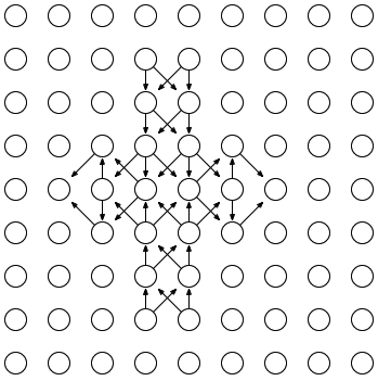 |
 |
 |
 |
 |
| even | 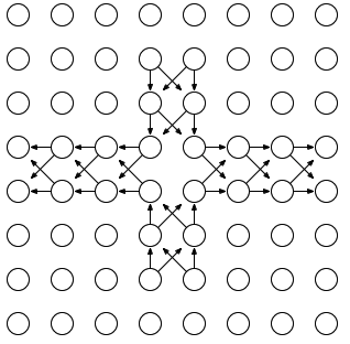 |
 |
 |
 |
 |
A layout of conductive pathways, or ’wires’, is determined by outcomes of collisions between path-laying particles. A detailed example of such collision-determined pathway building is shown in Fig. 14. Two travelling localizations, -particles111-particles are localizations consisting of two excited and two refractory states, which move along rows or columns of an excitable cellular array [2], are initiated in facing each other with their excited heads (Fig. 14a). One particle propagates south another north (Fig. 14a). When the particles collide they undergo elastic-like collision, in the result of which two -particles are formed: one travels east another west (Fig. 14c–f). When a weak excitation rule — a cell is excited if at least one neighbour is excited and no links are updated — is imposed on the automaton the pathways formed by these two colliding particles becomes selective. If an excitation is initiated in the southern or northern channel the excitation propagates till cross-junction and then branches into eastern and northern channels.
Pathways built by two -particles undergoing head-on collision being in different phases (odd and even distance between their start positions) and lateral offsets are shown in Fig. 15. Most T-bone collisions between -particles lead to formation of omni-directionaly growing excitation patterns. Only in situations when one particle hits a tail of another particle no uncontrollable growth occurs. The particle hitting a tail of another particle extinguishes and the other particle continues its journey undisturbed.
There are primitives of information routing implementable in collisions between -particles (Fig. 16). T-branching, or signal splitting, (Fig. 16a) is built by particles colliding with zero lateral shift and even number of cells between their initial positions (e.g. Fig. 15, entry (even, 0)). When signal travelling north reaches cross-junctions it splits into two signals – one travel west and another travels east; no signal continues straight propagation across junction.
Echo primitive (Fig. 16b) is constructed in a head-on collision between -particles with lateral shift two or three cells (see (e.g. Fig. 15, entries (odd, 2), (odd, 3), (even, 2), (even, 3)). The echo primitive consists of two anti-aligned (e.g. one propagates information northward and another southward) parallel information pathways. There is a bridge between the pathways. When signal propagating along one pathway reaches the bridge, it splits, daughter signal enters second pathway and propagates in the direction of mother signal’s origination. In (Fig. 16b) mother-signal propagates north and daughter-signal south.
Turn primitive (Fig. 16c) is implemented in T-bone collision between two -particles. A signal generated at either of the pathways propagates in the direction of -particle which trajectory was undisturbed during collision.
7 Discussion
We designed a minimalistic model of a two-dimensional discrete memristive medium. Every site of such medium takes triple states, and a binary conductivity of links is updated depending on states of sites the links connect. The model is a hybrid between classical excitable cellular automata [14] and classical structurally-dynamic cellular automata [11]. A memristive automaton with binary cell-states would give us even more elegant model however by using binary cell-states we could not easily detect source and sink of simulated ’currents’. Excitable cellular automata provide us with all necessary tools to imitate current polarity and to control local conductivity. From topology of excitation wave-fronts and wave-fragments we can even reconstruct relative location of a source of initiated current.
We defined two type of memristive cellular automata and characterised their space-time dynamics in response to point-wise and spatially extended perturbations. We classified several regimes of automata excitation activity, and provided detailed accounts of most common types of oscillating localizations. We did not undertake any systematic search for minimal oscillators though but just exemplified two most commonly found after random spatially-extended stimulation. Exhaustive search for all possible localised oscillations could be a topic of further studies.
With regards to formation of conductive pathways just few possible versions amongst many implementable were discussed in the papers. Opportunities to grow ’wires’ in memristive automata are virtually unlimited. For example, in , -start, after first -stimulation (Fig. 17) generators of spiral and target waves are formed inside . Boundaries between the generators (they provide a partial approximation of a discrete Voronoi diagram over centres of the generators) are comprised of cells with high in-degrees. Such chains of high in-degree cells can play a role of conductive pathways even if we increase excitation threshold of the medium.
References
- [1] Adamatzky A. Controllable transmission of information in excitable medium: the medium. Advanced Materials for Optics and Electronics 5 (1995) 145 -155.
- [2] Adamatzky A. Computing in Nonlinear Media and Automata Collectives (IoP, 2011).
- [3] R. Alonso-Sanz A structurally dynamic cellular automaton with memory, Chaos, Solitons and Fractals 32 (2006) 1285 -1295.
- [4] Chua L. O., Memristor — the missing circuit element. IEEE Trans. Circuit Theory 18 (1971) 507–519.
- [5] Chua L. O. and Kang S. M., Memristive devices and systems. Proc. IEEE 64 (1976) 209–223.
- [6] Chua L. O. Device modeling via non-linear circuit elements. IEEE Trans. Circuits Systems 27 (1980) 1014–1044.
- [7] Erokhin V., Fontana M.T. Electrochemically controlled polymeric device: a memristors (and more) found two years ago. (2008) arXiv:0807.0333v1 [cond-mat.soft]
- [8] Halpern P. and G. Caltagirone. Behavior of topological cellular automata. Complex Systems 4 (1990) 623 651.
- [9] Hasslacher B. and Meyer D. A. Modelling dynamical geometry with lattice gas automata. Int J Modern Physics C 9 (1998) 1597–1605.
- [10] Hillman D. Combinatorial spacetimes. (Ph.D. dissertation) 234 pp. arXiv:hep-th/9805066v1
- [11] Ilachinsky A. and Halpern P., Structurally dynamic cellular automata, Complex Systems 1 (1987) 503–527.
- [12] Ilachinsky A., Structurally Dynamic Cellular Automata Encyclopedia of Complexity and Systems Science 2009, Part 19, 8815–8850.
- [13] Itoh M. and Chua L. Memristor cellular automata and memristor discrete-time cellular neural networks. Int. J. Bifurcation and Chaos 19 (2009) 3605–3656.
- [14] Greenberg J. M. and Hastings S. P. Spatial patterns for discrete models of diffusion in excitable media, SIAM J. Appl. Math. 34 (1978) 515 -523.
- [15] Requardt M. A geometric renormalization group in discrete quantum space time. J. Math. Phys. 44 (2003) 5588.
- [16] Rosé H., Hempel H., Schimansky-Geier L. Stochastic dynamics of catalytic CO oxidation on Pt(100) Physica A 206 (1994) 421–440.
- [17] Strukov, D.B., Snider, G. S., Stewart, D. R. and Williams, R. S., The missing memristor found. Nature 453 (2008) 80–83.
- [18] Tomita K., Kurokawa H. and Murata S. Graph-rewriting automata as a natural extension of cellular automata. In: Understanding Complex Systems (Springer, 2009) 291–309.
- [19] Williams R.S. How we found the missing memristor. IEEE Spectrum 2008-12-18.
- [20] Yang, J.J., Pickett, M. D., Li, X., Ohlberg, D. A. A., Stewart, D. R. and Williams, R.S. Memristive switching mechanism for metal-oxide-metal nanodevices. Nature Nano, 2008 3(7).
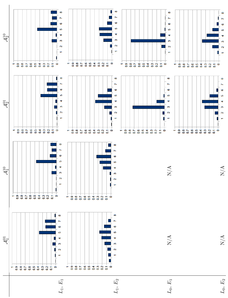
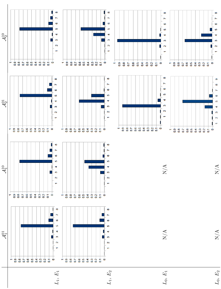
Appendix
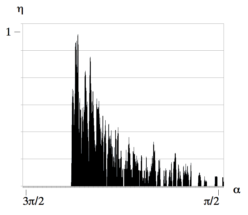
Distributions of cell in-degrees for automata and after - and -excitations are shown in Figs. 18 and 19. Calculations are done separately for cells lyings inside stimulation disc (Fig. 18) and outside the disc (Fig. 19). Each chart represents distribution of cell in-degrees, where horizontal axis is a number of incoming links and vertical axis is a ratio of cells with given in-degree to a total number of cells in the analysed domain.