Abstract

A numerical investigation of a non-commutative field theory defined via the spectral action principle is conducted. The construction of this triple relies on an 8-dimensional Clifford algebra. Following to the standard procedure of non-commutative geometry, the spectral action is computed for the product of the triple $(\mathcal{A}_{4},\mathcal{H}_{4},\mathcal{D}_{4})$ with a matrix-valued spectral triple. Using Monte Carlo simulation we study various quantities such as the energy density, the specific heat density and some order parameters varying the matrix size and the independent parameters of the model.

1 Introduction

The main object of this work is a particular non-commutative field theory which is derived using the spectral action principle and then treated numerically. Non-commutativity can be found in many fields of physics like quantum field theories, string theory, condensed matter physics. The first application of non-commutativity into physics is dated from the middle of the last century inspired by the ideas of quantum mechanics, where starting from classical mechanics, the commutative algebra of functions on the phase space is replaced by a non-commutative operator algebra on a Hilbert space. The duality between ordinary spaces $M$ and proper commutative algebras is expressed by the Gel’fand-Naimark theorem which states the fact that the algebra of all continuous functions on $M$ is the only possible type of commutative $C^{*}$-algebra. Additionally, given a commutative $C^{*}$-algebra $C$, it is possible to reconstruct a Hausdorff topological space $M$ in order to obtain that $C$ is the algebra of continuous functions on $M$. The study of commutative $C^{*}$-algebras is equivalent to the study of topological Hausdorff spaces. The previous duality has inspired the identification, in non-commutative geometry, of some algebraical objects as a category of non-commutative topological spaces. Alain Connes [1], one of the founders of non-commutative geometry, has proposed a candidate for the objects of such category, the spectral triples $(\mathcal{A},\mathcal{H},\mathcal{D})$ [2], composed by an algebra $\mathcal{A}$, an Hilbert space $\mathcal{H}$ on which $\mathcal{A}$ is represented and an selfadjoint operator $\mathcal{D}$. In fact, every compact oriented Riemannian manifold can be used to define a spectral triple, this kind of manifold $M$ characterizes a Dirac operator on self-adjoint Clifford module bundles over $M$. Connes, after a conjecture in 1996 [6] and some considerable attempts of Rennie and Varilly [7], proved the so called reconstruction theorem [3] for commutative spectral triples satisfying various axioms, showing that exists a compact oriented smooth manifold $X$ such that $A=C^{\infty}(X)$ is the algebra of smooth functions on $X$ and every compact oriented smooth manifold emerges in this way. Pushed by the aim of reformulating the standard model of particles in a non-commutative way [4, 6], Connes has introduced the almost-commutative spectral triple extending the axioms of the reconstruction theorem to a non-commutative algebra. A first attempt to formulate a field theory for a truly non-commutative algebra was obtained replacing in the usual field theory action the point-wise multiplication of the fields with a non-commutative one, namely a $\star$-product. The fields now belongs to $\mathbb{R}^{4}_{\Theta}$, a vector space defined by an enough regular class functions on $\mathbb{R}^{4}_{\Theta}$ equipped with the Moyal product:

$$(f\star g)(x)=\int\int d^{4}y\frac{d^{4}k}{(2\pi)^{4}}f(x+\frac{1}{2}\Theta\cdot k)g(x+y)e^{i\langle k,y\rangle}$$

Where $\Theta$ is a skew-symmetric matrix. A very important question about non-commutative quantum field theory [8], is whether or not the quantum theory is well-defined or in other words if it is renormalizable or not. At first sight, the non-locality of the non-commutate action induced by the $\star$-product in the position space can induce us to fear some problems for the renormalization. In fact it was discovered [8] that after computing the Feynman rules for such theory and deriving the loop amplitude we find that the non-local interaction terms in the action induce an oscillatory factors (involving loop momenta) in the Feynman integrals. Studying the structure of Feynman diagrams for the action, Filk [13] has showed that are present two types of loop diagram the planar and non-planar diagrams. The planar diagrams do not have this oscillatory factors coming from the non-local interaction terms, and therefore the corresponding integrals are the same as in usual quantum field theory. On the other hand, all non-planar diagrams have the oscillatory factors involving loop momenta. Due to this terms the renormalization of quantum field theories on the non-commutative $\mathbb{R}^{n}$ is not achieved and these models show a phenomenon called UV/IR-mixing [11]. Chepelev and Roiban [12] analyses UV/IR-mixing to all orders, the conclusion of the power-counting theorem is that field theories on non-commutative $\mathbb{R}^{n}$ are not renormalizable if the divergence of their commutative counterparts are higher than logarithmic.

A great step towards the non-commutative field theory was made when H.Grosse and R.Wulkenhaar [24], found a non-commutative $\varphi^{4}$-theory renormalizable action which develops additional marginal coupling, corresponding to an harmonic oscillator potential for the real-valued free field $\varphi$ on $\mathbb{R}^{4}_{\Theta}$ :

$$S[\varphi]=\int d^{4}x\left(\frac{1}{2}\varphi\star(-\Delta+\Omega^{2}\tilde{x}^{2}+\mu^{2})\star\varphi+\frac{\lambda}{4}\varphi\star\varphi\star\varphi\star\varphi\right)(x)$$

Where $x=2\Theta^{-1}\cdot x,\ \lambda\in\mathbb{R}\ \Omega\in[0,1]$, and $\mu$ is a real parameter. Using the Moyal matrix base, which turns the $\star$-product into a standard (infinite) matrix product, H.Grosse and R.Wulkenhaar were able to prove the perturbative renormalizability of the theory [25]. Afterward, R.Wulkenhaar et al. [14] found an alternative simpler normalization proof using multi-scale analysis in matrix base, showing the equivalence of various renormalization schemes. A last, but useful, renormalization proof was formulated using Symanzik type hyperbolic polynomials [16].

The non-commutative model treated in this work is a sort of extension, via spectral action principle, of the scalar W-G model, in which we are interested to formulate a Yang-Mills theory in renormalizable way on Moyal space. We can expect that usual Yang-Mills theory on Moyal space without modifications of the action by something similar to an oscillator potential, to be not renormalizable [11]. Additionally, the Moyal space with usual Dirac operator is a spectral triple, the corresponding spectral action was computed in [17], with the result that it is the usual not renormalizable action on Moyal plane. In [18] H.Grosse and R.Wulkenhaar, in order to obtain a gauge theory with an oscillator potential via the spectral action principle, used a Dirac operator constructed using the statement $\mathcal{D}^{2}=H$ where the four dimensional Laplacian is substituted by the four dimensional oscillator Hamiltonian $H=-\Delta+\Omega^{2}||x||^{2}$. The idea behind is that the spectral dimension is defined through the Dirac operator so the spectral dimension defined by such Dirac operator is related to the harmonic oscillator phase space dimension. It turns out that to write down an Dirac operator, so that its square equals the 4D harmonic oscillator Hamiltonian, is an easy task using eight dimension Clifford algebra. In addition, can be shown that using this Dirac operator on 4D-Moyal space, is possible define an eight-dimensional spectral triple. After defined the Dirac operator with the desired spectrum it is considered the total spectral triple as the tensor product of the ”oscillating” spectral triple $(\mathcal{A}_{4},\mathcal{H}_{4},\mathcal{D}_{4})$ with an almost-commutative triple and then is perform the previous described procedure of non-commutative geometry to compute the spectral action. We notice that matrix algebra introduces an extension of the standard potential in the commutative case, in fact the scalar field $\phi$ and the $X_{\mu}$ fields are present together in a potential of the form $(\alpha X_{\mu}\star X^{\mu}+\beta\bar{\varphi}\star\varphi-1)^{2}$, with $\alpha,\beta\in\mathbb{R}^{+}$ and $X_{\mu}(x)=(\Theta^{-1})_{\mu}^{\nu}x_{\nu}+A_{\mu}(x)$ is a covariant coordinate.

The high non-triviality of the vacuum makes very difficult to explicit the vacuum configuration of the system in [20] A. de Goursac, J.C. Wallet, and R. Wulkenhaar, using the matrix base formalism, have found an expressions from vacuum solutions deriving them from the relevant solutions of the equations of motion. Although, the complexity of the vacuum configuration makes the perturbative approach very complicated, in order to conduct some investigations will be considered a non-perturbative scheme using a discretized matrix model of the action in which the fields become matrices, the star product become the matrix multiplication and the integral turns in a matrix trace.

Now comes in to play the numerical treatment, the standard method is to approximate the space by discrete points, for example using a lattice approximation and then calculate the observables over that set of points [21]. Since an approximation in the position space is not suitable due to the oscillator factor of the Moyal product, instead the lattice approximation, will be used the matrix Moyal base, which was already used in the first renormalization proof of $\varphi^{4}$-model restricted to finite matrices. Hence, will be performed a Monte Carlo simulation studying some statistical quantity such the energy density and specific heat varying the parameters $\Omega,\frac{\chi_{-1}}{\chi_{0}},\alpha$ and gathering some informations on the various contributions of the fields to the action. The simulations are quite cumbersome due the complexity of the action and the number of independent matrices to handle but we are able to get an acceptable balance between the computation precision and the computation time. For the simulations is applied a standard Metropolis-Monte Carlo algorithm [22] with various estimators for the error and for the autocorrelation time of the samples. In general we chose the range of parameters in order to avoid problems with the thermalization process, obtaining numerical simulations where is enough to wait a relative small number of Monte Carlo steps to compute independent results from the initial conditions. we are interested on the continuous limit that correspond to matrices of infinite size. We will consider various size of the matrices expecting a stabilization of the values of observables like the energy density, increasing the matrix size. In order to find same possible phase transitions will be used the specific heat which is a measure of the dispersion of the energy. The phase transitions are registered as peaks of the specific heat, increasing the matrices size.

2 8-dim spectral action

In this section will be computed a spectral action starting from a non-commutative spectral triple. The feature of this particular triple is the choice of a 4-dimension Harmonic Dirac operator. The idea behind this construction [18] is to relate the Dirac operator with the oscillator Hamiltonian operator. Roughly speaking, we look at the Dirac operator as a generalization of the Laplace operator so we have $\mathcal{D}^{2}\approx H$. Considering the spectrum $\omega(2n+1)$ $n\in N$ of the one-dimensional harmonic oscillator Hamiltonian $H$, can be deduced that $H^{-1}$ is a non-commutative infinitesimal of order one. The non-commutative dimension of a spectral triple, equipped with the 4D Harmonic Dirac operator $\mathcal{D}^{2}_{4}=H_{4}$, is fixed by the non-commutative order of the inverse operator $\mathcal{D}^{-1}$ which is eight not four. This occurrence connects the spectral dimension to the phase space dimension instead the one of the configuration space [5]. In order to construct such Harmonic Dirac operator and the spectral triple we will work in the framework of the generalized $n$-dimensional harmonic operators. Will be studied the 4-dimensional case in order to construct the non-commutative spectral triple which is starting point for the field theory we are interested in. Having the 4-dimensional Harmonic Dirac operator with harmonic oscillator spectrum, to implement the Higgs mechanism we will consider the tensor product of the non-commutative triple with a finite Connes-Lott type spectral triple [10]. We will fluctuate the total Dirac operator following the standard machinery [23, 6] of non-commutative geometry to get ”Gauged” Dirac operator. Thus we will proceed to compute the spectral action in which are present two U(1)-Moyal Yang-Mills fields unified with a complex Higgs field.

3 Harmonic Dirac operators

1

The Harmonic Dirac operator in $n$-dimensions can be defined using the Clifford algebra of $\mathbb{R}^{2n}$ represented on the Hilbert space $\mathbb{C}^{2^{n}}$, it is very useful to consider $n$-dimensional fermionic annihilation and creation operators $b_{\mu}$, $b_{\nu}^{\dagger}$ and $n$-dimensional bosonic annihilation and creation operators $a_{\mu}$, $a^{\dagger}_{\nu}$ satisfying for $\mu,\nu=1,\cdots,n$:

$$[a_{\mu},a_{\nu}]=[a^{\dagger}_{\mu},a^{\dagger}_{\nu}]=0, [a_{\mu},a^{\dagger}_{\nu}]=\delta_{\mu\nu}$$ (1)

$$\{b_{\mu},b_{\nu}\}=\{b_{\mu}^{\dagger},b_{\nu}^{\dagger}\}=0, \{b_{\mu},b_{\nu}^{\dagger}\}=\delta_{\mu\nu}$$ (2)

Where $a_{\mu}=\frac{1}{\sqrt{2\omega}}(\omega x_{\mu}+\partial_{\mu}),\ a_{\mu}^{\dagger}=\frac{1}{\sqrt{2\omega}}(\omega x_{\mu}-\partial_{\mu})$. Using this operators is possible to construct a Dirac operator as:

$$\mathcal{D}_{n}=-i\sqrt{2\omega}\delta^{\mu\nu}a_{\mu}^{\dagger}\otimes b_{\nu}+i\sqrt{2\omega}\delta^{\mu\nu}a_{\mu}\otimes b_{\nu}^{\dagger}=i\frac{d}{dx_{\mu}}\otimes(b_{\mu}+b_{\mu}^{\dagger})+i\omega x^{\mu}\otimes(b_{\mu}-b^{\dagger}_{\mu})$$ (3)

summed over repeated index. We can define the fermionic part of the Hilbert space on which the Dirac operator (3) acts starting from the vacuum state by subsequent applications of the fermionic creation operators $b_{\nu}^{\dagger}$ on the vacuum $b|0\rangle=0$, using the anti-commutation relations (2) defining $\Lambda(\mathbb{C}^{n})$. The complete Hilbert space is $\mathcal{H}_{n}=S(\mathbb{R}^{n})\otimes\Lambda(\mathbb{C}^{n})$. Beside, we can define a grading operator $\chi_{n}$ as:

$$\chi_{n}=\textbf{I}\otimes\prod^{n}_{\mu=1}(b_{\mu}b^{\dagger}_{\mu}-b_{\mu}b^{\dagger}_{\mu})$$ (4)

Using the relations (1)-(2) we can compute the square the Dirac operator (3) as:

$$\mathcal{D}_{n}^{2}=2\omega a^{\dagger}_{\mu}a^{\mu}\otimes\textbf{I}-2\omega\textbf{I}\otimes b^{\dagger}_{\mu}b^{\mu}=2\omega N_{B}\otimes\textbf{I}-2\omega\textbf{I}\otimes N_{F}$$ (5)

Where $N_{F}$ and $N_{B}$ are the number operators. In this form it easy to see that $\mathcal{D}^{2}_{n}$, being a ”difference” between fermionic and bosonic number operator, has only one zero mode corresponding to the vacuum state. For practical reasons it is convenient write $\mathcal{D}^{2}_{n}$ as:

$$\mathcal{D}_{n}^{2}=\omega\delta^{\mu\nu}(a^{\dagger}_{\mu}a_{\nu}+a_{\nu}a^{\dagger}_{\mu})\otimes\textbf{I}-2\omega\textbf{I}\otimes\delta^{\mu\nu}(b^{\dagger}_{\mu}b_{\nu}-b_{\nu}b^{\dagger}_{\mu})=H_{n}\otimes\textbf{I}+\omega\otimes\Sigma_{n}$$ (6)

where in $H_{n}$ we can recognize the harmonic oscillator Hamiltonian and the spin operator $\Sigma_{n}$. The universality property of the Clifford algebra grants the existence of an isomorphism between the 2$n$-dimensional Clifford algebra and the Hilbert space $\mathcal{H}_{n}=S(\mathbb{R}^{n})\otimes\mathbb{C}^{2^{n}}$. In this representation the Dirac operator is:

$$\mathcal{D}_{n}=i\Gamma^{\mu}\partial_{\mu}+\omega\Gamma^{\mu+n}x_{\mu}$$ (7)

Where $\Gamma^{\mu}$ turns to be $\Gamma^{\mu}=(b_{\mu}+b^{\dagger}_{\mu})$, $\Gamma^{\mu+n}=i(b^{\dagger}_{\mu}-b_{\mu})$ which satisfy the relations:

$$\Gamma_{a}\Gamma_{b}+\Gamma_{b}\Gamma_{a}=2\delta_{ab}\ \textrm{with}\ a,b=1,\cdots,2n$$ (8)

Beside, the grading operator is represented as:

$$\chi_{n}=(-i)^{n}(-1)^{\frac{n(n-1)}{2}}\otimes\Gamma_{1}\cdots\Gamma_{2n}$$ (9)

4 An harmonic spectral triple for the Moyal plane

In the framework of non-commutative field theories on 4-dimensional Moyal plane has been proved [24, 25] that the introduction of an harmonic oscillator term makes a $\phi^{4}$-model on 4-dimensional Moyal plane renormalizable. Such oscillator term can be written as:

$$H_{m}=-\frac{\partial^{2}}{\partial x_{\mu}\partial x^{\mu}}+\Omega^{2}\tilde{x}_{\mu}\tilde{x}^{\mu}+m^{2}$$ (10)

where $\tilde{x}_{\mu}:=2(\Theta^{-1})_{\mu\nu}x^{\nu}$, $\Theta$ can be chosen as two copies of the Pauli matrix $\Theta=i\theta\sigma_{2}\otimes\textbf{I}_{2}$ or explicitly:

$$\Theta=\left(\begin{array}[]{cccc}0&\theta&0&0\\ -\theta&0&0&0\\ 0&0&0&\theta\\ 0&0&-\theta&0\end{array}\right),\ \theta\in\mathbb{R}$$ (11)

With this choice we have $\Theta^{-1}=-\frac{i\sigma_{2}}{\theta}\otimes\textbf{I}_{2}$. Quantum mechanics tell us that in the Hilbert space $L^{2}(\mathbb{R}^{4})$ exists an orthonormal basis $\psi_{s},\ s\in\mathbb{R}^{4}$ of eigenfunctions of $H_{m}$ with eigenvalues

$$\lambda_{s}(m)=\left(\frac{4\Omega}{\theta}\left(s+2+\frac{\theta m^{2}}{2\Omega}\right)\right),\ s\in\mathbb{N}$$ (12)

The inverse $H^{-1}_{m}$ extends to a selfadjoint compact operator on $L^{2}(\mathbb{R}^{4})$ with eigenvalues $\lambda^{-1}_{s}(m)$. If we look at the trace the operator $H^{-4}_{m}$ we find:

$$\operatorname{Tr}(H^{-s}_{m})=\sum_{n=0}^{\infty}(n+3)(n+2)(n+1)(\lambda_{n}(m))^{s}$$ (13)

Which is derived simply from the number of possibilities to express $s$ as a sum of four ordered natural numbers. This means that $H^{-4}$ belongs to the Dixmier trace ideal $L^{(1,\infty)}(L^{2}(\mathbb{R}^{4}))$ of compact operators and the relation $\mathcal{D}^{2}=H$ implies that the 4-dimensional Moyal space has spectral dimension 8. From the previous section, we can define a proper Dirac operator just considering the 4-dimensional case obtaining a Dirac operator built from a 8-dimensional Cifford algebra:

$$\mathcal{D}_{4}=i\Gamma_{\mu}\partial_{\mu}+\Omega\Gamma_{\mu+4}\tilde{x}_{\mu}$$ (14)

Here, the $\Gamma_{k}\in M_{16}(\mathbb{C}),k=1,...,8$ are the generators of the 8-dimensional real Clifford algebra, satisfying

$$\Gamma_{k}\Gamma_{l}+\Gamma_{l}\Gamma_{k}=2\delta_{kl}\textbf{I}$$ (15)

We take the Hilbert space $\mathcal{H}_{4}=S^{2}(\mathbb{R}^{4},\mathcal{S})=L^{2}(\mathbb{R}^{4})\otimes\mathbb{C}^{16}$ of Schwartz functions of spinors over 4-dimensional euclidean space. Accordingly with (8) for $\psi\in\mathcal{H}_{4}$ we obtain:

$$\mathcal{D}^{2}_{4}\psi=\left((-\Delta+\Omega^{2}\tilde{x}_{\mu}\tilde{x}^{\mu})\textbf{I}+\Sigma\right)\psi\ ,\ \Sigma:=-i\Omega(\Theta^{-1})^{\mu\nu}[\Gamma_{\mu},\Gamma_{\nu+4}]$$ (16)

with $\Delta=\partial^{\mu}\partial_{\mu}$. As algebra we chose the Moyal algebra $\mathbb{R}^{4}_{\Theta}$:

$$\mathcal{A}_{4}=\mathbb{R}_{\Theta}^{4}=(\mathcal{S}(\mathbb{R}^{4}),\star)$$ (17)

where $(\mathcal{S}(\mathbb{R}^{4}),\star)$ is the algebra of the Schwartz functions on $\mathbb{R}^{4}$, with the Moyal product

$$(f\star g)(x)=\int\int d^{4}y\frac{d^{4}k}{(2\pi)^{4}}f(x+\frac{1}{2}\Theta\cdot k)g(x+y)e^{i\langle k,y\rangle}\ ,\ f,g\in\mathcal{A}_{4}$$ (18)

The representation of the algebra $\mathcal{A}_{4}$ on $\mathcal{H}_{4}$ is by component-wise diagonal Moyal product [26] $\star:\mathcal{A}_{4}\times\mathcal{H}_{4}\to\mathcal{H}_{4}$. The Moyal product can be extended to constant functions using another representation of the product with the integral representation of the Dirac distribution. Taking in account, for smooth spinors, the identity $2x^{\mu}\psi=x\star\psi+\psi\star x$ and the relation

$$[x^{\nu},f]_{\star}=i\Theta^{\nu\rho}\partial_{\rho}$$ (19)

we compute the commutator of that action with the Dirac operator

$$\begin{array}[]{l}\mathcal{D}_{4}(f\star\psi)-f\star(\mathcal{D}_{4}\psi)\\ =i\Gamma^{\mu}((\partial_{\mu}f)\star\psi+f\star\partial_{\mu}\psi)+\frac{1}{2}\Omega\Gamma^{\mu+4}(\tilde{x}_{\mu}\star(f\star\psi)+(f\star\psi)\star\tilde{x}_{\mu})\\ -i\Gamma^{\mu}f\star\partial_{\mu}\psi-\frac{1}{2}\Omega\Gamma^{\mu+4}(f\star(\tilde{x}_{\mu}\star\psi)+f\star(\psi\star\tilde{x}_{\mu}))\\ =i(\Gamma^{\mu}+\Omega\Gamma^{\mu+4})(\partial_{\mu}f)\star\psi.\end{array}$$ (20)

The previous commutator confirms that $(\mathcal{A}_{4},\mathcal{H}_{4},\mathcal{D}_{4})$ satisfy the main axioms of spectral triple, in fact the commutator is bounded and due to its commutation with Moyal multiplication, order-one condition is fulfilled. Now we introduce a very useful relation connected to the heat kernel type expansion associated to a regular spectral triple taken from [19]. This relation will be used later in order to compute the spectral action. Considering a regular non-unital spectral triple $(\mathcal{A},\mathcal{H},\mathcal{D},J)$ and two pseudo-differential operator $A_{0}\in\Psi_{0}(\mathcal{A})$ $A_{1}\in\Psi_{1}(\mathcal{A})$ of order respectively 0 and 1. We consider the following decomposition:

$$e^{-t(\mathcal{D}^{2}+A_{0}+A_{1})}=\sum_{j=0}^{4}(-1)^{j}E_{j}(t)-t^{5}R$$ (21)

Using Duhamel principle [27]

$$e^{-t(A+B)}=e^{-tA}-t\int_{0}^{1}ds\ e^{-st(A+B)}Be^{-(1-s)tA}$$ (22)

we can identify:

$$E_{0}(t) = e^{-t\mathcal{D}^{2}}$$

$$\ E_{j}(t) = \int_{\Delta_{j}}d^{j}s\ e^{-s_{1}t\mathcal{D}^{2}}(A_{0}+A_{1})e^{-(s_{2}-s_{1})t\mathcal{D}^{2}}\cdots(A_{0}+A_{1})e^{-(1-s_{j})t\mathcal{D}^{2}}$$

(23)

and

$$R=\int_{\Delta_{5}}ds_{1}ds_{2}ds_{3}ds_{4}ds_{5}e^{-s_{1}t(\mathcal{D}^{2}+A_{0}+A_{1})}(A_{0}+A_{1})e^{-(s_{2}-s_{1})t\mathcal{D}^{2}}(A_{0}+A_{1})$$

$$\times e^{-(s_{3}-s_{2})t\mathcal{D}^{2}}(A_{0}+A_{1})e^{-(s_{4}-s_{3})t\mathcal{D}^{2}}(A_{0}+A_{1})e^{-(s_{5}-s_{4})t\mathcal{D}^{2}}(A_{0}+A_{1})e^{-(1-s_{5})t\mathcal{D}^{2}}$$

The domains of the integrals $\Delta_{j}$ are the $j$-simplex:

$$\Delta_{j}=\{s\in\mathbb{R}^{j};0\leq s_{1}\leq s_{2}\leq s_{1}\leq\cdots\leq s_{j}\leq 1\}\simeq\{s\in\mathbb{R}^{j+1};s_{i}\geq 0,\sum_{i=0}^{j}s_{i}=1\}$$ (25)

Taking in account the relation:

$$\left[e^{-t\mathcal{D}^{2}},A\right]=\int_{0}^{1}ds\frac{d}{ds}\left(e^{-ts\mathcal{D}^{2}}Ae^{-t(1-s)\mathcal{D}^{2}}\right)=-t\int_{0}^{1}dse^{-ts\mathcal{D}^{2}}\left[\mathcal{D}^{2},A\right]e^{-t(1-s)\mathcal{D}^{2}}$$ (26)

and considering the trace in [19] is computed the leading term of $e^{-t(\mathcal{D}^{2}+A_{0}+A_{1})}$ for $t\to 0$:

$$\operatorname{Tr}(e^{-t(\mathcal{D}^{2}+A_{0}+A_{1})})$$

$$=\textrm{Tr}\Big{(}\Big{\{}1-t(A_{0}+A_{1})+\frac{t^{2}}{2}(A^{2}_{0}+A_{1}A_{0}+A_{0}A_{1}+A^{2}_{1})$$

$$-\frac{t^{3}}{6}(A_{0}\left[\mathcal{D}^{2},A_{1}\right]+A_{1}\left[\mathcal{D}^{2},A_{0}\right]+A_{1}\left[\mathcal{D}^{2},A_{1}\right]+A_{0}A^{2}_{1}+A_{1}A_{0}A_{1}+A_{1}^{2}A_{0}$$

$$+A^{3}_{1})+\frac{t^{4}}{24}(A_{1}\left[\mathcal{D}^{2}\left[\mathcal{D}^{2},A_{0}\right]\right]+2A^{2}_{1}\left[\mathcal{D}^{2},A_{1}\right]+A_{1}\left[\mathcal{D}^{2},A_{1}\right]A_{1}+A_{1}^{4}\Big{)}e^{-t\mathcal{D}^{2}}\Big{\}}$$

$$+\mathcal{O}(\sqrt{t})$$ (27)

5 4-dimensional harmonic Yang-Mills model

Following the Connes-Lott models, in order to implement the Higgs mechanism, we consider the total spectral triple as the tensor product of the 8-dimensional spectral triple $(\mathcal{A}_{4},\mathcal{H}_{4},\mathcal{D}_{4},\Gamma_{9})$ with the two point Connes-Lott like spectral triple $(\mathbb{C}\otimes\mathbb{C},\mathbb{C}^{2},M\sigma_{1})$. The total Dirac operator of the product triple is:

$$\mathcal{D}_{T}=\mathcal{D}_{4}\otimes\textbf{I}+\Gamma_{9}\otimes M\sigma_{1}$$ (28)

Or explicitly:

$$\mathcal{D}_{T}=\left(\begin{array}[]{cc}\mathcal{D}_{4}&M\Gamma_{9}\\ M\Gamma_{9}&\mathcal{D}_{4}\end{array}\right)$$ (29)

The algebra becomes $\mathcal{A}_{T}=\mathcal{A}_{4}\oplus\mathcal{A}_{4}$ and acts by diagonal star multiplication (18) on $\mathcal{H}_{T}=\mathcal{H}_{4}\oplus\mathcal{H}_{4}$. The fluctuated Dirac operator is found using $\mathcal{D}_{A}=\mathcal{D}_{T}+\Sigma_{i}a_{i}[\mathcal{D}_{T},b_{i}]$ with $a_{i},b_{i}\in\mathcal{A}_{T}$ of the form $(f,g)$, the computation of the commutator $\mathcal{D}_{T}$ with $(f,g)$ gives:

$$[\mathcal{D}_{T},(f,g)]=\left(\begin{array}[]{cc}i(\Gamma^{\mu}+\Omega\Gamma^{\mu+4})L_{\star}(\partial_{\mu}f)&M\Gamma_{9}L_{\star}(f-g)\\ M\Gamma_{9}L_{\star}(g-f)&i(\Gamma^{\mu}+\Omega\Gamma^{\mu+4})L_{\star}(\partial_{\mu}g)\end{array}\right)$$ (30)

$L_{\star}(f)\psi=f\star\psi$ is the left Moyal multiplication. From the commutator we deduce that the form of selfadjoint fluctuated Dirac has to be:

$$\mathcal{D}_{A}=\left(\begin{array}[]{cc}\mathcal{D}_{4}+(\Gamma_{\mu}+\Omega\Gamma_{\mu+4})L_{\star}(A^{\mu})&\Gamma_{9}L_{\star}(\phi)\\ \Gamma_{9}L_{\star}(\bar{\phi})&\mathcal{D}_{4}+(\Gamma_{\mu}+\Omega\Gamma_{\mu+4})L_{\star}(B^{\mu})\end{array}\right)$$ (31)

Where $\phi\in\mathcal{A}_{4}$ is the Higgs complex field and $A_{\mu},B_{\mu}\in\mathcal{A}_{4}$ are real fields. The spectral action computation needs the square of $\mathcal{D}_{A}$:

$$\mathcal{D}^{2}_{A}=\left(\begin{array}[]{cc}(H^{2}_{0}+L_{\star}(\phi\star\varphi))1+\Sigma+F_{A}&i(\Gamma_{\mu}+\Omega\Gamma_{\mu+4})\Gamma_{9}L_{\star}(D^{\mu}\phi)\\ i(\Gamma_{\mu}+\Omega\Gamma_{\mu+4})\Gamma_{9}L_{\star}(\overline{D^{\mu}\phi})&(H^{2}+L_{\star}(\phi\star\phi))1+\Sigma+F_{B}\end{array}\right)$$ (32)

with

$$D_{\mu}\phi = \partial_{\mu}\phi-iA_{\mu}\star\phi+i\phi\star B_{\mu}$$ (33)

$$F_{A} = \{\mathcal{D}_{4},(\Gamma_{\mu}+\Omega\Gamma_{\mu+4})L_{\star}(A^{\mu})\}+(\Gamma_{\mu}+\Omega\Gamma_{\mu+4})(\Gamma_{\nu}+\Omega\Gamma_{\nu+4})L_{\star}(A^{\mu}\star A^{\nu})$$ (34)

$$= \{L_{\star}(A^{\mu}),i\partial_{\mu}+\Omega^{2}M_{\bullet}(x_{\mu})\}+(1+\Omega^{2})L_{\star}(A_{\mu}\star A^{\mu})$$

$$+ i\left(\frac{1}{4}[\Gamma_{\mu},\Gamma_{\nu}]+\frac{1}{4}\Omega^{2}[\Gamma_{\mu+4},\Gamma_{\nu+4}]+\Omega\Gamma_{\mu}\Gamma_{\nu+4}\right)L_{\star}(F^{\mu\nu}_{A}),$$

$(M_{\bullet}(\tilde{x}_{\mu})\psi)(x)=\tilde{x}_{\mu}\psi(x)$ is ordinary pointwise multiplication and $F_{B}$ is obtained just replacing $A$ with $B$. We can recognize in previous expression the field strength $F^{A}_{\mu\nu}=\partial_{\mu}A_{\nu}-\partial_{\nu}A_{\mu}-i(A_{\mu}\star A_{\nu}-A_{\nu}\star A_{\mu})$

5.1 Spectral action

Recalling the spectral action principle, the bosonic action can be defined exclusively by the spectrum of the Dirac operator. The general form for such bosonic action is:

$$S(\mathcal{D}_{A})=\textrm{Tr}\chi(\mathcal{D}^{2}_{A})$$ (35)

Where $\chi$ is a regularization function $\chi:R_{+}\to R_{+}$ for which trace exists.
The trace in (35) is defined on $\mathcal{B}(L^{2}(\mathbb{R}^{4}))$ by

$$\operatorname{Tr}(A)=\int_{\mathbb{R}^{4}}dx\ A(x,x)$$ (36)

together with the matrix trace including the Clifford algebra. By Laplace transformation one has

$$S(\mathcal{D}_{A})=\int_{0}^{\infty}dt\operatorname{Tr}(e^{-t\mathcal{D}^{2}_{A}})\tilde{\chi}(t)$$ (37)

where $\tilde{\chi}$ is the inverse Laplace transform of $\chi(s)$,

$$\chi(s)=\int_{0}^{\infty}dte^{-st}\tilde{\chi}(t).$$ (38)

The trace in (37) is given by:

$$\operatorname{Tr}(e^{-t\mathcal{D}^{2}_{A}})=\int_{\mathbb{R}^{4}}dx\ \textrm{tr}(e^{-t\mathcal{D}^{2}_{A}})(x,x)$$ (39)

Assuming the trace of the heat kernel $e^{-t\mathcal{D}^{2}_{A}}$ has an asymptotic expansion

$$\operatorname{Tr}(e^{-t\mathcal{D}^{2}_{A}})=\sum^{\infty}_{n=-\delta}a_{n}(\mathcal{D}^{2}_{A})t^{n}\ ,\ \delta\in\mathbb{N}$$ (40)

we obtain replacing the previous expansion into (37)

$$S(\mathcal{D}_{A})=\sum_{n=-\delta}^{\infty}a_{n}(\mathcal{D}^{2}_{A})\int_{0}^{\infty}dt\ t^{n}\tilde{\chi}(t)$$ (41)

To compute the integrals we have to consider separately the cases $n\notin\mathbb{N}$ and $n\in\mathbb{N}$:

$$\chi_{n}=\Bigg{\{}\begin{array}[]{ll}\frac{1}{\Gamma(-n)}\int_{0}^{\infty}ds\ s^{-n-1}\chi(s)&\textrm{for}\ n\notin\mathbb{N}\\ (-1)^{n-\delta}\chi^{(n)}(0)&\textrm{for}\ n\in\mathbb{N}\end{array}$$ (42)

Due to the nature of the $\chi(t)$ function (usually one chose a characteristic function), we can assume $\chi(0)$ much bigger then the derivatives $\chi^{(m)}(0)$ for any $m>0$ appearing in (42). Consequently in the expansion (40) we will take in account only the finite or singular part for $t\to 0$

Our strategy to compute the action is to use the relation (27), therefore after explicitly expressed $A_{0}$ and $A_{1}$ we proceed to the calculus of the traces and in the end we will identify the leading part of the action comparing the result with the expansions (40)-(41). We can identify the operators $A_{0}$ and $A_{1}$ appearing in the (27) as follow:

$$A_{0}=\left(\begin{array}[]{cc}L_{\star}(V_{A,\phi})\textbf{I}+L_{\star}(F_{A}^{\mu\nu})\Gamma^{\Omega}_{\mu\nu}&i(\Gamma^{\mu}+\Omega\Gamma^{\mu+4})\Gamma_{9}L_{\star}(D_{\mu}\phi)\\ i(\Gamma^{\mu}+\Omega\Gamma^{\mu+4})\Gamma_{9}L_{\star}(\overline{D_{\mu}\phi})&L_{\star}(V_{B,\phi})\textbf{I}+L_{\star}(F_{B}^{\mu\nu})\Gamma^{\Omega}_{\mu\nu}\end{array}\right)$$ (43)

$$A_{1}=\left(\begin{array}[]{cc}2i(1+\Omega^{2})L_{\star}(A^{\mu})\nabla_{\mu}^{(\Omega)}&0\\ 0&2i(1+\Omega^{2})L_{\star}(B^{\mu})\nabla_{\mu}^{(\Omega)}\end{array}\right)$$ (44)

with

$$V_{A,\phi}=\phi\star\bar{\phi}+(1+\Omega^{2})(i\partial_{\mu}A^{\mu}+A_{\mu}\star A^{\mu}),\ V_{B,\phi}=\bar{\phi}\star\phi+(1+\Omega^{2})(i\partial_{\mu}B^{\mu}+B_{\mu}\star A^{\mu})$$ (45)

$\nabla_{\mu}^{(\Omega)}$ are define as $\nabla_{\mu}^{(\Omega)}=\frac{1}{1+\Omega^{2}}\left(\partial_{\mu}-i\Omega^{2}M_{\bullet}(\tilde{x}_{\mu})\right)$. We are allowed to split the traces in two parts a matrix trace and the continuous one. After the matrices trace computations we obtain [19] for the $A$ field:

$$\textrm{Tr}(e^{-t\mathcal{D}_{A}^{2}})$$

$$=\Bigg{\{}16\cosh^{4}(t\Omega)\textrm{tr}(e^{-tH_{4}^{2}})-tT(16V_{A,\phi})-t\mathcal{T}_{\mu}(32i(1+\Omega^{2})A^{\mu})$$

$$+\frac{t^{2}}{2}\mathcal{T}\Big{(}16V_{A,\phi}\star V_{A,\phi}+16(1+\Omega^{2})D_{\mu}\phi\star\overline{D^{\mu}\phi}+8(1+\Omega^{2})F_{\mu\nu}^{A}F^{\mu\nu}_{A}$$

$$+32i(1+\Omega^{2})A^{\mu}\star\partial_{\mu}V_{A,\phi}\Big{)}$$

$$+\frac{t^{2}}{2}\mathcal{T}_{\mu}\Big{(}32i(1+\Omega^{2})A^{\mu}\star V_{A,\phi}+32i(1+\Omega^{2})V_{A,\phi}\star A^{\mu}$$

$$-64(1+\Omega^{2})^{2}A^{\nu}\star\partial_{\nu}A^{\mu}\Big{)}+\frac{t^{2}}{2}\mathcal{T}_{\mu\nu}\left(-64(1+\Omega^{2})^{2}A^{\mu}\star A^{\nu}\right)$$

$$-\frac{t^{3}}{6}\mathcal{T}_{\mu\nu}\Big{(}-64(1+\Omega^{2})^{2}V_{A,\phi}\star\partial^{\mu}A^{\nu}-64i(1+\Omega^{2})^{2}A^{\nu}\star\partial^{\nu}V_{A,\phi}$$

$$+64(1+\Omega^{2})^{3}A_{\rho}\star(\delta^{\rho\mu}\triangle A^{\nu}+2\partial^{\rho}\partial^{\mu}A^{\nu})$$

$$-64(1+\Omega^{2})^{2}(V_{A,\phi}\star A^{\mu}\star A^{\nu}+A^{\mu}\star V_{A,\phi}\star A^{\nu}+A^{\mu}\star A^{\nu}\star V_{A,\phi})$$

$$-128i(1+\Omega^{2})^{3}\left(A^{\rho}\star(\partial_{\rho}A^{\mu})\star A^{\nu}+A^{\rho}\star A^{\mu}(\partial_{\rho}A^{\nu}\right)\Big{)}$$

$$-\frac{t^{3}}{6}\mathcal{T}_{\mu\nu\rho}\left(128(1+\Omega^{2})^{3}A^{\mu}\star\partial^{\nu}A^{\rho}-128i(1+\Omega^{2})^{3}A^{\nu}\star A^{\mu}\star A^{\rho}\right)$$

$$+\frac{t^{3}}{6}\tilde{\mathcal{T}}_{\mu\nu}\left(512i\Omega^{2}(1+\Omega^{2})(\Theta^{-1})^{\rho\nu}A^{\mu}\star A_{\rho}\right)$$

$$+\frac{t^{4}}{24}\mathcal{T}_{\mu\nu\rho\sigma}\Big{(}-256(1+\Omega^{2})^{4}A^{\mu}\star\partial^{\nu}\partial^{\rho}A^{\sigma}+512i(1+\Omega^{2})^{3}A^{\mu}\star A^{\nu}\star\partial^{\rho}A^{\sigma}$$

$$+256i(1+\Omega^{2})^{4}A^{\mu}\star(\partial^{\nu}A^{\rho})\star A^{\sigma}+256(1+\Omega^{2})^{4}A^{\mu}\star A^{\nu}\star A^{\rho}\star A^{\sigma}\Big{)}\Bigg{\}}$$

$$+\mbox{$B$ field contribution}\ +\mathcal{O}(\sqrt{t})$$ (46)

Where in order to simplify the notation we introduce the functions:

$$\mathcal{T}(f) = \textrm{Tr}_{L^{2}(\mathbb{R}^{4})}\left(L_{\star}(f)e^{-tH_{4}}\right)$$

$$\mathcal{T}_{\mu_{1}\cdots\mu_{k}}(f) = \textrm{Tr}_{L^{2}(\mathbb{R}^{4})}\left(L_{\star}(f)\nabla^{(\Omega)}_{\mu_{1}}\cdots\nabla^{(\Omega)}_{\mu_{k}}e^{-tH_{4}}\right)$$

$$\tilde{\mathcal{T}}_{\mu\nu}(f) = \textrm{Tr}_{L^{2}(\mathbb{R}^{4})}\left(L_{\star}(f)\nabla^{(\Omega)}_{\mu_{1}}\nabla^{(1)}_{\mu_{k}}e^{-tH_{4}}\right)$$ (47)

The contributions for the $B$ fields are obtained operating the following substitutions:

$$\left\{A_{\mu}\to B_{\mu},\ F^{A}_{\mu\nu}\to F^{B}_{\mu\nu},\ V_{A,\phi}\to V_{B,\phi},\ D_{\mu}\phi\leftrightarrow\overline{D^{\mu}\phi}\right\}$$ (48)

After the computation of the $\mathcal{T},\mathcal{T}_{\mu_{1}\cdots\mu_{k}}$ , we have all the ingredients required to compute the leading part of the action (35) replacing all the traces into the (27). Using the trace property of the star product and the identities

$$\tilde{z}_{\mu}\star f=\frac{1}{2}\{\tilde{z}_{\mu},f\}+\frac{1}{2}[\tilde{z}_{\mu},f]=\frac{1}{2}\{\tilde{z}_{\mu},f\}+i\partial_{\mu}f$$ (49)

$$\{\tilde{z}_{\mu},f\star g\}_{\star}=\{\tilde{z}_{\mu},f\}\star g-if\star\partial_{\mu}g$$ (50)

we get after some manipulations:

$$\textrm{Tr}(e^{-t\mathcal{D}^{2}})=2\cosh^{4}(\tilde{\Omega}t)$$

$$+\frac{1}{\pi^{2}(1+\Omega^{2})^{2}}\int d^{4}z\Bigg{\{}-\frac{1}{t}\Bigg{(}\left(\phi\star\bar{\phi}+\frac{4\Omega^{2}}{1+\Omega^{2}}(\tilde{X}^{A}_{\mu}\star\tilde{X}_{A}^{\mu}-\tilde{X}^{0}_{\mu}\star\tilde{X}_{0}^{\mu})\right)$$

$$+\left(\bar{\phi}\star\phi+\frac{4\Omega^{2}}{1+\Omega^{2}}(\tilde{X}^{B}_{\mu}\star\tilde{X}_{B}^{\mu}-\tilde{X}^{0}_{\mu}\star\tilde{X}_{0}^{\mu})\right)\Bigg{)}$$

$$+\frac{1}{2}\left(\phi\star\bar{\phi}+\frac{4\Omega^{2}}{1+\Omega^{2}}\tilde{X}^{A}_{\mu}\star\tilde{X}_{A}^{\mu}\right)^{2}-\frac{1}{2}\left(\frac{4\Omega^{2}}{1+\Omega^{2}}\tilde{X}^{\mu}_{0}\star\tilde{X}^{0}_{\mu}\right)^{2}$$

$$+\frac{1}{2}\left(\bar{\phi}\star\phi+\frac{4\Omega^{2}}{1+\Omega^{2}}\tilde{X}^{B}_{\mu}\star\tilde{X}_{B}^{\mu}\right)^{2}-\frac{1}{2}\left(\frac{4\Omega^{2}}{1+\Omega^{2}}\tilde{X}^{\mu}_{0}\star\tilde{X}^{0}_{\mu}\right)^{2}$$

$$+\frac{1}{2}\left(\frac{(1-\Omega^{2})^{2}}{2}-\frac{(1-\Omega^{2})^{4}}{6(1+\Omega^{2})^{2}}\right)(F^{A}_{\mu\nu}\star F_{A}^{\mu\nu}+F^{B}_{\mu\nu}\star F_{B}^{\mu\nu})$$

$$+\frac{1+\Omega^{2}}{2}\left(D_{\mu}\phi\star\overline{D^{\mu}\phi}+\overline{D_{\mu}\phi}\star D^{\mu}\phi\right)\Bigg{\}}(z)+\mathcal{O}(\sqrt{t})$$ (51)

where

$$\tilde{X}^{A}_{\mu}=\frac{\tilde{z}_{\mu}}{2}+A_{\mu},\ \tilde{X}^{B}_{\mu}=\frac{\tilde{z}_{\mu}}{2}+B_{\mu},\ \tilde{X}^{0}_{\mu}=\frac{\tilde{z}_{\mu}}{2}$$ (52)

Using the Laurent expansion of $\coth^{4}(t^{\prime})=t^{\prime-4}+\frac{4}{3}t^{\prime-2}+\frac{26}{45}+\mathcal{O}(t^{\prime 2})$ and comparing the previous expression to the expansion (41) and putting $\chi_{0}=\chi(0)$ we are finally able to write the spectral action (35) as:

$$S(\mathcal{D}_{A})=\frac{\theta^{4}\chi_{-4}}{8\Omega^{4}}+\frac{2\theta^{2}\chi_{-2}}{3\Omega^{2}}+\frac{52\chi_{0}}{45}$$

$$+\frac{\chi_{0}}{\pi^{2}(1+\Omega^{2})^{2}}+\frac{1}{\pi^{2}(1+\Omega^{2})^{2}}\int d^{4}z\Bigg{\{}\left(\frac{(1-\Omega^{2})^{2}}{2}-\frac{(1-\Omega^{2})^{4}}{6(1+\Omega^{2})^{2}}\right)(F^{A}_{\mu\nu}\star F_{A}^{\mu\nu}+F^{B}_{\mu\nu}\star F_{B}^{\mu\nu})$$

$$+\left(\bar{\phi}\star\phi+\frac{4\Omega^{2}}{1+\Omega^{2}}\tilde{X}^{A}_{\mu}\star\tilde{X}_{A}^{\mu}-\frac{\chi_{-1}}{\chi_{0}}\right)^{2}$$

$$+\left(\phi\star\bar{\phi}+\frac{4\Omega^{2}}{1+\Omega^{2}}\tilde{X}^{B}_{\mu}\star\tilde{X}_{B}^{\mu}-\frac{\chi_{-1}}{\chi_{0}}\right)^{2}$$

$$-2\left(\frac{4\Omega^{2}}{1+\Omega^{2}}\tilde{X}^{\mu}_{0}\star\tilde{X}^{0}_{\mu}-\frac{\chi_{-1}}{\chi_{0}}\right)^{2}+2(1+\Omega^{2})D_{\mu}\phi\star\overline{D^{\mu}\phi}\Bigg{\}}(z)+\mathcal{O}(\chi_{1})$$ (53)

We notice that Higgs mechanism introduces an extension of the standard Higgs potential in the commutative case, in fact the Higgs scalar field $\phi$ and the $\tilde{X}_{A}^{\mu}$, $\tilde{X}_{B}^{\mu}$ fields are present together in the potential. In this way the gauge field takes part in the definition of the vacuum. Another important property of the action, considering the $\tilde{X}_{A}^{\mu}$, $\tilde{X}_{B}^{\mu}$ as independent, is the invariance under the translations:

$$\phi(x)\to\phi(x+a),\ X^{\mu}_{A}(x)\to X_{A}^{\mu}(x+a),\ X^{\mu}_{B}(x)\to X^{\mu}_{B}(x+a),\ X^{\mu}_{0}(x)\to X^{\mu}_{0}(x+a)$$ (54)

which in other $\phi^{4}$-renormalizable theory is broken. Beside, the action is invariant under $U(1)\times U(1)$ transformations:

$$\phi\to u_{A}\star\phi\star\overline{u_{B}},\ \tilde{X}\to u_{A}\star\tilde{X}^{\mu}_{A}\star\overline{u_{A}},\ \tilde{X}^{\mu}_{B}\to u_{B}\star\tilde{X}^{\mu}_{B}\star\overline{u_{B}}$$ (55)

In field theory the ground state can be defined through the minimum of the action, the relevant part of the (53) for the minimization is:

$$S(\mathcal{D}_{A})=$$

$$+\frac{1}{(1+\Omega^{2})^{2}}\int d^{4}z\Bigg{\{}\left(\frac{(1-\Omega^{2})^{2}}{2}-\frac{(1-\Omega^{2})^{4}}{6(1+\Omega^{2})^{2}}\right)(F^{A}_{\mu\nu}\star F_{A}^{\mu\nu}+F^{B}_{\mu\nu}\star F_{B}^{\mu\nu})$$

$$+\left(\bar{\phi}\star\phi+\frac{4\Omega^{2}}{1+\Omega^{2}}\tilde{X}^{A}_{\mu}\star\tilde{X}_{A}^{\mu}-\frac{\chi_{-1}}{\chi_{0}}\right)^{2}$$

$$+\left(\phi\star\bar{\phi}+\frac{4\Omega^{2}}{1+\Omega^{2}}\tilde{X}^{B}_{\mu}\star\tilde{X}_{B}^{\mu}-\frac{\chi_{-1}}{\chi_{0}}\right)^{2}$$

$$-2\left(\frac{4\Omega^{2}}{1+\Omega^{2}}\tilde{X}^{\mu}_{0}\star\tilde{X}^{0}_{\mu}-\frac{\chi_{-1}}{\chi_{0}}\right)^{2}+2(1+\Omega^{2})D_{\mu}\phi\star\overline{D^{\mu}\phi}\Bigg{\}}(z)+\mathcal{O}(\chi_{1})$$ (56)

Where we have omitted the constant part and we have rescaled the coefficient in front of the integral. Considering the fields $X_{A}^{\mu}$, $X_{B}^{\mu}$ as fields variables instead $A^{\mu}$, $B^{\mu}$ we can state that each terms of the action is semi-positive defined, so in order to find the minimum it is sufficient to minimize them separately. There are the two possible minimum for the field strength part and for the covariant derivative part: the trivial solution with $\phi$ and $\tilde{X}_{A}^{\mu}$, $\tilde{X}_{B}^{\mu}$ equal to the null fields and the solution with $\phi$, $X_{A}^{\mu}$, $X_{B}^{\mu}$ proportional to the identity. In each cases both the field strength part and the covariant derivative part disappear. For the potential parts we have:

$$V_{A}=V_{B}=\left(\frac{\chi_{-1}}{\chi_{0}}\right)^{2} \textrm{for}\ \phi=\tilde{X}^{\mu}_{A}=\tilde{X}^{\mu}_{B}=0$$

$$V_{A}=(\alpha^{2}_{\phi}+4\frac{4\Omega^{2}}{1+\Omega^{2}}\alpha^{2}_{A}-\frac{\chi_{-1}}{\chi_{0}})^{2}, \textrm{for}\ \phi=\alpha_{\phi}\textbf{I},\ \tilde{X}^{\mu}_{A}=\alpha_{A}\textbf{I}^{\mu},\ \tilde{X}^{\mu}_{B}=\alpha_{B}\textbf{I}^{\mu}$$

$$V_{B}=(\alpha^{2}_{\phi}+4\frac{4\Omega^{2}}{1+\Omega^{2}}\alpha^{2}_{B}-\frac{\chi_{-1}}{\chi_{0}})^{2}$$

Referring to the second case and minimizing the potentials, the minimum seems to be for

$$\phi_{0}=\frac{\chi_{-1}}{\chi_{0}}\cos\alpha\textbf{I},\ \tilde{X}^{\mu}_{A0}=\tilde{X}^{\mu}_{B0}=\frac{1}{2}\sqrt{\frac{\chi_{-1}}{\chi_{0}}}\sqrt{\frac{1+\Omega^{2}}{4\Omega^{2}}}\sin\alpha\textbf{I}^{\mu}$$ (57)

However, the previous position is not allowed because the identity does not belong to the algebra under consideration. In general the non-triviality of the vacuum makes very difficult to explicit the vacuum configuration of the system in [20] A. de Goursac, J.C. Wallet, and R. Wulkenhaar, using the matrix base formalism, have found an expressions from vacuum solutions deriving them from the relevant solutions equations of motion. Although, the complexity of the vacuum configuration makes the perturbative approach very complicated, in order to conduct some investigation in the next section will be consider a non-perturbative approach using a discretized matrix model of the action (56) obtained using a Moyal base. In this setting the action reduces to

$$S(\mathcal{D}_{A})=$$

$$+\frac{1}{(1+\Omega^{2})^{2}}\int d^{4}z\Bigg{\{}\left(\frac{(1-\Omega^{2})^{2}}{2}-\frac{(1-\Omega^{2})^{4}}{6(1+\Omega^{2})^{2}}\right)(F^{A}_{\mu\nu}\star F_{A}^{\mu\nu}+F^{B}_{\mu\nu}\star F_{B}^{\mu\nu})$$

$$+\left(\bar{\phi}\star\phi+\frac{4\Omega^{2}}{1+\Omega^{2}}\tilde{X}^{A}_{\mu}\star\tilde{X}_{A}^{\mu}-\frac{\chi_{-1}}{\chi_{0}}\right)^{2}$$

$$+\left(\phi\star\bar{\phi}+\frac{4\Omega^{2}}{1+\Omega^{2}}\tilde{X}^{B}_{\mu}\star\tilde{X}_{B}^{\mu}-\frac{\chi_{-1}}{\chi_{0}}\right)^{2}$$

$$+2(1+\Omega^{2})D_{\mu}\phi\star\overline{D^{\mu}\phi}\Bigg{\}}(z)+\mathcal{O}(\chi_{1})$$ (58)

The omitted factor for the finite matrix model of size $N$ becomes constant so can be ignored. The minimum is obtained like before and formally is (57) in this case the identity, of course, belongs to the matrix space. It is interesting to notice that the vacuum of the finite model, due to the Higgs field, is no longer invariant under the transformations (55), but is invariant under a subgroup of $U(N)\times U(N)$:

$$u_{A}=\overline{u_{B}}\longrightarrow u_{A}\star\textbf{I}\star\overline{u_{B}}=u_{A}\star\overline{u_{A}}=\textbf{I}$$ (59)

Having discretized the model will be performed a Monte Carlo simulation studying some statistical quantity such the energy density, specific heat, varying the parameters $\Omega,\frac{\chi_{-1}}{\chi_{0}},\alpha$ and gathering some informations on the various contributions of the fields to the action. The simulations are quite cumbersome due to the complexity of the action and to the number of independent matrix to handle.

6 Discretization of the action

The first step across the numerical analysis is to apply a discretization scheme. Various schemes can be used like lattice approximation, but the nature of star product due to its oscillator exponential, makes the lattice approach not suitable without adaptations. We will use another discretization scheme in which our fields are approximated by finite matrices and the star product becomes the standard matrix multiplication. Using the identity $D_{\mu}\phi=\phi\star\tilde{X}_{B\mu}-\tilde{X}_{A\mu}\star\phi$ we can recast the action (58) in the following form:

$$S(\phi,\tilde{X}_{A},\tilde{X}_{B}) =\frac{1}{(1+\Omega^{2})^{2}}\int d^{4}z\Bigg{\{}\left(\frac{\left(1-\Omega^{2}\right)^{2}}{2}-\frac{\left(1-\Omega^{2}\right)^{4}}{6\left(1+\Omega^{2}\right)^{2}}\right)\Big{(}\left[\tilde{X}_{A\mu},\tilde{X}_{A\nu}\right]_{\star}\left[\tilde{X}_{A}^{\mu},\tilde{X}_{A}^{\nu}\right]_{\star}$$ (60)

$$+\left[\tilde{X}_{B\mu},\tilde{X}_{B\nu}\right]_{\star}\left[\tilde{X}_{B}^{\mu},\tilde{X}_{B}^{\nu}\right]_{\star}\Big{)}+\left(\phi\star\bar{\phi}+\frac{4\Omega^{2}}{1+\Omega^{2}}\tilde{X}_{A}^{\mu}\star\tilde{X}_{A\mu}-\frac{\chi_{-1}}{\chi_{0}}\right)^{2}$$

$$+\left(\bar{\phi}\star\phi+\frac{4\Omega^{2}}{1+\Omega^{2}}\tilde{X}_{B}^{\mu}\star\tilde{X}_{B\mu}-\frac{\chi_{-1}}{\chi_{0}}\right)^{2}$$

$$+2(1+\Omega^{2})\left(\phi\star\tilde{X}_{B\mu}-\tilde{X}_{A\mu}\star\phi\right)\left(\bar{\phi}\star\tilde{X}_{A}^{\mu}-\tilde{X}_{B}^{\mu}\star\bar{\phi}\right)\Bigg{\}}(z)$$

$$+\mathcal{O}(\chi_{1})$$

As a first approach to the numerical simulation and forced by limited computation resource, we will consider the Monte Carlo simulation of the previous action around its minimum and the simulation will take $\sqrt{\frac{\chi_{-1}}{\chi_{0}}}$ as a positive parameter. In this setting the behavior of the simulations will be identical for the negative case and avoiding $\frac{\chi_{-1}}{\chi_{0}}$ to be negative we have not any problems about the thermalization. In order to define the previous action around the minimum we translate the fields $\phi$, $\tilde{X}_{A\mu}$, $\tilde{X}_{B\mu}$ using the following translated fields:

$$\phi = \psi+\sqrt{\frac{\chi_{-1}}{\chi_{0}}}\cos\alpha\textbf{I}\$$ (61)

$$\tilde{X}_{A\mu} = Y_{A\mu}+\frac{1}{2}\sqrt{\frac{\chi_{-1}}{\chi_{0}}}\sqrt{\frac{2\Omega^{2}}{(1+\Omega^{2})}}\textbf{I}_{\mu}\sin\alpha$$ (62)

$$\tilde{X}_{B\mu} = Y_{B\mu}+\frac{1}{2}\sqrt{\frac{\chi_{-1}}{\chi_{0}}}\sqrt{\frac{2\Omega^{2}}{(1+\Omega^{2})}}\textbf{I}_{\mu}\sin\alpha$$ (63)

Substituting the previous fields into (60) we get a positive action with minimum in zero:

$$S(\psi,Y_{A},Y_{B}) =+\frac{1}{(1+\Omega^{2})^{2}}\int d^{4}z\Bigg{\{}D\Big{(}\left[Y_{A\mu},Y_{A\nu}\right]_{\star}\left[Y_{A}^{\mu},Y_{A}^{\nu}\right]_{\star}+\left[Y_{B\mu},Y_{B\nu}\right]_{\star}\left[Y_{B}^{\mu},Y_{B}^{\nu}\right]_{\star}\Big{)}$$ (64)

$$+\left(\psi\star\bar{\psi}+\mu\cos\alpha(\psi+\bar{\psi})+CY_{A}^{\mu}\star Y_{A\mu}+\mu\textbf{I}^{\mu}Y_{A\mu}\sin\alpha\right)^{2}$$

$$+\left(\bar{\psi}\star\psi+\mu\cos\alpha(\psi+\bar{\psi})+CY_{B}^{\mu}\star Y_{B\mu}+\mu\textbf{I}^{\mu}Y_{B\mu}\sin\alpha\right)^{2}$$

$$+2(1+\Omega^{2})\left((Y_{B\mu}-Y_{A\mu})\mu\cos\alpha+\psi\star Y_{B\mu}-Y_{A\mu}\star\psi\right)$$

$$\star\left((Y_{A}^{\mu}-Y_{B}^{\mu})\mu\cos\alpha+\bar{\psi}\star Y_{A}^{\mu}-Y_{B}^{\mu}\star\bar{\psi}\right)\Bigg{\}}(z)+\mathcal{O}(\chi_{1})$$

Where for simplicity we put:

$$C=\frac{1+\Omega^{2}}{4\Omega^{2}}, D=\frac{\left(1-\Omega^{2}\right)^{2}}{2}-\frac{\left(1-\Omega^{2}\right)^{4}}{6\left(1+\Omega^{2}\right)^{2}}, \frac{\chi_{-1}}{\chi_{0}}=\mu^{2}$$ (65)

6.1 Discretization by Moyal base

The following treatment is mainly taken from [26, 28] as introduction to the Moyal base which will be used later. We can define on the algebra $\mathbb{R}_{\Theta}^{2}$ a natural basis of eigenfunctions $f_{mn}$ of the harmonic oscillator, where $m,n\in\mathbb{N}$. This base satisfy the $\star$-multiplication rule:

$$(f_{mn}\star f_{kl})(x)=\delta_{nk}f_{ml}(x)$$ (66)

and this useful property:

$$\int d^{2}xf_{mn}(x) = \delta_{mn}\int d^{2}xf_{0}=2\pi\theta\delta_{mn}$$ (67)

The previous multiplication rule associates the $\star$-product between $f_{ml}$ with the ordinary matrix product: In this base we can write any elements of $\mathbb{R}_{\Theta}^{2}$ but we have to require the rapid decay [28] of the sequences of coefficients $\{a_{mn}\}$:

$$\sum^{\infty}_{m,n=0}a_{mn}f_{mn}(x)\in\mathbb{R}_{\Theta}^{2},\ \textrm{if},\ \sum^{\infty}_{m,n=0}\left((2m+1)^{2k}(2n+1)^{2k}|a_{mn}|^{2}\right)^{\frac{1}{2}}<\infty\ \textrm{for all}\ k.$$ (68)

The eigenfunctions $f_{nm}$ can be expressed with the help of Laguerre functions [28, 24, 31]:

$$f_{mn}(\rho,\varphi)=2(-1)^{m}\sqrt{\frac{m!}{n!}}e^{i\varphi(n-m)}\left(\sqrt{\frac{2}{\theta}}\rho\right)^{n-m}e^{-\frac{\rho^{2}}{\theta}}L_{m}^{n-m}\left(\frac{2}{\theta}\rho^{2}\right)$$ (69)

Our fields can be expanded in this base as:

$$X^{\mu}(x)=\sum_{m_{i},n_{i}\in\mathbb{N}}X^{\mu}_{\genfrac{}{}{0.0pt}{}{m_{1}n_{1}}{m_{2}n_{2}}}f_{m_{1}n_{1}}(x_{0},x_{1})f_{m_{2}n_{2}}(x_{2},x_{3})$$ (70)

and

$$\psi(x)=\sum_{m_{i},n_{i}\in\mathbb{N}}\psi_{\genfrac{}{}{0.0pt}{}{m_{1}n_{1}}{m_{2}n_{2}}}f_{m_{1}n_{1}}(x_{0},x_{1})f_{m_{2}n_{2}}(x_{2},x_{3})$$ (71)

Using this base we can forget the Moyal product in this way the model becomes to 9-matrix model. A $\star$-product between two fields using (66) can be written as

$$\Psi(x)\star\Phi(x) = \sum_{m_{i},n_{i},k_{1},l_{1}\in\mathbb{N}}\Psi_{\genfrac{}{}{0.0pt}{}{m_{1}n_{1}}{m_{2}n_{2}}}\Phi_{\genfrac{}{}{0.0pt}{}{k_{1}l_{1}}{k_{2}l_{2}}}f_{m_{1}n_{1}}(x_{0},x_{1})\star f_{k_{1}l_{1}}(x_{0},x_{1})$$ (72)

$$\times f_{m_{2}n_{2}}(x_{2},x_{3})\star f_{k_{2}l_{2}}(x_{2},x_{3})$$

$$= \sum_{m_{i},n_{i},k_{1},l_{1}\in\mathbb{N}}\Psi_{\genfrac{}{}{0.0pt}{}{m_{1}n_{1}}{m_{2}n_{2}}}\Phi_{\genfrac{}{}{0.0pt}{}{k_{1}l_{1}}{k_{2}l_{2}}}\delta_{n_{1}k_{1}}\delta_{n_{2}k_{2}}f_{m_{1}l_{1}}(x_{0},x_{1})f_{m_{2}l_{2}}(x_{2},x_{3})$$

$$= \sum_{m_{i},l_{1}\in\mathbb{N}}\Psi\Phi_{\genfrac{}{}{0.0pt}{}{m_{1}l_{1}}{m_{2}l_{2}}}f_{m_{1}l_{1}}(x_{0},x_{1})f_{m_{2}l_{2}}(x_{2},x_{3})$$

where

$$\Psi\Phi_{\genfrac{}{}{0.0pt}{}{m_{1}l_{1}}{m_{2}l_{2}}}=\sum_{n_{1},n_{2}\in\mathbb{N}}\Psi_{\genfrac{}{}{0.0pt}{}{m_{1}n_{1}}{m_{2}n_{2}}}\Phi_{\genfrac{}{}{0.0pt}{}{n_{1}l_{1}}{n_{2}l_{2}}}$$ (73)

So the star product became a ”double” matrix multiplication, the action, the equations of field and all treatments can be conducted on the infinite matrices instead directly on the continues fields.

Beside, for finite matrices, the $\mathbb{N}^{2}$-indexed double sequences can be written as tensor products of ordinary matrices,

$$X_{\genfrac{}{}{0.0pt}{}{m_{1}n_{1}}{m_{2}n_{2}}}=\sum_{i=1}^{K}X^{i}_{m_{1}n_{1}}\otimes X^{i}_{m_{2}n_{2}}\;.$$ (74)

Since the matrix product and trace also factor into these independent components, the action factors into $S=\sum_{i=1}^{K}S(\psi^{1i},Y_{A}^{1i},Y_{B}^{1i})S(\psi^{2i},Y_{A}^{2i},Y_{B}^{2i})$. Then, regarding all $\psi^{1i},Y_{A}^{1i}$, $Y_{B}^{1i},\psi^{2i},Y_{A}^{2i},Y_{B}^{2i}$ as random variables over which to integrate in the partition function, the partition function factors, too:

$$\int\mathcal{D}(\psi^{11},Y_{A}^{11},Y_{B}^{11},\psi^{21},Y_{A}^{21},Y_{B}^{21})\cdots\mathcal{D}(\psi^{1K},Y_{A}^{1K},Y_{B}^{1K},\psi^{2K},Y_{A}^{2K},Y_{B}^{2K})\;e^{-S}$$

$$=\bigg{(}\int\mathcal{D}(\psi^{1i},Y_{A}^{1i},Y_{B}^{1i},\psi^{2i},Y_{A}^{2i},Y_{B}^{2i})\;e^{-S(\psi^{1i},Y_{A}^{1i},Y_{B}^{1i})\cdot S(\psi^{2i},Y_{A}^{2i},Y_{B}^{2i})}\bigg{)}^{K}\;.$$ (75)

We may therefore restrict ourselves to $K=1$. Using this approximations the calculus will be performed just on standard infinite matrix, but is not enough to be handled numerically. We have to perform a truncation in order to obtain finite matrices, this truncation will consist in a maximum $m,n<N$ in the expansion (71)-(70). It is easy to verify that this kind of approximation corresponds in a cut in energy, in fact from the definition of $f_{mn}$ we have:

$$\{H,f_{mn}\}_{\star}=\theta(m+n+\frac{1}{2})f_{mn}(\varphi,\rho)$$ (76)

Beside, can be proved [31] that the functions $f_{mn}$ with $m,n<N$ induce a cut-off in position space and momentum space:

$$\rho_{max}\sim\sqrt{2\theta}\ ,\ \textrm{for}\ m,n<N$$ (77)

and

$$p_{max}\sim\sqrt{\frac{8N}{\theta}}\,\ \textrm{for}\ m,n<N$$ (78)

Summarizing, to operate the discretization we have the following correspondences:

$$\phi(x)\in\mathbb{R}_{\Theta}^{4} \rightarrow \hat{\phi}\in\mathbb{M}_{N}$$ (79)

$$Y^{A}_{\mu}(x)\in\mathbb{R}_{\Theta}^{4} \rightarrow \hat{Y}^{A}_{\mu}\in\mathbb{M}_{N}$$ (80)

$$Y^{B}_{\mu}(x)\in\mathbb{R}_{\Theta}^{4} \rightarrow \hat{Y}^{B}_{\mu}\in\mathbb{M}_{N}$$ (81)

$$\int a(x)dx \rightarrow \textrm{Tr}(\hat{a})$$ (82)

After truncating the representative matrices is convenient to operate another substitution [20]:

$$Z_{0}=\hat{Y}^{A}_{0}+i\hat{Y}^{A}_{1}, \bar{Z}_{0}=\hat{Y}^{A}_{0}-i\hat{Y}^{A}_{1}$$

$$Z_{1}=\hat{Y}^{B}_{0}+i\hat{Y}^{B}_{1}, \bar{Z}_{1}=\hat{Y}^{B}_{0}-i\hat{Y}^{B}_{1}$$

$$Z_{2}=\hat{Y}^{A}_{2}+i\hat{Y}^{A}_{2}, \bar{Z}_{2}=\hat{Y}^{A}_{2}-i\hat{Y}^{A}_{3}$$

$$Z_{3}=\hat{Y}^{B}_{2}+i\hat{Y}^{B}_{3}, \bar{Z}_{3}=\hat{Y}^{B}_{2}-i\hat{Y}^{B}_{3}$$ (83)

In the end the discretized action is:

$$S_{4}=\frac{1}{1+\Omega^{2}}\operatorname{Tr}\left(\mathcal{L}_{F}+\mathcal{L}_{V_{0}}+\mathcal{L}_{V_{1}}+\mathcal{L}_{D_{0}}\bar{\mathcal{L}}_{D_{0}}+\mathcal{L}_{D_{1}}\bar{\mathcal{L}}_{D_{1}}+\mathcal{L}_{D_{2}}\bar{\mathcal{L}}_{D_{2}}+\mathcal{L}_{D_{3}}\bar{\mathcal{L}}_{D_{3}}\right)$$ (84)

With

$$\mathcal{L}_{4F} = \frac{D}{2}\Big{(}\left[\bar{Z}_{0},Z_{0}\right]^{2}+\left[\bar{Z}_{1},Z_{1}\right]^{2}+\frac{1}{4}\Big{(}\left[Z_{0}+\bar{Z}_{0},Z_{2}-\bar{Z}_{2}\right]^{2}-\left[Z_{0}+\bar{Z}_{0},Z_{2}+\bar{Z}_{2}\right]^{2}$$

$$+ \left[Z_{0}-\bar{Z}_{0},Z_{2}+\bar{Z}_{2}\right]^{2}-\left[Z_{0}-\bar{Z}_{0},Z_{2}-\bar{Z}_{2}\right]^{2}-\left[Z_{1}+\bar{Z}_{1},Z_{3}+\bar{Z}_{3}\right]^{2}$$

$$+ \left[Z_{1}+\bar{Z}_{1},Z_{3}-\bar{Z}_{3}\right]^{2}+\left[Z_{1}-\bar{Z}_{1},Z_{3}+\bar{Z}_{3}\right]^{2}-\left[Z_{1}-\bar{Z}_{1},Z_{3}-\bar{Z}_{3}\right]^{2}\Big{)}\Big{)}$$

$$\mathcal{L}_{4V_{0}} = \big{(}\psi\bar{\psi}+\mu\cos\alpha(\psi+\bar{\psi})+\frac{1}{2}\left(\left\{\bar{Z}_{0},Z_{0}\right\}+\left\{\bar{Z}_{2},Z_{2}\right\}\right)$$

$$+ \frac{\mu\sin\alpha}{2\sqrt{C}}((-1+i)(Z_{0}+Z_{2})+(1+i)(\bar{Z}_{0}+\bar{Z}_{2}))\big{)}^{2}$$

$$\mathcal{L}_{4V_{1}} = \big{(}\bar{\psi}\psi+\mu\cos\alpha(\psi+\bar{\psi})+\frac{1}{2}\left(\left\{\bar{Z}_{1},Z_{1}\right\}+\left\{\bar{Z}_{3},Z_{3}\right\}\right)$$

$$+ \frac{\mu\sin\alpha}{2\sqrt{C}}((-1+i)(Z_{1}+Z_{3})+(1+i)(\bar{Z}_{1}+\bar{Z}_{3}))\big{)}^{2}$$

$$\mathcal{L}_{4D_{0}} = \sqrt{2(1+\Omega^{2})}\left(\mu\cos\alpha(Z_{1}+\bar{Z}_{1}-Z_{0}-\bar{Z}_{0})+\psi(Z_{1}+\bar{Z}_{1})-(Z_{0}+\bar{Z}_{0})\psi\right)$$

$$\mathcal{L}_{4D_{1}} = \sqrt{2(1+\Omega^{2})}\left(\mu\cos\alpha(Z_{1}-\bar{Z}_{1}-Z_{0}+\bar{Z}_{0})+\psi(Z_{1}-\bar{Z}_{1})-(Z_{0}-\bar{Z}_{0})\psi\right)$$

$$\mathcal{L}_{4D_{2}} = \sqrt{2(1+\Omega^{2})}\left(\mu\cos\alpha(Z_{3}+\bar{Z}_{3}-Z_{2}-\bar{Z}_{2})+\psi(Z_{3}+\bar{Z}_{3})-(Z_{2}+\bar{Z}_{2})\psi\right)$$

$$\mathcal{L}_{4D_{3}} = \sqrt{2(1+\Omega^{2})}\left(\mu\cos\alpha(Z_{3}-\bar{Z}_{1}-Z_{2}+\bar{Z}_{2})+\psi(Z_{3}-\bar{Z}_{3})-(Z_{2}-\bar{Z}_{2})\psi\right)$$

Where for simplicity we have omitted the hat on the matrices and the bars stand for the hermitian conjugate. In this case the action (84) becomes 5 complex matrix model instead eight real matrices $Y_{A\mu}$, $Y_{B\mu}$ and one complex matrix $\psi$. This form may seem cumbersome but it is more comfortable for numerical simulations. The next step is to define the estimator for the average values of interest and to develop some numerical parameters in order to analyze the numerical results.

7 Definition of the observables

Following Monte Carlo methods, will be produced a sequence of configurations $\{(\psi,Z_{i})_{j}\},j=1,2,\cdots,T_{MC}$ and evaluated the average of the observables over that set of configurations. The sequences of configurations obtained, a Monte Carlo chain, are representations of the configuration space at the given parameters. In this frame the expectation value is approximated as

$$\langle O\rangle\approx\frac{1}{T_{MC}}\sum_{j=1}^{T_{MC}}O_{j}$$ (85)

where $O_{j}$ is the value of the observable $O$ evaluated in the $j$-sampled configuration, $(\psi,Z_{i})_{j}$, $O_{i}=O[(\psi,Z_{i})_{j}]$. The internal energy is defined as:

$$E(\Omega,\mu,\alpha)=\langle S\rangle$$ (86)

and the specific heat takes the form

$$C(\Omega,\mu,\alpha)=\langle S^{2}\rangle-\langle S\rangle^{2}$$ (87)

These terms correspond to the usual definitions for energy

$$E(\Omega,\mu,\alpha)=-\frac{1}{\mathcal{Z}}\frac{\partial\mathcal{Z}}{\partial\beta}$$ (88)

and specific heat

$$C(\Omega,\mu,\alpha)=\frac{\partial E}{\partial\beta}$$ (89)

where $\mathcal{Z}$ is the partition function. It is very useful to compute separately the average values of the four contributions:

$$F(\Omega,\mu,\alpha) = \langle\operatorname{Tr}\mathcal{L}_{F}\rangle$$ (90)

$$V_{0}(\Omega,\mu,\alpha) = \langle\operatorname{Tr}\mathcal{L}_{V_{0}}\rangle$$ (91)

$$V_{1}(\Omega,\mu,\alpha) = \langle\operatorname{Tr}\mathcal{L}_{V_{1}}\rangle$$ (92)

$$D(\Omega,\mu,\alpha) = \langle\operatorname{Tr}\left(\mathcal{L}_{D_{j}}\bar{\mathcal{L}}_{D^{j}}\right)\rangle$$ (93)

$$V = V_{0}+V_{1}$$ (94)

Where $i,j=1,2$ or $i,j=1,\cdots,4$.

7.1 Order parameters

The previous quantities are not enough if we want to measure the various contributions of different modes of the fields to the configuration $\psi,Z_{i}$. Therefore we need some control parameters usually called order parameters. As a first idea we can think about a quantity related to the norms of the fields for example the sums $\sum_{nm}|\psi_{nm}|^{2}$, $\sum_{nm}|Z_{inm}|^{2}$ of all squared entries of our matrices, this quantity is called the full power of the field [29, 30] and it can be computed as the trace of the square:

$$\varphi^{2}_{a} = \operatorname{Tr}(|\psi|^{2})$$ (95)

$$Z^{2}_{ia} = \operatorname{Tr}(|Z_{i}|^{2})$$ (96)

However, $\langle\varphi_{a}\rangle$ alone is not a real order parameter because does not distinguish contributions from the different modes but we can use it as a reference to define the quantities:

$$\varphi^{2}_{0} = \sum^{N}_{n=0}|a_{nn}|^{2}$$

$$Z^{2}_{i0} = \sum^{N}_{n=0}|z_{inn}|^{2}$$ (97)

Referring to the base (69) it is easy to see that such parameters are connected to the pure spherical contribution. This quantity will be used to analyze the spherical contribution to the full power of the field. We can generalize the previous quantity defining some parameters $\varphi_{l}$ in such a way they form a decomposition of the full power of the fields.

$$\varphi^{2}_{a}=\varphi^{2}_{0}+\sum_{l}\varphi^{2}_{l},\ Z_{ia}^{2}=Z_{i0}^{2}+\sum_{l}Z_{il}^{2}$$ (98)

Following this prescription the other quantity for $l>0$ can be defined as:

$$\varphi^{2}_{l}=\sum^{l}_{n,m=0}|a_{nm}(1-\delta_{nm})|^{2},\ Z_{il}^{2}=\sum^{l}_{n,m=0}|z_{lnm}(1-\delta_{nm})|^{2}$$ (99)

If the contribution is dominated from the spherical symmetric parameter we expect to have $\langle\varphi^{2}_{a}\rangle\sim\langle\varphi^{2}_{0}\rangle$, $\langle Z_{ia}^{2}\rangle\sim\langle Z^{2}_{i0}\rangle$. With (99) we can define the order parameters $\varphi^{2}_{1}$, $Z_{i1}^{2}$ as a particular case $l=1$ we have

$$\varphi^{2}_{1}=|a_{10}|^{2}+|a_{01}|^{2},\ Z_{i1}^{2}=|z_{i10}|^{2}+|z_{i01}|^{2}$$ (100)

In the next simulations we be evaluated the quantities related to $l=0$ and to $l=1$ as representative of those contribution where the rotational symmetry is broken. Using higher $l$ in (99) we can analyze the contributions of the remaining modes, turns out that the measurements of the first two modes are enough to characterize the behavior of the system.

8 Numerical results

Now we discuss the results of the Monte Carlo simulation on the approximated spectral model. As a first approach we use some restrictions on the parameters. Will be considered the spectral action around its minimum (84) in order to simplify the calculation, in this frame in the action is symmetric under the transformation $\mu\to-\mu$ so will be used the condition $\mu\geq 0$ and $\mu^{2}\geq 0$. Will be explored the range $\mu\in[0,3.1]$, this interval was chosen to show a particular behavior of the system for fixed $\Omega$. The parameter $\Omega$ appears only with its square and is defined as a real parameter, therefore for the $\Omega$ too we require $\Omega\geq 0$. Beside, if we refer to the scalar model, is possible to prove [24] using the Langmann-Szabo duality [32], that the model can be fully described varying $\Omega$ in the range $[0,1]$, for higher $\Omega$ the system can be remap inside the previous interval. In the present model the L-S duality does not hold any more, but forced by limited resource, we conjecture that the interval $\Omega\in[0,1]$ still enough to describe the system. The last parameter to consider is $\alpha$, it is connected to the choice of the vacuum state, the range of $\alpha$ is $[0,2\pi]$. The study of the system varying this parameter is quite important from a theoretical point of view because is related to the vacuum invariance. Beside, in the action appear some contributions proportional to $(\sin\alpha)/\Omega$ which seem to diverge for $\Omega=0$, numerically we have verified that is an eliminable divergence and the curves of the observables can be extended in zero by continuity. Studying the dependence on $\alpha$ we can conclude that in the limit $N\to\infty$ the observables are independent from $\alpha$, therefore for our purposes $\alpha$ will be fixed equal to zero avoiding the annoying terms. In general for each observable are computed the graphs for $N=$5, 10, 15, 20 matrix size.

8.1 Varying $\alpha$

We start looking at the variation of energy density and the full power of the fields density for fixed $\mu$ and $\Omega$, varying $\alpha\in[0,2\pi]$. As representative here will be presented the graphs for $\mu=1$, $\Omega=\{1,0.5\}$ but we obtain the same behaviors for any other choice of the parameters allowed in the considered range.

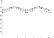
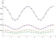
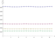
Figure 1: Total energy density and full power of the fields density for $\varphi^{2}_{a}$, $Z_{0a}^{2}$ (from the left to the right) fixing $\mu=1$, $\Omega=1$, varying $\alpha$ and $N$. $N=5$ (circle), $N=10$ (square), $N=15$ (triangle), $N=20$ (cross).

All tree graphs show an oscillating behavior of the values, this oscillation is present in all other quantities measured. The amplitude of this oscillation becomes smaller and smaller increasing the size of the matrix and this is true for all the quantities measured. The same trend is described in fig.2 in which position of the maximum are different but the amplitudes becomes smaller increasing $N$

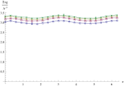
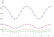
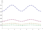
Figure 2: Total energy density and full power of the fields density for $\varphi^{2}_{a}$, $Z_{0a}^{2}$ (from the left to the right) fixing $\mu=1$, $\Omega=0.5$, varying $\alpha$ and $N$.

This results allow us to consider $\alpha=0$ for all next graphs, since we are interested in the behavior of the system for $N\to\infty$. This occurrence simplify all the next simulations thanks to the vanishing the of terms $\sim(\sin\alpha)/\Omega$ appearing in the discretized action. Beside, such results induce us to reckon the parameter $\alpha$ as connected to the remaining invariance of the vacuum state for the exact model.

8.2 Varying $\Omega$

Now we will analyze three cases in which $\mu$ is fixed to $0,1,3$, $\alpha$ is zero and we vary $\Omega\in[0,1]$. In the rest of this section we ignore for the computation of $E,D,V,F$ the prefactor $(1+\Omega^{2})$. In this way we focus our attention to the integral as the source of possible phase transitions. The graphs in fig.3 show the total energy density $\langle S\rangle/N^{2}$ and the various contributions: the potential $V/N^{2}$, the Yang-Mills part $F/N^{2}$ and the covariant derivative part $D/N^{2}$, for $\mu=1$. There is no evident discontinuity or peak and increasing the size of the matrices the curves remain smooth.

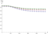
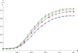
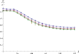
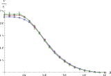
Figure 3: Total energy density and the various contributions for $\mu=1$, $\alpha=0$ varying $\Omega$ and $N$. From the left to the right $E$, $V$, $D$, $F$ with $N=5$ (circle), $N=10$ (square), $N=15$ (triangle), $N=20$ (cross).

Comparing the energy density and the various contributions fig.4 we notice that the contributions between $F$ and $V$ balance each other and the total energy follows the slope of $D$, this behavior continues increasing the size of the matrices fig.4.

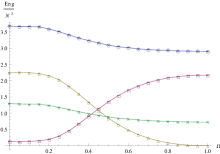
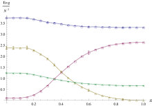
Figure 4: Comparison of the total energy density and the various contributions for $\mu=1$, $\alpha=0$. $E$ (circle), $F$ (triangle), $D$ (cross), $V$ (square). With $N=5$ (left) and $N=20$ (right).

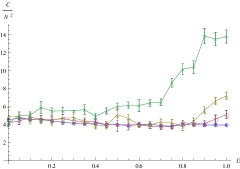
Figure 5: Specific heat for $\mu=1$.

The specific heat density shows fig.5 a peak in $\Omega=1$, this peak increases as $N$ increase. This behavior is typical of a phase transition, the peak is not clear for small $N$ due to the finite volume effect. In order to gain some informations on the composition of the fields we look at the order parameters defined in the previous chapter. Starting from $\psi$ field, in the figure 5 it is showed the graphs for $\varphi_{a}^{2}$, $\varphi^{2}_{0}$ and $\varphi^{2}_{1}$ for $N=5$.
The three values $\varphi_{a}^{2}$, $\varphi^{2}_{0}$ and $\varphi^{2}_{1}$ seem essentially constant, comparing the three graphs fig.6 it is easy to see the dominance of the spherical contribution $\varphi^{2}_{0}$ to the full power of the field.

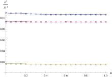
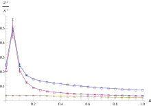
Figure 6: On the left comparison of $\varphi_{a}^{2}$ (circle), $\varphi^{2}_{0}$ (square) and $\varphi^{2}_{1}$ (triangle) density. On the right comparison of $Z_{0a}^{2}$ (circle), $Z_{00}^{2}$ (square) and $Z_{01}^{2}$ (triangle) density.

The behavior of the $Z_{0}$ fields is different, the spherical contribution becomes dominant approaching to $\Omega=0$ starting from a zone in which the contribution of $Z_{00}^{2}$ and $Z_{01}^{2}$ are comparable. For brevity will not be showed only the graphs for $Z_{0a}^{2}$, $Z_{00}^{2}$ and $Z_{01}^{2}$ but taking in account the statistical errors the other $Z_{i}$ related graphs appear compatible to the $Z_{0}$ case. The dependence of the previous quantities on $N$ are showed in the following graphs fig.7.

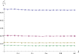
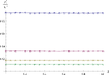
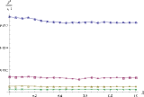
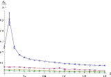
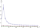
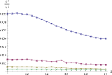
Figure 7: Starting from the up left corner and from the left to the right the densities for $\varphi_{a}^{2}$, $\varphi^{2}_{0}$, $\varphi^{2}_{1}$, $Z_{0a}^{2}$, $Z_{00}^{2}$ and $Z_{01}^{2}$ for $\mu=1$ varying $\Omega$ and $N$.

The values of the quantity of all the previous parameters decreases with $N$ but the dominance of the $\varphi_{0}$ on the total power of the field is independent by $N$. The peak related to $Z_{0}$ decrease, but if look at the single graph for $N=20$ the spherical contribution approaching the point $\Omega=0$ it features a peak.

Now we will analyze the model for $\mu=0$; fig.8 shows the graphs for total energy density and the contributions $V$, $D$, $F$. The slope of the total energy density seems to be constant. The $D$ contribution and the $F$ do not balance each other like in the previous case, but all the three contributions balance among them self to produce a constant sum.

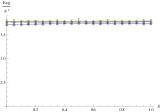
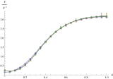
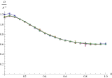
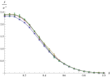
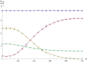
Figure 8: Total energy density, various contributions and the comparison among them for $\mu=0$ varying $\Omega$ and $N$. From the left to the right $E$, $V$, $D$, $F$ and comparison.

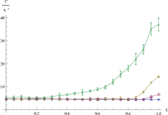
Figure 9: Specific heat density for $\mu=0$ varying $\Omega$ and $N$.

The specific heat density shows fig.9 again the peak in $\Omega=1$ as $N$ increase. For the other quantities $\varphi_{a}^{2}$, $\varphi^{2}_{0}$, $\varphi^{2}_{1}$ and $Z_{0a}^{2}$, $Z_{00}^{2}$, $Z_{01}^{2}$ we have the same behavior fig.12 of $\mu=1$ case, except for the oscillation appearing in the $Z_{0a}^{2}$, $Z_{00}^{2}$ graphs close to zero, anyway it appears only for $N=5$.

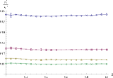
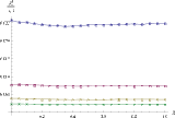
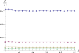
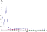
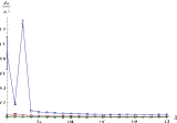
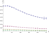
Figure 10: Starting from the up left corner and from the left to the right the densities for $\varphi_{a}^{2}$, $\varphi^{2}_{0}$, $\varphi^{2}_{1}$, $Z_{0a}^{2}$, $Z_{00}^{2}$ and $Z_{01}^{2}$ for $\mu=0$ varying $\Omega$ and $N$.

A complete different response of the system is described in the graphs for $\mu=3$, as we can see from fig.11. The slope of total energy density is very similar to the $F$ component instead $D$. Beside, appears a maximum around $\Omega=0.4$ for $N\to\infty$. This dramatic change of the graphs might be interpreted as consequence of a phase transition ruled by the parameter $\mu$, actually in the next section we will find a peak in the specific heat density for some fixed $\Omega$ and varying $\mu\in[0,3]$.

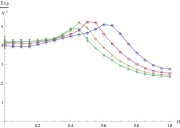
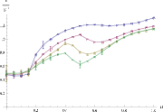
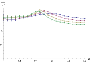
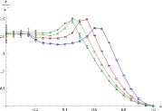
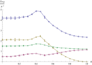
Figure 11: Total energy density, various contributions and the comparison among them for $\mu=3$ varying $\Omega$ and $N$. From the left to the right $E$, $V$, $D$, $F$ and comparison.

Specific heat density displays fig.12 a strong change too, in fact instead the peak in $\Omega=1$, it appears in the opposite side of the studied interval in $\Omega=0$. This peak too, due to its grows increasing $N$ could indicate a phase transition.

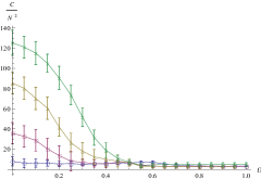
Figure 12: Specific heat density for $\mu=3$ varying $\Omega$ and $N$.

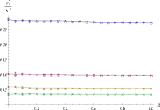
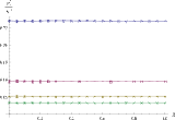
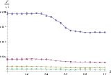
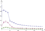
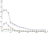
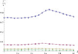
Figure 13: Starting from the up left corner and from the left to the right the densities for $\varphi_{a}^{2}$, $\varphi^{2}_{0}$, $\varphi^{2}_{1}$, $Z_{0a}^{2}$, $Z_{00}^{2}$ and $Z_{01}^{2}$ for $\mu=3$ varying $\Omega$ and $N$.

The fig.13 describes the behavior of the order parameters densities $\varphi_{a}^{2}$, $\varphi^{2}_{0}$, $\varphi^{2}_{1}$ and $Z_{0a}^{2}$, $Z_{00}^{2}$, $Z_{01}^{2}$, they have a similar aspect to the previous relative graphs. For the $\psi$ field the spherical contribution remains dominant, beside in the $\varphi^{2}_{1}$ graph appears a deviation from the constant slope this deviation is evident for $N=5$ but still there for higher $N$. The order parameters for $Z_{0}$ display a peak close to the origin without oscillations even for $N=5$. This maximum for higher $N$ does not move closer to the origin, in other words, this shift in not due to the finite volume effect. Even for $Z^{2}_{01}$ graph appears a deviation from the constant slope, a small peak which becomes shifted and smoother for higher $N$

8.3 Varying $\mu$

In this section is analyzed the response of the system varying $\mu\in[0,3]$ where $\Omega$ is fixed to $0,0.5,1$ and $\alpha$ is always zero. We start displaying the graphs fig.14 of the total energy density and of various contributions for $\Omega=0$. There is no evident discontinuity but appears a peak in the total energy density around $\mu\approx 2.5$ for $N=20$. Comparing all the contributions is easy to notice that the slope of the total energy is dictated by the curve $V$ of the potential part.

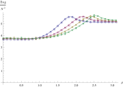
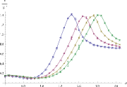
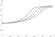
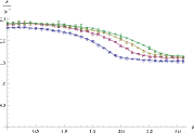
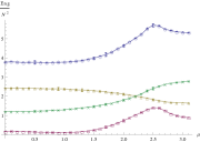
Figure 14: The total energy density and the various contributions for $\Omega=0$ varying $\mu$ and $N$. From the left to the right $E$, $V$, $D$, $F$ an comparison with $N=5$ (circle), $N=10$ (square), $N=15$ (triangle), $N=20$ (cross). For the comparison: $E$ (circle), $V$ (square), $D$ (triangle), $F$ (cross).

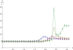
Figure 15: Specific heat density for $\Omega=0$ varying $\mu$ and $N$.

As mentioned before, the specific heat density fig.15 features a peak around $\mu\approx 2.5$ for $N=20$ and again, due to this behavior as $N$ increase, we could relate this peak to a phase transition. The plots for the quantities $\varphi_{a}^{2}$ and $\varphi^{2}_{0}$ denote a strong dependence on $\mu$, in particular the slope of $\varphi^{2}_{0}$ seems mostly linear, $\varphi^{2}_{1}$ related graphs feature a similar behavior but the slope is no longer linear. Comparing the three graphs fig.16 we deduce that close to the origin the non spherical contribution is bigger the spherical one, increasing $\mu$ this situation capsizes and $\varphi^{2}_{0}$ becomes dominant respect $\varphi^{2}_{1}$.

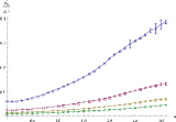
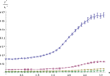
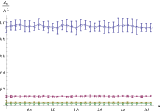
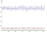
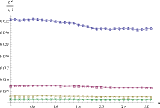
Figure 16: Starting from the up left corner and from the left to the right the densities for $\varphi_{a}^{2}$, $\varphi^{2}_{0}$, $\varphi^{2}_{1}$, $Z_{0a}^{2}$, $Z_{00}^{2}$ and $Z_{01}^{2}$ for $\Omega=0$ varying $\mu$ and $N$.

The behavior of the $Z_{0}$ fields is quite different, referring to figure 16, the spherical contribution is always dominant for the all interval $\mu\in[0,3]$. The curves for $Z_{0a}^{2}$, $Z_{00}^{2}$ are compatible to the constant slope, for $Z_{01}^{2}$ we have the same dependence on $\mu$ in particular there is a smooth descending step, however this step becomes smoother for bigger $N$. It is behooves to say that due to some cancellations effects the statistical errors are quite big and they can hide some dependence, anyway this results tell us about the dependence of the order parameter for $Z_{i}$ and in general of the system, on the two choice $\Omega=0$ or $\Omega\neq 0$.

Now we will analyze the model for $\Omega=0.5$; as fig.17 shows the graphs have a different slope comparing to the previous case, the maximum of total energy density follow the one of the $V$ component. If we focus ourself only on the total energy graph and we compare it with the one for $\Omega=0$, we notice a shift of the maximum for each $N$. In particular in fig.17 some maximum are moved outside the considered interval.

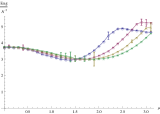
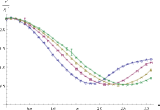
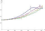
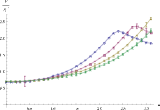
Figure 17: Total energy density and contributions for $\Omega=0.5$ varying $\mu$ and $N$. From the left to the right $E$, $V$, $D$, $F$.

We can find this shift very clearly looking at specific heat density graph fig.18, we find again the peak as $N$ increase but it is shifted around $\mu\approx 3.3$.

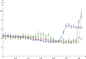
Figure 18: Specific heat density for $\Omega=0.5$ varying $\mu$ and $N$.

The graphs fig.21 for $\varphi_{a}^{2}$, $\varphi^{2}_{0}$ have the same behavior of $\Omega=0.5$ case, excluding some fluctuations close to the origin for $N=5$ due to the finite volume effect, $\varphi^{2}_{1}$ graph displays an almost constant curve. However, close to the origin, the spherical contribution and the first non spherical one are comparable.

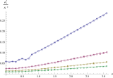
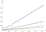
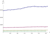
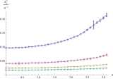
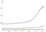
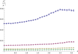
Figure 19: Starting from the up left corner and from the left to the right the densities for $\varphi_{a}^{2}$, $\varphi^{2}_{0}$, $\varphi^{2}_{1}$, $Z_{0a}^{2}$, $Z_{00}^{2}$ and $Z_{01}^{2}$ for $\Omega=0.5$ varying $\mu$ and $N$.

The introduction of $\Omega\neq 0$ creates, in the $Z_{0}$ fields order parameters fig.19, a dependence similar to the graphs for the $\psi$; the full power of the field density and the spherical contribution are no more constant and they grow increasing $\mu$. Even in this case the spherical contribution is always dominant excluding the region around $\mu=0$.

The last set of graphs for the 4-dimensional model are obtained fixing $\Omega=1$, due to the vanishing of prefactor in front of the Yang-Mills part of the action the $F$ contribution is always zero. The following diagrams for the energy and contributions show the absence of the previous peak and comparing again them with former graphs they seem a sort dilatation.

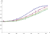
Figure 20: Total energy density and the various contributions for $\Omega=1$ varying $\mu$ and $N$. From the left to the right $E$, $V$, $D$.

The specific heat density does not show the peak in zero any more fig.21 and the curves does not show any particular point as $N$ increase, actually the peak can be found for higher $\mu$.

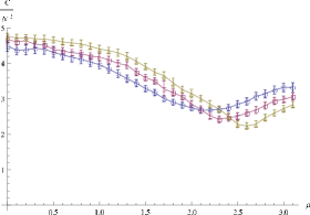
Figure 21: Specific heat density for $\Omega=1$ varying $\mu$ and $N$.

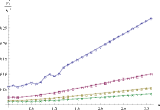
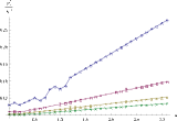
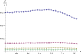
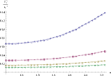
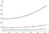
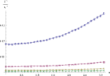
Figure 22: Starting from the up left corner and from the left to the right the densities for $\varphi_{a}^{2}$, $\varphi^{2}_{0}$, $\varphi^{2}_{1}$, $Z_{0a}^{2}$, $Z_{00}^{2}$ and $Z_{01}^{2}$ for $\Omega=1$ varying $\mu$ and $N$.

At last in fig.22 we found a behavior of the order parameters density for $Z_{0}$ and $\psi$ fields similar to the former graphs for $\Omega=0.5$ and they are compatible with a dilatation of the previous diagrams.

Conclusions and prospectives

We have presented a study of a spectral action model constructed in order to extend to the Yang-Mills theories the non-commutative Wulkenhaar-Grosse model. The main aim of this work was to test a first Monte Carlo approach based on a non-perturbative regularization method. We have performed Monte Carlo simulations and obtained the values of the defined observables varying the parameters of the system. Despite the complexity of the approximated spectral action considered here we were able to obtain some reliable numerical results, we can conclude that a numerical approach of this kind of model using the matrix Moyal base seems feasible. The specific heat density shows various peaks indicating phase transitions, in particular studying the behaviors for some fixed $\mu$ we found a peak around $\Omega=0$ for $\mu=\{0,1\}$ and peak in $\Omega=1$ for $\mu=3$, beside we notice a huge change in the energy density and in its contributions between the cases $\mu=\{0,1\}$ and $\mu=3$. Other peaks in the specific heat density can be found varying $\mu$ and fixing $\Omega$, the graphs show that increasing $\Omega$ the peak in the specific heat, starting from $\mu\approx 2.4$ for $\Omega=0$, is moved towards higher $\mu$. The order parameters introduced show a strong dependence on the occurrence of $\Omega=0$ or $\Omega\neq 0$. Referring to the fixed $\mu$ graphs we found a peak in the spherical contribution for the gauge fields $Z_{i}$, we can interpreted this slope as a sort of symmetry breaking introduced by $\Omega\neq 0$. Additionally, varying $\mu$ and fixing $\Omega$ the other parameters display an increasing slope with $\mu$ for all fields and all situation but one; the graphs of the order parameters concerning $Z_{0a}$, $Z_{00}$ for $\Omega=0$ show a constant behavior. The natural next steps in the numerical study of this model, could be the computation of the transition curves in order to separate the phase regions and classify them using eventually some additional order parameters. Our treatment, forced by limited resource, was conducted conjecturing that the system can fully described varying $\Omega$ in the range $[0,1]$ but since the L-S duality does not hold any more in our case, will be very useful to extend this range. Actually, the computed graphs does not show any periodicity in $\Omega\in[0,1]$ so there are some hints to infer that the range $[0,1]$ is not enough, however only a direct computation will clarify this point. Will be very interesting to do not require any more the condition $\mu^{2}>0$, in order to implement this change we have to conduct the calculation no more around the minimum of the actions. The expansion of the parameters space, together with the classification of the different phase regions allows us to compare our model with the results of the simulation conducted on the fuzzy spaces, looking in particular about the occurrence of the so called non-uniformly ordered phase which is connected with the UV/IR mixing. Since we have constructed our model starting from a renormalizable one this study is very desirable.

References

- [1] A. Connes, Noncommutative Geometry, Academic Press, Inc. (1994).
- [2] A. Connes, Geometry from the spectral point of view, Lett. Math. Phys. 34 (1995), no. 3, 203–238.
-
[3]
A. Connes, On the spectral characterization of manifolds,
(2008) arXiv:0810.2088v1[math.OA]. - [4] A. Connes, Noncommutative geometry and reality, J. Math. Phys. 36 (1995) 6194.
- [5] V. Gayral, J. H. Jureit, T. Krajewski and R. Wulkenhaar, Quantum field theory on projectivemodules, CPT-P67-2006 [hep-th/0612048].
- [6] A. Connes, Gravity coupled with matter and the foundation of noncommutative geometry, Comm. Math. Phys. 155 (1996) 109.
- [7] A. Rennie Joseph and C. Varilly Reconstruction of manifolds in noncommutative geometry, (2006) arXiv:math/0610418v4[math.OA].
- [8] M.R. Douglas, D-Geometry and Noncommutative Geometry, [hep-th/9901146].
- [9] C.P. Martin and D. Sanchez-Ruiz, The One-loop UV Divergent Structure of U(1) Yang-Mills Theory on Noncommutative , Phys.Rev.Lett. 83 (1999) 476-479, [hep-th/9903077].
- [10] A. Connes and J. Lott, Particle models and noncommutative geometry (expanded version), Nucl. Phys. Proc. Suppl. 18B (1991) 29.
- [11] A. Matusis, L. Susskind and N. Toumbas, The IR/UV connection in the non-commutative gauge theories, JHEP 0012 (2000) 002 [arXiv:hep-th/0002075].
- [12] I. Chepelev, R. Roiban,Convergence theorem for non-commutative Feynman graphs and renormalization, JHEP 0103 (2001) 001 [arXiv:hep-th/0008090].
- [13] T. Krajewski, R. Wulkenhaar,Perturbative quantum gauge fields on the noncommutative torus, [hep-th/9903187].
- [14] V. Rivasseau, F. Vignes-Tourneret, R. Wulkenhaar, Renormalization of non-commutative -theory by multi-scale analysis, Phys. Lett. B533 (2002) 168–177, [hep-th/0202039].
- [15] V. Rivasseau, Constructive Matrix Theory, arXiv:0706.1224 [hep-th].
- [16] R. Gurau and V. Rivasseau, Parametric representation of noncommutative field theory,Commun. Math. Phys. 272 (2007) 811 [arXiv:math-ph/0606030].
- [17] V. Gayral, B. Iochum, The spectral action for Moyal planes, J. Math. Phys. 46 (2005). 043503 [arXiv:hep-th/0402147].
- [18] H. Grosse and R. Wulkenhaar, -spectral triple on -Moyal space and the vacuum of noncommutative gauge theory, arXiv:0709.0095[hep-ht].
- [19] V. Gayral and R. Wulkenhaar In preparation.
- [20] A. de Goursac, J.-C. Wallet, and R. Wulkenhaar, On the vacuum states for noncommutative gauge theory, Eur. Phys. J. C56 (2008) 293–304,arXiv:0803.3035 [hep-th].
- [21] I. Montvay and G. Münster, Quantum Field Theory on a Lattice, Cambridge University Press, (1997).
- [22] M. E. Newman and G. T. Barkema,Monte Carlo Methods in Statistical PhysicsOxford University Press (2002).
- [23] H. Chamseddine and A. Connes, The Spectral Action Principle, Math.Phys.186:731-750 (1997).
- [24] H. Grosse and R. Wulkenhaar, Renormalisation of -theory on noncommutative in the matrix base, Commun. Math. Phys. 256 (2005) 305 [arXiv:hep-th/0401128].
- [25] H. Grosse and R. Wulkenhaar, Power-counting theorem for non-local matrix models and renormalisation, [arXiv:hep-th/0305066].
- [26] V. Gayral, J. M. Gracia-Bondia. Iochum, T. Schücker and J. C. Varilly, Moyal planes are spectral triples, Commun. Math. Phys. 246 (2004) 569 [arXiv:hep-th/0307241].
- [27] V. Gayral, J. M. Gracia-Bondia and F. Ruiz, Position-dependent noncommutative products: Classical construction and field theory, Nucl. Phys. B 727 (2005) 513 [arXiv:hep-th/0504022].
- [28] J.M. Gracia-Bondia, J.C. Varilly, H. Figueroa, Algebras of distributions suitable for phase-space quantum mechanics, I, J. Math. Phys. 29, (1988).
- [29] X. Martin, A matrix phase for the scalar field on the fuzzy sphere, JHEP 0404 (2004) 077 [hep-th/0402230].
- [30] J. Medina, Fuzzy Scalar Field Theories: Numerical and Analytical Investigations, arXiv:0801.1284v1 [hep-th].
- [31] I. Gradshteyn and I. M. Ryzhik, Table of integrals, series, and products, Academic Press, San Diego, 6th ed., (2000).
- [32] E. Langmann and R. J. Szabo, Duality in scalar field theory on noncommutative phase spaces, Phys. Lett. B533 (2002) 168–177, [hep-th/0202039].