Diffusion and Relaxation Controlled by Tempered $\alpha$-stable Processes

Abstract

We derive general properties of anomalous diffusion and nonexponential relaxation from the theory of tempered $\alpha$-stable processes. Its most important application is to overcome the infinite-moment difficulty for the $\alpha$-stable random operational time $\tau$. The tempering results in the existence of all moments of $\tau$. The subordination by the inverse tempered $\alpha$-stable process provides diffusion (relaxation) that occupies an intermediate place between subdiffusion (Cole-Cole law) and normal diffusion (exponential law). Here we obtain explicitly the Fokker-Planck equation, the mean square displacement and the relaxation function. This model includes subdiffusion as a particular case.

Introduction.— Many studies have been reported on the phenomenon of subdiffusion which is typically observed when, due to dominating influence of traps (see Metzler and Klafter (2000); Zaslavsky (2002); Sokolov and Klafter (2006) and reference therein), the waiting times of random walks become $\alpha$-stable, $\alpha<1,$ with an infinite mean. However, this picture is only an idealization of the physical world. In reality the time of trap life can be restricted. It should be taken into account that the traps can be located in some spatial regions from which a walker may easily escape. Consequently, in a more general representation, the random walks start as subdiffusion, but their characteristics become very similar to those of normal diffusion at large time scales. One of such clear examples is a random motion of bright points (BP) associated with magnetic fields at the solar photosphere. The BP transport in the intergranular lanes with times less than 20 minutes has a subdiffusive character, but the analysis of the BP motion supports the normal diffusion behavior for larger times. The experimental result is reported in Cadavid et al. (1999). The present paper is just devoted to such a problem. For this purpose we are going to apply the tempered $\alpha$-stable processes for the description of diffusion and relaxation. In comparison with the purely $\alpha$-stable process such a process has finite moments, but it saves some important rudiments of the stable process too Rosiński (2007); Piryatinska et al. (2005); Terdik and Woyczynski (2006). Therefore, if its inverse process is taken as a subordinator, it provides then a diffusive picture occupying an intermediate place between subdiffusion and normal diffusion.

Tempered $\alpha$-stable process and its inverse.— The model of subdiffusion is based on a flexible Montroll-Weiss idea on continuous time random walks (CTRW) Montroll and Weiss (1965). Briefly, the representation of anomalous diffusion by means of the CTRW methodology is the following (for more details see, for example, Stanislavsky (2004); Magdziarz and Weron (2006)). Consider a sequence ${T_{i}}$, $i=1,2,\dots$ of non-negative, independent, identically distributed (iid) random variables which represent waiting-time intervals between subsequent jumps of a walker. The random time interval of $n$ jumps in space equals $T(n)=\sum_{i=1}^{n}T_{i}$ with $T(0)$ = 0. The random number $N_{t}$ of jumps, performed by the walker up to time $t>0$, is determined by the largest index $n$ for which the sum of $n$ interjump time intervals does not exceed the observation time $t$, namely $N_{t}=\max\{n:T(n)\leq t\}$. The position of the walker after $N_{t}$ jumps becomes then

$$R(N_{t})=\sum_{i=1}^{N_{t}}R_{i},$$ (1)

where $R_{i}$ are iid variables giving both the length and the direction of the i-th jump. The process (1) is just known as the CTRW.

If the time intervals $T_{i}$ belong to the domain of attraction of a completely asymmetric $\alpha$-stable distribution with the index $0<\alpha<1$, the generalization of the central limit theorem yields the continuous limit $a^{-1/\alpha}T([a\tau])\stackrel{{\scriptstyle d}}{{\rightarrow}}U_{\tau}$ as $a\to\infty$, where $U_{\tau}$ is a strictly increasing $\alpha$-stable L$\acute{\rm e}$vy process, $a>0$ parameter, $[x]$ denotes the integer part of $x$ and “$\stackrel{{\scriptstyle d}}{{\rightarrow}}$” means “tends in distribution”. Similarly, let the jumps $R_{i}$ belong to the domain of attraction of a $\gamma$-stable distribution $S_{\gamma,\beta}(x),0<\gamma\leq 2,|\beta|\leq 1$ so that $a^{-1/\gamma}R([a\tau])\stackrel{{\scriptstyle d}}{{\rightarrow}}X_{\tau}$ as $a\to\infty$, where $X_{\tau}$ is a $\gamma$-stable L$\acute{\rm e}$vy process known as the parent process. If $\gamma=2$, the parent process is the classical Brownian motion. Both, the process $U_{\tau}$ and the process $X_{\tau}$ are indexed by random operational (internal) time $\tau$. In order to find a particle position at the observable time $t$, we have to introduce the notion of the inverse-time $\alpha$-stable subordinator $S_{t}$ relating the internal and the observable times

$$a^{-\alpha}N_{at}\stackrel{{\scriptstyle d}}{{\rightarrow}}S_{t}=\inf\{\tau:U_{\tau}>t\}\qquad$$ (2)

as $a\to\infty$. Then, as $a\to\infty$, the continuous limit of the CTRW process (1) obtains the following form

$$a^{-\alpha/\gamma}R(N_{at})\approx(a^{\alpha})^{-1/\gamma}R([a^{\alpha}S_{t}])\stackrel{{\scriptstyle d}}{{\rightarrow}}X(S_{t}),$$ (3)

known as the anomalous diffusion process Meerschaert et al. (2002), directed by the inverse $\alpha$-stable subordinator $S_{t}$. It should be pointed out that the process $U_{\tau}$ does not have any finite $p$-moments for $p\leq\alpha$. Therefore, the subdiffusion is characterized by a power mean square displacement in time Stanislavsky (2004); Magdziarz and Weron (2006); Stanislavsky (2003).

However, there are physical phenomena, for example, the random motion of BPs in intergranular lanes on the Sun, where it would be desirable to get also a model that overcomes the infinite-moment difficulty while preserving the subdiffusive behavior for short times Stanislavsky and Weron (2007). The remedy was first proposed in the physical literature by Mantegna and Stanley Mantegna and Stanley (1994). Their idea of truncated Lévy flights served as a model for random phenomena which exhibit at small scales properties similar to those of Lévy flights, but have distributions which at large scales have cutoffs and thus have finite moments of any order. Koponen Koponen (1995), building on Mantegna and Stanley’s ideas, defined the smoothly truncated Lévy flights which stressed the advantage of a nice analytic form. Independently, the same family of distributions was described earlier by Hougaard Hougaard (1986) in the context of a biological application. However, different methods for the truncation were suggested also in the economic and statistical sciences Boyarchenko and Levendorskij (2002); Carr et al. (2002); Kim et al. (2008), but until the Rosiński’s paper Rosiński (2007) there was a lack of invariance under linear transformations for the distributions introduced, a significant property that the $\alpha$-stable laws possess. He succeeded in finding the appropriate class of tempered stable distributions and processes Terdik and Woyczynski (2006); Kim et al. (2008).

In what follows we discuss properties of a diffusion process which is related to an inverse tempered $\alpha$-stable subordinator. The Laplace image for the probability density function (p.d.f.) of a tempered non-negative $\alpha$-stable variable is

$$\tilde{f}(u)=\exp\left(\delta^{\alpha}-(u+\delta)^{\alpha}\right)\,,$$ (4)

where $\delta$ is a positive constant and $0<\alpha<1$ Piryatinska et al. (2005). If $\delta$ equals zero, the tempered $\alpha$-stable p.d.f. becomes simply $\alpha$-stable. Eq.(4) describes probabilistic properties of the tempered $\alpha$-stable Lévy process $U(\tau)$ which generalizes the above mentioned process $U_{\tau}$.

Next, we will find its inverse process $S(t)$ as in (2), where $U(\tau)$ substitutes $U_{\tau}$. If $f(t,\tau)$ is the p.d.f. of $U(\tau)$, then the p.d.f. $g(\tau,t)$ of its inverse $S(t)$ can be represented as

$$g(\tau,t)=-\frac{\partial}{\partial\tau}\int_{-\infty}^{t}f(t^{\prime},\tau)\,dt^{\prime}.$$

Taking the Laplace transform of $g(\tau,t)$ with respect to $t$, we get

$$\tilde{g}(\tau,u)=\frac{(u+\delta)^{\alpha}-\delta^{\alpha}}{u}\,e^{-\tau[(u+\delta)^{\alpha}-\delta^{\alpha}]}\,.$$ (5)

When $u\gg 1$ ($t\ll 1$) or $\delta\to 0$, Eq. (5) tends to

$$\tilde{g}(\tau,u)=u^{\alpha-1}\,e^{-\tau u^{\alpha}}\,,$$ (6)

which is the Laplace image of an inverse $\alpha$-stable p.d.f. typical for subdiffusion. If $u\ll 1$ ($t\gg 1$) or $\alpha\to 1$, then Eq. (5) becomes the Laplace image of the Dirac delta-function. It follows from Eq. (6) that the p.d.f. of the inverse $\alpha$-stable process is

$$g(\tau,t)=\frac{1}{2\pi i}\int_{Br}e^{ut-\tau u^{\alpha}}\,u^{\alpha-1}\,du=t^{-\alpha}F_{\alpha}(\tau/t^{\alpha})\,,$$

where $Br$ denotes the Bromwich path, and the function $F_{\alpha}(z)$ is a specific case of the Wright function Erdélyi (1955); Stanislavsky (2004).

Subordination by an inverse tempered $\alpha$-stable process.— Let the parent process $X(\tau)$ have the p.d.f. $h(x,\tau)$. Then the p.d.f. of the subordinated process $X[S(t)]$ obeys the integral relationship between the pro-bability densities of the parent and directing processes, $X(\tau)$ and $S(t)$, respectively,

$$p(x,t)=\int^{\infty}_{0}h(x,\tau)\,g(\tau,t)\,d\tau.$$ (7)

In the Laplace space the probability density $p(x,t)$ has the most simple form. Taking into account Eq. (5), the Laplace transform of Eq. (7) with respect to $t$ gives

$$\tilde{p}(x,u)=\frac{(u+\delta)^{\alpha}-\delta^{\alpha}}{u}\,\tilde{h}(x,(u+\delta)^{\alpha}-\delta^{\alpha}).$$ (8)

For $\delta=0$ the latter expression becomes $u^{\alpha-1}\tilde{h}(x,u^{\alpha})$.

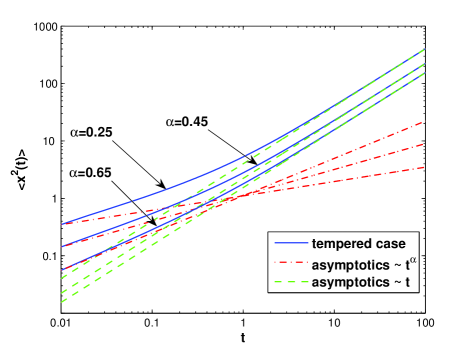
Figure 1: (Color online) Mean square displacement of anomalous diffusion subordinated by an inverse tempered $\alpha$-stable process.

It is not difficult to calculate the moments of the process $X[S(t)]$ if the moments of the process $X(\tau)$ are known. For example, for the Gaussian process ($\gamma=2$) the second moment is $\left\langle X^{2}(\tau)\right\rangle=D\tau$, where $D$ is a diffusive constant. Then the mean square displacement of $X[S(t)]$ can be written as

$$\left\langle X^{2}[S(t)]\right\rangle=\int^{\infty}_{0}\left\langle X^{2}(\tau)\right\rangle\,g(\tau,t)\,d\tau\,.$$

The Laplace image $\tilde{\left\langle X_{u}^{2}\right\rangle}$ of $\left\langle X^{2}[S(t)]\right\rangle$ has the form

$$\tilde{\left\langle X_{u}^{2}\right\rangle}=\frac{D}{u[(u+\delta)^{\alpha}-\delta^{\alpha}]}\,.$$ (9)

Consequently, the inverse Laplace transform of Eq. (9) reads

$$\frac{1}{u[(u+\delta)^{\alpha}-\delta^{\alpha}]}\stackrel{{\scriptstyle{\cal L}^{-1}}}{{\rightarrow}}\int_{0}^{t}e^{-\delta y}\,y^{\alpha-1}\,E_{\alpha,\,\alpha}(\delta^{\alpha}y^{\alpha})\,dy\,,$$ (10)

where

$$E_{\alpha,\,\beta}(z)=\sum_{k=0}^{\infty}\frac{z^{k}}{\Gamma(\alpha k+\beta)},\quad\alpha>0,\quad\beta>0$$

is the Mittag-Leffler function Erdélyi (1955). The function (10) gives rise to interesting asymptotic properties of the mean square displacement $\left\langle X^{2}[S(t)]\right\rangle$. For $t\ll 1$ this displacement behaves as $Dt^{\alpha}/\Gamma(\alpha+1)$, but for $t\gg 1$ it increases linearly in time $Dt/\alpha$ (see Fig. 1). Thus the anomalous diffusion, governed by the inverse tempered $\alpha$-stable subordinator, occupies an intermediate place between sub-diffusion and the normal diffusion. For short times it behaves as subdiffusion whereas for the long times it resembles the properties of the normal diffusion. Let us call the diffusion subordinated by the inverse tempered $\alpha$-stable process as a “tempered subdiffusion”. As is well known Baeumer et al. (2005), the inverse $\alpha$-stable process accounts for the amount of time, when a walker does not participate in a motion. By analogy, we may conclude that the process $S(t)$ for the tempered subdiffusion represents a case, when a walker does not participate in a motion only for restricted intervals of time. At large time scales the walker begins to move randomly without any stopping as if $\alpha=1$.

Equation of tempered subdiffusion.— Let $\hat{L}(x)$ be a time-independent Fokker-Planck operator (FPE), whose exact form is not important here. Let the ordinary FPE $\partial h(x,\tau)/\partial\tau=\hat{L}(x)\,h(x,\tau)$ describe the evolution of a particle subject to the operation time $\tau$. Acting by the operator $\hat{L}(x)$ on the image $\tilde{p}(x,u)$ from Eq. (8), we find

$$\hat{L}(x)\,\tilde{p}(u,x) = [(u+\delta)^{\alpha}-\delta^{\alpha}]\,\tilde{p}(x,u)-$$ (11)

$$- q(x)\,\frac{[(u+\delta)^{\alpha}-\delta^{\alpha}]}{u}\,,$$

where $q(x)$ is an initial condition. When $\delta=0$, the inverse Laplace transform of the latter expression gives a fractional representation of the FPE Metzler and Klafter (2000); Stanislavsky (2004)

$$p(x,t) = q(x)+$$ (12)

$$+ \frac{1}{\Gamma(\alpha)}\int_{0}^{t}d\tau\,(t-\tau)^{\alpha-1}\,\hat{L}(x)\,p(x,\tau)\,.$$

In the case of the tempered subdiffusion the kernel in the integral representation of the FPE will be more complex, containing as a special case the kernel of Eq.(12) for $\delta\to 0$. Using the formal integral representation of the FPE

$$p(x,t)=q(x)+\int_{0}^{t}d\tau\,M(t-\tau)\,\hat{L}(x)\,p(x,\tau)\,.$$ (13)

and taking the inverse Laplace transform of Eq.(11), we obtain the explicit form of the kernel $M(t)$, namely

$$M(t)=e^{-\delta t}\,t^{\alpha-1}\,E_{\alpha,\,\alpha}(\delta^{\alpha}t^{\alpha})\,.$$ (14)

For $t\ll 1$ (or $\delta\to 0$) this function takes the power form $t^{\alpha}/\Gamma(\alpha)$ as the kernel in Eq. (12). However, for $t\gg 1$ (or $\alpha\to 1$) $M(t)$ becomes constant and, as a result, Eq. (13) transforms into the integral form of the ordinary FPE.

Tempered relaxation.—The commonly accepted theoretical approaches to model relaxation phenomena assume Metzler and Klafter (2000) decay of an excitation undergoing diffusion in the system under consideration. In this framework, the relaxation function $\phi(t)$ describes the temporal decay of a given mode $k$ and can be expressed Magdziarz and Weron (2006) through the Fourier transform of the diffusion process $X[S(t)]$

$$\phi(t)=\left\langle e^{-kX[S(t)]}\right\rangle\,.$$ (15)

Here $k>0$ has the physical meaning of a wave number (the Fourier image of spatial coordinates). Starting with Eq. (5), we can write the Laplace image of Eq. (15) as

$$\tilde{\phi}(u)=\frac{[(u+\delta)^{\alpha}-\delta^{\alpha}]}{u[\Phi(k)+(u+\delta)^{\alpha}-\delta^{\alpha}]}\,,$$ (16)

where $\Phi(k)$ is the logarithm of the characteristic function of the process $X(\tau)$.

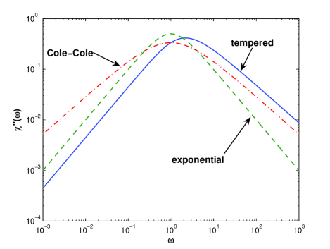
Figure 2: (Color online) Absorption (imaginary) term of the frequency-domain relaxation function $\chi(\omega)=\chi^{\prime}(\omega)-i\chi^{\prime\prime}(\omega)$ for $\alpha$ = 0.75 .

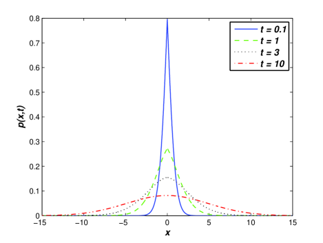
Figure 3: (Color online) Propagator $p(x,t)$ for the tempered diffusion with $\alpha$ = 2/3 and $\delta$ = 0.5, drawn for consecutive dimensionless instances of time $t$ = 0.1, 1, 3, 10. The cusp shape of the p.d.f. disappears.

To expose the characteristic properties of the “tempered relaxation” we use the frequency-domain description Jonscher (1996); Jurlewicz (2005) of the relaxation phenonenon

$$\chi(\omega)=\int^{\infty}_{0}e^{-i\omega t}\,\left(-\frac{d\phi(t)}{dt}\right)\,dt\,.$$ (17)

Then, for the relaxation under the inverse tempered $\alpha$-stable process the function (17) takes the form

$$\chi(\omega)=\frac{1}{1-\sigma^{\alpha}+(i\omega/\omega_{p}+\sigma)^{\alpha}}\,,$$ (18)

where $0\leq\sigma\leq 1$ is a constant, and $\omega_{p}$ is the characteristic frequency of the relaxing system.

According to Eq. (18), for $\sigma=0$ the relaxation function describes the Cole-Cole law. If $\alpha=1$, the function becomes exponential. In the case of $\sigma=1$ it has the Cole-Davidson form. The relaxation directed by the inverse tempered $\alpha$-stable process takes an intermediate place between the superslow relaxation and the exponential one (see Fig. 2). Such a type of evolution is observed in relaxation experiments (see, for example, Jonscher (1996)).

Conclusions.— In summary we have developed a novel approach to anomalous diffusion and nonexponential relaxation from tempered $\alpha$-stable processes. The model is broader than the purely subdiffusive case. It is very important that they both can be considered on the unique base following the theory of subordinated random processes. We have derived a tempered form of the FPE and the relaxation function, as well as we have calculated the mean square displacement describing the processes. In Fig. 3, as an example, the propagator $p(x,t)$ for the tempered diffusion with $\alpha$ = 2/3 and $\delta$ = 0.5, is drawn. The cusp shape of the p.d.f. disappears when time increases. Thus our model occupies an intermediate place between subdiffusion and normal diffusion. We expect that our results will yield insights into the coexistence of subdiffusion and normal diffusion in nature.

AS is grateful to the Institute of Physics, Wrocław University of Technology for kind hospitality during his visit.

References

- Metzler and Klafter (2000) R. Metzler, E. Barkai, and J. Klafter, Phys. Rev. Lett. 82, 3563 (1999); R. Metzler and J. Klafter, Phys. Rep. 339, 1 (2000).
- Zaslavsky (2002) G.M. Zaslavsky, Phys. Rep. 371, 461 (2002).
- Sokolov and Klafter (2006) I.M. Sokolov and J. Klafter, Phys. Rev. Lett. 97, 140602 (2006).
- Cadavid et al. (1999) A.C. Cadavid, J.K. Lawrence, and A.A. Ruzmaikin, Astrophys. J. 521, 844 (1999).
- Rosiński (2007) J. Rosiński, Stoch. Proc. Appl. 117, 677 (2007).
- Piryatinska et al. (2005) A. Piryatinska, A.I. Saichev, and W.A. Woyczynski, Physica A 349, 375 (2005).
- Terdik and Woyczynski (2006) G. Terdik and W.A. Woyczynski, Prob. Math. Statist. 26, 213 (2006).
- Montroll and Weiss (1965) E.W. Montroll and G.H. Weiss, J. of Math. Phys. 6, 167 (1965); H. Scher and E.W. Montroll, Phys. Rev. B 12, 2455 (1975); M. Shlesinger, J. Stat. Phys. 10, 421 (1974).
- Stanislavsky (2004) A.A. Stanislavsky, Theor. Math. Phys. 138, 418 (2004).
- Magdziarz and Weron (2006) M. Magdziarz and K. Weron, Physica A 367, 1 (2006).
- Meerschaert et al. (2002) M.M. Meerschaert, D.A. Benson, H.P. Scheffler, and B. Baeumer, Phys. Rev. E 65, 041103 (2002).
- Stanislavsky (2003) A.A. Stanislavsky, Phys. Rev. E 67, 021111 (2003).
- Stanislavsky and Weron (2007) A.A. Stanislavsky and K. Weron, Astrophys. Space Sci. 312, 343 (2007).
- Mantegna and Stanley (1994) R.N. Mantegna and H.E. Stanley, Phys. Rev. Lett. 73, 2946 (1994).
- Koponen (1995) I. Koponen, Phys. Rev. E 52, 1197 (1995).
- Hougaard (1986) P. Hougaard, Biometrica 73(2), 387 (1986).
- Boyarchenko and Levendorskij (2002) S.J. Boyarchenko and S.Z. Levendorskij, Int. J. Theor. Appl. Finance 3, 549 (2002).
- Carr et al. (2002) P. Carr, H. Geman, D. Madan, and M. Yor, J. Business 75, 305 (2002).
- Kim et al. (2008) Y.S. Kim, S.T. Rachev, D.M. Chung, and M.L. Bianchi, Prob. Math. Statist. 28, 168 (2008).
- Erdélyi (1955) A. Erdélyi, Higher Transcendental Functions, Vol III (McGraw-Hill, New York, 1955).
- Baeumer et al. (2005) B. Baeumer, D.A. Benson, and M.M. Meerschaert, Physica A 350, 245 (2005).
- Jonscher (1996) A.K. Jonscher, Universal Relaxation Law (Chelsea Dielectrics Press, London, 1996).
- Jurlewicz (2005) A. Jurlewicz, Dissertationes Math. 431, 1 (2005).