Hamiltonian formalism of fractional systems

Abstract

In this paper we consider a generalized classical mechanics with fractional derivatives. The generalization is based on the time-clock randomization of momenta and coordinates taken from the conventional phase space. The fractional equations of motion are derived using the Hamiltonian formalism. The approach is illustrated with a simple-fractional oscillator in a free state and under an external force. Besides the behavior of the coupled fractional oscillators is analyzed. The natural extension of this approach to continuous systems is stated. The interpretation of the mechanics is discussed.

1 Introduction

The fractional differential equations become very popular for describing anomalous transport, diffusion-reaction processes, superslow relaxation, etc 1 ; 2 ; 2a ; 3 (and the references therein). The interest is stimulated by the applications in various areas of physics, chemistry and engineering 3a ; 4 ; 5 ; 5a ; 6 ; 6a ; 6b . Nevertheless, the derivation of such equations from some first physical principles is not an easy matter. The fractional operator reflects intrinsic dissipative processes that are sufficiently complicated in nature. Their theoretical relationship with fractional calculus is not yet ascertained in full.

The classical Hamiltonian (or Lagrangian) mechanics is formulated in terms of derivatives of integer order. This technique suggests advanced methods for the analysis of conservative systems, while the physical world is rather nonconservative because of friction. The account of frictional forces in physical models increases the complexity in the mathematics needed to deal with them.

The fractional Hamiltonian (and Lagrangian) equations of motion for the nonconservative systems were introduced into consideration by Riewe 7 . His approach is based on a simple look-out. If the frictional force is proportional to velocity, the functional form of a classical Lagrangian without friction may be added by a term with the fractional derivative of one-half order. After applying the variational technique, the obtained equation of motion for the nonconservative system contains a contribution of the frictional force. An extension of the fractional variational problem for constrained systems was offered in 7a ; 7b . However, as it was observed by Dreisigmeyer and Young 8 , the conception conflicts with the principle of causality. The point is that the variational principle utilizes the integration by part. After this operation the left Riemann-Louville fractional derivative transforms into the right one which has a reversal arrow of time. Unfortunately, the attempt to overcome this problem by means of the treatment of the action as a Volterra series was unsuccessful 8a .

An alternative approach for determining the fractional equations of motion has been developed recently in 9 . They are derived by means of the fractional normalization condition. This condition can be considered as a normalization condition for the distribution function in a fractional space. The volume element of the fractional phase space is realized by fractional exterior derivatives. In this case the fractional system is described by a fractional power of coordinates and momenta. Therefore, such fractional systems are essentially nonlinear.

The purpose of the present paper is to provide a general method for describing the fractional systems from some first principles. We will look at the problem from another point of view. The main difference of our consideration from above is a deep interrelation of the fractional temporal derivative with stable distributions from the theory of probability. Also, we intend to investigate some concrete physical applications. Our paper is organized as follows. The appearance of the fractional derivative in the equations of motion is conditioned on a peculiar interaction of a physical system with environment. In Sect. 2 it is shown that the interaction is taken into account through the temporal variable that represents a sum of random intervals identically distributed. The probability distribution of such a sum asymptotically tends to a stable distribution. Using this approach we derive the equation of motion in Sect. 3. Based on the derivation the next section is devoted to the fractional oscillator. The effect of the fractional damping on resonance is considered in Sect. 5. This feature is similar to an exponential damping, but there are some differences. Further the dynamics of coupled fractional oscillators is represented in Sect. 6. The forced oscillations of a multiple fractional system are analyzed in Sect. 7. The generalization of discrete fractional systems on a continuous case is suggested in Sect. 8. In conclusion we discuss an interpretation of the fractional mechanics.

2 Operational time and subordination

The spacetime is often treated as a continuum. It is something like an ideal elastic medium. The conjecture is the overarching principle of all physics. However, the concept is a fiction. Nowhere does this feature of spacetime show itself more clearly than at big bang and at collapse that it cannot be a continuum. The “elasticity” of spacetime is only an approximation. There are very different viewpoints to the space-time problem. One hopes that an appropriate model for spacetime will be built in some satisfactory theory of quantum gravitation. Others opt for some type of discrete structures abandoning a continuum. In any case the spacetime is too rich a structure to be pinned down by a single description. Perhaps, several overlapping and possible incompatible descriptions are need to exhaust the complex variety of spacetime.

Usually, in the ordinary mechanical description, characterizing the motion of a point particle, the time variable is deterministic. Assume that the time variable represents a sum of random temporal intervals $T_{i}$ being nonnegative independent and identically distributed. Recall here the basic fact about the density of a positive stable random variable. Following 9a , the density $g_{\alpha}(y)$ of such a variable is defined by its characteristic function

$$\int_{0}^{\infty}e^{j\omega y}\,g_{\alpha}(y)\,dy=\exp\{-|\omega|^{\alpha}\exp[-j\,(\pi\alpha/2)\,{\rm sign}(\omega)]\}\,.$$

If the waiting times $T_{i}$ belong to the strict domain of attraction of an $\alpha$-stable distribution ($0<\alpha<1$), their sum $n^{-1/\alpha}(T_{1}+T_{2}+\cdots+T_{n}),\,n\in\mathbf{N}$ converges in distribution to a stable law. The choice of the index $\alpha$ in the range $0<\alpha<1$ is caused by the support of the time steps $T_{i}$ on the nonnegative semiaxis. The continuous limit of the discrete counting process $\{N_{t}\}_{t\geq 0}=\max\{n\in\mathbf{N}\mid\sum_{i=1}^{n}T_{i}\leq t\}$ is a first passage time. The process is conventionally denoted by $S(t)$. For a fixed time it represents the first passage of the stochastic time evolution above that time level. The random process $S(t)$ is non-decreasing and depends on the true time 10 . As is well known from the everyday experience, time is always running from the past to the future. The important feature of time turns out to be saved, if one chooses $S(t)$ as a new time clock. The random process gives rise to the stochastic time arrow that is different on the ordinary deterministic arrow 11 .

Although the random process $S(t)$ is self-similar, it has neither stationary nor independent increments, and all its moments are finite 12 . This process is non-Markovian, but it is inverse to the continuous limit of a Markov random process of temporal steps $T(\tau)$, i. e. $S(T(\tau))=\tau$. The probability density of the process $S(t)$ has the following Laplace image

$$p^{S}(t,\tau)=\frac{1}{2\pi j}\int_{Br}e^{ut-\tau u^{\alpha}}\,u^{\alpha-1}\,du\,,$$ (1)

where $Br$ denotes the Bromwich path, and $j=\sqrt{-1}$. This probability density determines the probability to be at the internal time $\tau$ on the real time $t$ 11 . Carrying out the change $ut\to u$ and denoting $z=\tau/t^{\alpha}$, the function $p^{S}(t,\tau)$ is written as $t^{-\alpha}F_{\alpha}(z)$, where

$$F_{\alpha}(z)=\frac{1}{2\pi j}\int_{Br}e^{u-zu^{\alpha}}\,u^{\alpha-1}\,du\,.$$

This integral can be studied in almost exactly the same way as Mainardi 13 originally attacked the probability density distribution for anomalous diffusion. To bend the Bromwich path into the Hankel path, the function $F_{\alpha}(z)$ can be expanded as a Taylor series. Besides, it has the Fox’ H-function representation 13a . Consequently, we have

$$F_{\alpha}(z)=H^{10}_{11}\left(z\Big{|}{(1-\alpha,\alpha)\atop(0,1)}\right)=\sum_{k=0}^{\infty}\frac{(-z)^{k}}{k!\Gamma(1-\alpha(1+k))}\,,$$

where $\Gamma(x)$ is the usual gamma function. The function $F_{\alpha}(z)$ is entire and non-negative in $z>0$. It vanishes exponentially for large positive $z$. Taking into account the normalization relation $\int_{0}^{\infty}F_{\alpha}(z)\,dz=1$, it will readily be seen that the function $p^{S}(t,\tau)$ is really a probability density.

In the theory of anomalous diffusion the random process $S(t)$ is used for the subordination of other random processes. Recall that a subordinated process $Y(U(t))$ is obtained by randomizing the time clock of a random process $Y(t)$ using a random process $U(t)$ called the directing process. The latter process is also often referred to as the randomized time or operational time 13b . These concepts are helpful in formulating the continuous time random walk approach, deriving the equation of subdiffusion, finding its solutions and moments, obtaining a separation ansatz and in many others. The various features were exhaustively analyzed in literature (see, e. g., 13c ; 13d ; 14 ; 14a ; 14b ; 14c ; 14cc ; 14d ; 14e ). The mathematically elegant survey is represented in the paper 12 that especially is recommended for a deep insight into the interrelation between fractional calculus and the theory of probability. Nevertheless, it should be noticed that the exact physical nature of the power-law waiting-time distributions in the subordination scheme is unclear. The problem requires a more rigorous examination elsewhere.

3 Equations of motion

Many important problems from classical mechanics can be solved using the Newtonian formalism. Among them is the problem of motion in a central force field which is of fundamental importance in celestial mechanics. On the other hand the Lagrangian formalism is more suited for handling problems in the theory of small oscillations and in studying the dynamics of a rigid body. Hamiltonian mechanics contains Lagrangian mechanics as a special case. In addition the Hamiltonian formalism permits ones to solve some problems (as the attraction by two stationary centers and the determination of geodesics on the triaxial ellipsoid) which do not yield solutions by other means. It is expected that this route may be followed in the analysis of fractional systems.

Let a Hamiltonian system evolution depend on operational time $\tau$. The corresponding equation of motion is written as

$$\frac{dq}{d\tau}=\frac{\partial\mathcal{H}}{\partial p}\,,\qquad\qquad\frac{dp}{d\tau}=-\frac{\partial\mathcal{H}}{\partial q}\,.$$ (2)

Consider a dynamical system for which the momentum and the coordinate satisfy the relations

$$p_{\alpha}(t)=\int_{0}^{\infty}p^{S}(t,\tau)\,p(\tau)\,d\tau\,,$$

$$q_{\alpha}(t)=\int_{0}^{\infty}p^{S}(t,\tau)\,q(\tau)\,d\tau\,.$$

Their Laplace transform with respect to time has a simple algebraic form

$$\bar{p}_{\alpha}(s)=\int_{0}^{\infty}e^{-st}p_{\alpha}(t)\,dt=s^{\alpha-1}\bar{p}(s^{\alpha})\,,$$

$$\bar{q}_{\alpha}(s)=\int_{0}^{\infty}e^{-st}q_{\alpha}(t)\,dt=s^{\alpha-1}\bar{q}(s^{\alpha})\,,$$

where $\alpha$ is in the range of $0<\alpha<1$. Since the values $\partial\mathcal{H}/\partial p$  and  $\partial\mathcal{H}/\partial q$  depend on operational time, we assume that

$$\frac{\partial\mathcal{H}_{\alpha}}{\partial p_{\alpha}}=\int_{0}^{\infty}p^{S}(t,\tau)\,\frac{\partial\mathcal{H}}{\partial p}\,d\tau\,,$$

$$\frac{\partial\mathcal{H}_{\alpha}}{\partial q_{\alpha}}=\int_{0}^{\infty}p^{S}(t,\tau)\,\frac{\partial\mathcal{H}}{\partial q}\,d\tau\,.$$

In this case Eqs.(2) become fractional:

$$\frac{d^{\alpha}q_{\alpha}}{dt^{\alpha}}=\frac{\partial\mathcal{H}_{\alpha}}{\partial p_{\alpha}}=p_{\alpha}\,,\qquad\frac{d^{\alpha}p_{\alpha}}{dt^{\alpha}}=-\frac{\partial\mathcal{H}_{\alpha}}{\partial q_{\alpha}}\,.$$ (3)

Here we use the so-called Caputo derivative 14aa ; 14ab ; 14ac defined as

$$\frac{d^{\alpha}x(t)}{dt^{\alpha}}=\tilde{D}^{\alpha}x(t)=J^{n-\alpha}D^{n}x(t)=$$

$$=\frac{1}{\Gamma(n-\alpha)}\int^{t}_{0}\frac{x^{(n)}(\tau)}{(t-\tau)^{\alpha+1-n}}\,d\tau,\quad n-1<\alpha<n,$$

where $x^{(n)}(t)=D^{n}x(t)$ means the $n$-derivative of $x(t)$, and

$$J^{\beta}y(t)=\frac{1}{\Gamma(\beta)}\int^{t}_{0}y(\tau)\,(t-\tau)^{\beta-1}\,d\tau$$

is the fractional integral. In fact, the power-law waiting times imply fractional derivatives in time. The reader who desires further background information on fractional calculus will do well to consult the excellent books 14ad ; 14ae .

When $\alpha=1$, the generalized equations (3) transform into the ordinary, namely Hamiltonian equations being well known from classical mechanics. Thus this point of view embraces a wide circle of physical tasks. In next sections we will elaborate some of them.

4 Fractional oscillator

One of the simplest physical models (but nontrivial) supported by the above-mentioned method is a fractional oscillator. Its generalized Hamiltonian takes the form

$$H_{\alpha}=(p^{2}_{\alpha}+\omega^{2}q^{2}_{\alpha})/2\,,$$ (4)

where $\omega$ is the circular frequency, $q_{\alpha}$ and $p_{\alpha}$ the displacement and the momentum respectively. The value describes the total energy of this dynamical system 15 . Although the Hamiltonian (4) is not an explicit function of time, for non-integer values $\alpha$ the system is nonconservative because of the fractional derivative of momentum. Then the Hamiltonian equations for the fractional oscillator are written as

$$\tilde{D}^{\alpha}q_{\alpha} = \frac{d^{\alpha}q_{\alpha}}{dt^{\alpha}}=\frac{\partial H_{\alpha}}{\partial p_{\alpha}}=p_{\alpha}\,,$$ (5)

$$\tilde{D}^{\alpha}p_{\alpha} = \frac{d^{\alpha}p_{\alpha}}{dt^{\alpha}}=-\frac{\partial H_{\alpha}}{\partial q_{\alpha}}=-\omega^{2}q_{\alpha}\,.$$ (6)

It follows from this that

$$\tilde{D}^{2\alpha}q_{\alpha}+\omega^{2}q_{\alpha}=0\,\qquad\mathrm{or}\qquad\tilde{D}^{2\alpha}p_{\alpha}+\omega^{2}p_{\alpha}=0.$$ (7)

Each of the equations has two independent solutions. Suffice it to solve one of these equations, for example, that determines the coordinate:

$$q_{\alpha}(t)=A\,E_{2\alpha,1}(-\omega^{2}t^{2\alpha})+B\,\omega t^{\alpha}E_{2\alpha,\,1+\alpha}(-\omega^{2}t^{2\alpha})\,,$$ (8)

where $A$, $B$ are constants, and

$$E_{\mu,\,\nu}(z)=\sum_{k=0}^{\infty}\frac{z^{k}}{\Gamma(\mu k+\nu)},\qquad\mu,\nu>0,$$

is the two-parameter Mittag-Leffler function. Then the fractional oscillator momentum is expressed in terms of the fractional derivative of the coordinate

$$p_{\alpha}(t)=m\,\tilde{D}^{\alpha}q_{\alpha}(t)\,,$$

where $m$ is the generalized mass 15 . In this connection it is relevant to remark that

$$\tilde{D}^{\alpha} E_{2\alpha,\,1}(-t^{2\alpha})=-t^{\alpha}E_{2\alpha,\,1+\alpha}(-t^{2\alpha})\,,$$

$$\tilde{D}^{\alpha} t^{\alpha}E_{2\alpha,\,1+\alpha}(-t^{2\alpha})=E_{2\alpha,\,1}(-t^{2\alpha})\,.$$

The phase portrait is a close curve only for the harmonic oscillator ($2\alpha=2$), but in our case this is a spiral. The total energy decreases. An example of the phase plane diagram for the fractional oscillator is represented in Fig. 1. The intrinsic dissipation in the fractional oscillator is cau-sed by the following reason. The fractional oscillator may be considered as an ensemble average of harmonic oscillators 15a . The oscillators differ slightly from each other in frequency because of the subordination. Therefore, even if they start in phase, after a time the oscillators will be allocated uniformly up to the clock-face. Although each oscillator is conservative, the system of such oscillators with the dynamics like a fractional oscillator demonstrates a dissipative process stochastic by nature.

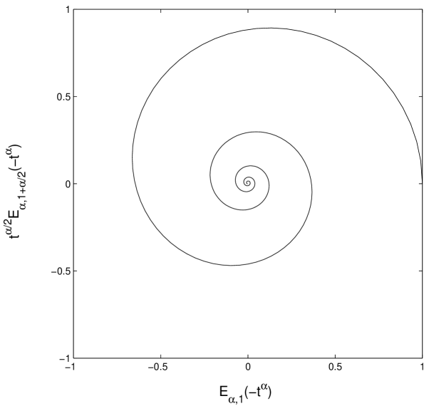
Figure 1: Phase plane diagram of the fractional oscillator with the initial conditions $q_{\alpha}(0)=1$, $\tilde{D}^{\alpha}q_{\alpha}(0)=0$, where $\alpha=1.8$.

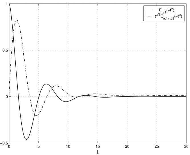
Figure 2: Fractional oscillations are characterized by a finite number of zeros ($\alpha=1.65$).

As is shown in 14ac ; 16 , the fractional oscillations exhibit a finite number of damped oscillations with an algebraic decay (Fig. 2). The fact rests on that such oscillations may be decomposed into two parts. One of them demonstrates asymptotically an algebraic (monotonic) decay, and another term represents an exponentially damped harmonic oscillation. Owing to the second term decreasing faster than this happens for the term with an algebraic decay, the fractional oscillations possess a finite number of zeros. Our notation $\omega_{0}$ named as a circular frequency is enough acceptable, since the value characterizes the number of oscillations on a given temporal interval.

5 Effect of fractional damping on resonance

Now we consider a behavior of the fractional oscillator under an external force. Following the initial conditions $x(0)=0$ and $\dot{x}(0)=0$, this model is described by the following equation

$$x(t) = -\frac{\omega^{\alpha}_{0}}{\Gamma(\alpha)}\int^{t}_{0}(t-t^{\prime})^{\alpha-1}\,x(t^{\prime})\,dt^{\prime}+$$ (9)

$$+ \frac{1}{\Gamma(\alpha)}\int^{t}_{0}(t-t^{\prime})^{\alpha-1}\,F(t^{\prime})\,dt^{\prime}\,,$$

where it should be kept $1<\alpha<2$, and $F$ is the external force. The dynamic response of the driven fractional oscillator was investigated in 15 :

$$x(t)=\int^{t}_{0}F(t^{\prime})\,(t-t^{\prime})^{\alpha-1}\,E_{\alpha,\,\alpha}(-\omega^{\alpha}_{0}(t-t^{\prime})^{\alpha})\,dt^{\prime}\,.$$ (10)

This allows us to define the response for any desired forcing function $F(t)$. The “free” and “forced” oscillations of such a fractional oscillator depend on the index $\alpha$. However, in the first case the damping is characterized only by the “natural frequency” $\omega_{0}$, whereas the damping in the case of “forced” oscillations depends also on the driving frequency $\omega$. Each of these cases has a characteristic algebraic tail associated with damping 16a .

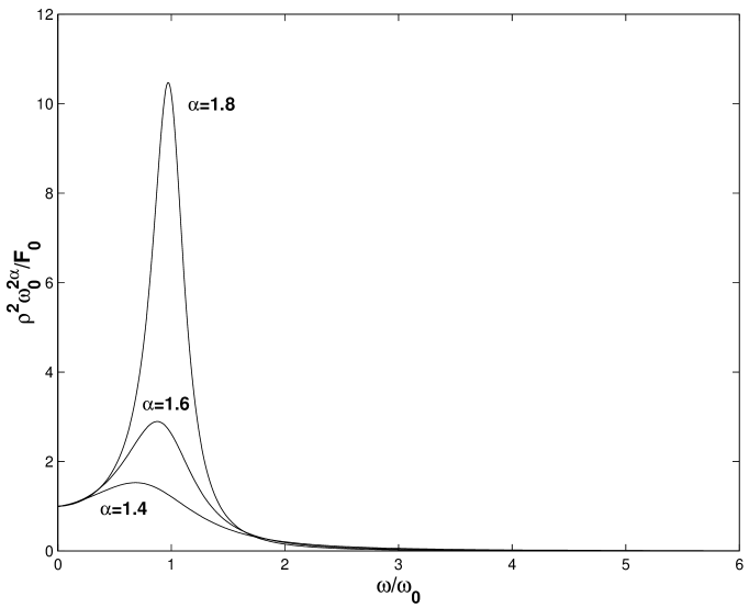
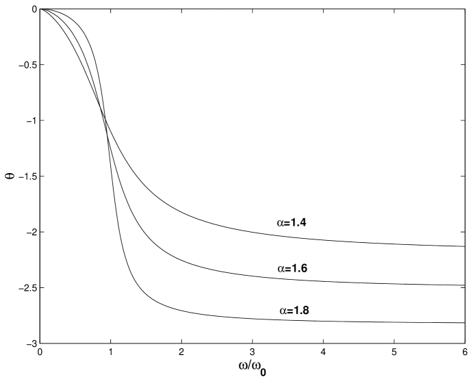
Figure 3: Resonance curves and phase shift of the fractional oscillator forced by an harmonic oscillation with the frequency $\omega$.

If $F(t)$ is periodic, namely $F(t)=F_{0}\,e^{j\omega t}$, then the solution of Eq. (9) is determined by taking the inverse Laplace transform

$$x(t)=\frac{1}{2\pi j}\int_{Br}e^{st}\frac{F_{0}\,(s+j\omega)\,ds}{(s^{2}+\omega^{2})\,(s^{\alpha}+\omega_{0}^{\alpha})}\,.$$ (11)

The Bromwich integral (11) can be evaluated in terms of the theory of complex variables. Some particular examples of driving functions in this context were considered in 15 . However, the case under interest was studied in 15a . Consider only the harmonically forced oscillation. If one waits for a long enough time, the normal mode in this system is damped. After the substitution $x_{0}e^{j\omega t}$ for $x(t)$ in Eq.(9) we obtain

$$x_{0}\,e^{j\omega t} = -\frac{\omega^{\alpha}_{0}}{\Gamma(\alpha)}\int^{t}_{0}(t-t^{\prime})^{\alpha-1}\,x_{0}\,e^{j\omega t^{\prime}}\,dt^{\prime}+$$ (12)

$$+ \frac{1}{\Gamma(\alpha)}\int^{t}_{0}(t-t^{\prime})^{\alpha-1}\,F_{0}\,e^{j\omega t^{\prime}}\,dt^{\prime}\,.$$

It is convenient to change the variable $\omega(t-t^{\prime})=\zeta$ in the integrand. Next we can divide out $\exp(j\omega t)$ from each side of (12) and direct $t$ to infinity. The procedure permits one to extract the contribution of steady-state oscillations. Then Eq. (12) gives

$$x_{0}=\frac{F_{0}}{[\omega_{0}^{\alpha}+\omega^{\alpha}\exp(j\pi\alpha/2)]}\,.$$ (13)

The forced solution $\rho\exp(j\omega t+\theta)$ is written as

$$\rho^{2} =\frac{F_{0}}{[\omega_{0}^{2\alpha}+\omega^{2\alpha}+2\omega_{0}^{\alpha}\omega^{\alpha}\cos(\pi\alpha/2)]}\,,$$

$$\tan\theta =-\frac{\omega^{\alpha}\sin(\pi\alpha/2)}{\omega_{0}^{\alpha}+\omega^{\alpha}\cos(\pi\alpha/2)}\,.$$

Denote $\omega/\omega_{0}=z$. Then we have

$$\frac{\rho^{2}\omega_{0}^{2\alpha}}{F_{0}} = \frac{1}{[z^{2\alpha}+2z^{\alpha}\cos(\pi\alpha/2)+1]}\,,$$

$$\tan\theta = -\frac{z^{\alpha}\sin(\pi\alpha/2)}{1+z^{\alpha}\cos(\pi\alpha/2)}\,.$$ (14)

It should be noticed that the maximum of $\rho^{2}\omega_{0}^{2\alpha}/F_{0}$ is not attained for $\omega=\omega_{0}$. It is shifted to the origin of coordinates on Fig. 3 with decaying $\alpha$. To differentiate $\rho^{2}\omega_{0}^{2\alpha}/F_{0}$ with respect to $z$, we get the maximum $z_{max}=\sqrt[\alpha]{\cos[\pi(2-\alpha)/2]}$. For $\alpha=2$ the damping in this oscillator vanishes. If then both frequencies coincide $\omega=\omega_{0}$, the amplitude of the oscillator tends to infinity.

6 Coupled fractional oscillators

From the theory of vibrations it is well known, much of physical systems permits a description in the form of free harmonic oscillators. However, such a representation is too idealized, as in many practical cases these systems are not usually isolated. Instead, they interact with environment, or with other oscillators. Therefore, the study of the dynamics of driven and coupled oscillators is of major importance.

Here we intend to provide a similar analysis for fractional systems. Consider two identical fractional oscillators mutually coupled. For $1<\alpha\leq 2$ the dynamics of this system is given by

$$\tilde{D}^{\alpha}x_{1}+\omega_{0}^{2}x_{1}+\kappa^{2}(x_{1}-x_{2}) = 0\,,$$ (15)

$$\tilde{D}^{\alpha}x_{2}+\omega_{0}^{2}x_{2}+\kappa^{2}(x_{2}-x_{1}) = 0\,,$$ (16)

where the two oscillators are labelled by 1 and 2, respectively, and $\kappa^{2}$ is the measure of the coupling, $\omega_{0}$ the circular frequency. Let us introduce new variables $u_{1}=x_{1}+x_{2}$ and $u_{2}=x_{1}-x_{2}$. In such coordinates the system of equations (15), (16) transforms into the equations of two independent fractional oscillators with the frequencies $\omega_{0}$ and $\sqrt{\omega_{0}^{2}+2\kappa^{2}}$. If $u_{2}=0$, then $x_{1}=x_{2}$ so that both oscillators move in phase with the frequency $\omega_{0}$. In this case the coupling between the oscillators has no influence on their motion. If $u_{1}=0$ or $x_{1}=-x_{2}$ that is the same, the oscillators evolve in antiphase with the increased frequency $\sqrt{\omega_{0}^{2}+2\kappa^{2}}$ in force of the measure of the coupling.

It is often found that the physical systems of interest consist of two and more oscillators which interact weekly among them. When the coupling is weak ($\kappa\ll 1$), the fractional oscillators transfer their energy from ones to others and vice versa. The effect depends on the magnitude of the index $\alpha$ characterizing a strength of dissipation as well as on the magnitude of the parameter $\kappa$. Nevertheless, due to the dissipation, finally the fractional oscillations will decrease in amplitude.

Let two oscillators rest initially. Then one of them gets $\tilde{D}^{\alpha/2}x_{1}(0)=B_{0}$. Following Sect. 4, the time evolution of this system takes the form

$$x_{1}(t)=\frac{B_{0}}{2}\Bigl{[}\omega_{0}t^{\alpha/2}E_{\alpha,\,1+\alpha/2}(-\omega^{2}_{0}t^{\alpha})+$$

$$+\,t^{\alpha/2}E_{\alpha,\,1+\alpha/2}(-(\omega_{0}^{2}+2\kappa^{2})t^{\alpha})\Bigr{]}\,,$$ (17)

$$x_{2}(t)=\frac{B_{0}}{2}\Bigl{[}\omega_{0}t^{\alpha/2}E_{\alpha,\,1+\alpha/2}(-\omega^{2}_{0}t^{\alpha})-$$

$$-\,t^{\alpha/2}E_{\alpha,\,1+\alpha/2}(-(\omega_{0}^{2}+2\kappa^{2})t^{\alpha})\Bigr{]}\,.$$ (18)

Fig. 4 shows a superposition of two fractional oscillations. The oscillations observable are complicated, but they can be likened to damping beats. In the force of this damping the minimum of $x_{1}$ does not coincide with the maximum of $x_{2}$. The phase shift between them is determined by the value $\alpha$, i. e. by the level of dissipation in this system. Moreover, the algebraic relaxation term of the fractional oscillations deforms the position of the maxima of $x_{1}$ and $x_{2}$. Distinctly this can be seen in Fig. 4b .

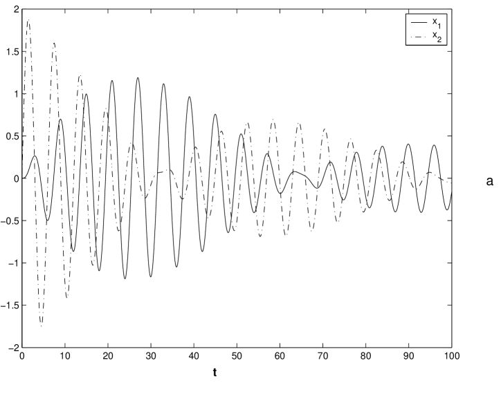
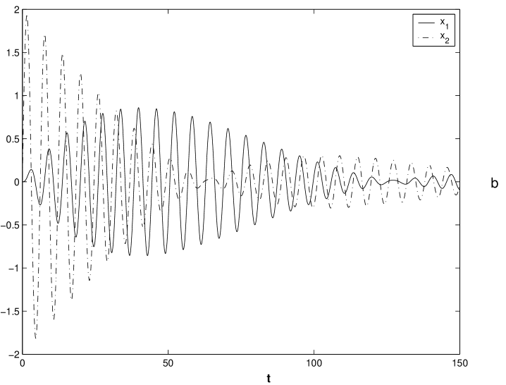
Figure 4: Superposition of two modes ($x_{1}$ and $x_{2}$) with $\alpha=1.98,\omega_{0}=1$: a) $\kappa=0.3162$; b) $\kappa=0.2236$.

The decomposition of the dynamics of coupled fractional oscillators in a superposition of normal modes,    which are simple fractional oscillators, is a major result in the physics of coupled fractional oscillators. This decomposition is not restricted to just two coupled oscillators. An analogous decomposition holds for an arbitrary large number of coupled fractional oscillators.

7 Forced oscillations of a multiple fractional system

Let a fractional oscillator have two degree of freedom. The harmonic force with the frequency $p$ acts on the system coordinates $x$ and $y$. Then the equations of motion are written as

$$\cases{A\tilde{D}^{\alpha}x+H\tilde{D}^{\alpha}y+ax+hy=X\cos pt\,,\cr H\tilde{D}^{\alpha}x+B\tilde{D}^{\alpha}y+hx+by=Y\cos pt\cr}$$ (19)

with $1<\alpha\leq 2$. We shall seek solutions to Eqs. (19) in the form

$$x=\beta\cos pt\,,\qquad\qquad y=\gamma\cos pt\,.$$

The treatment of dynamical equations can be greatly simplified by using the representation in complex numbers. With this object in view, replace $\cos pt$ by $e^{jpt}$ in (19). Next we substitute $x=\beta e^{jpt}$ and $y=\gamma e^{jpt}$ in such a system of equations. Pick out $e^{jpt}$ in each term of the equations. The fractional derivative of $e^{jpt}$ gives

$$\tilde{D}^{\alpha}e^{jpt} = J^{2-\alpha}D^{2}e^{jpt}=-p^{2}J^{2-\alpha}e^{jpt}=$$

$$= -\frac{p^{\alpha}e^{jpt}}{\Gamma(m)}\int_{0}^{pt}\tau^{m-1}\,e^{-j\tau}\,d\tau\,,$$

where $m=2-\alpha$ is constant. Making $t\to\infty$ in the above integral, we apply the table integral 17 :

$$\int_{0}^{\infty}z^{\xi-1}\,e^{-jz}\,dz=\Gamma(\xi)\,e^{-j\pi\xi/2}$$

for $0<{\rm Re}\,\xi<1$. This technique transforms Eqs. (19) into the algebraic expressions

$$\cases{(a+A\,p^{\alpha}e^{j\pi\alpha/2})\beta+(h+H\,p^{\alpha}e^{j\pi\alpha/2})\gamma=X\,,\cr(h+H\,p^{\alpha}e^{j\pi\alpha/2})\beta+(b+B\,p^{\alpha}e^{j\pi\alpha/2})\gamma=Y\,.\cr}$$ (20)

The steady-state solutions of Eqs. (19) can be derived from (20) by taking the “real” part of $\beta$ and $\gamma$, i. e. by projecting the motion onto the real axis of $x$ and $y$. From Eqs.(20) at once it follows that

$$\beta=\frac{1}{\Delta}\left|\begin{array}[]{lllll}X&h+H\,p^{\alpha}e^{j\pi\alpha/2}\\ Y&b+B\,p^{\alpha}e^{j\pi\alpha/2}\\ \end{array}\right|\,,$$ (23)

$$\gamma=\frac{1}{\Delta}\left|\begin{array}[]{lllll}a+A\,p^{\alpha}e^{j\pi\alpha/2}&X\\ h+H\,p^{\alpha}e^{j\pi\alpha/2}&Y\\ \end{array}\right|\,,$$ (26)

where

$$\Delta=\left|\begin{array}[]{lllll}a+A\,p^{\alpha}e^{j\pi\alpha/2}&h+H\,p^{\alpha}e^{j\pi\alpha/2}\\ h+H\,p^{\alpha}e^{j\pi\alpha/2}&b+B\,p^{\alpha}e^{j\pi\alpha/2}\\ \end{array}\right|$$

is the determinant. Thus the general conclusion is the following. When a periodic force of simple-harmonic type acts on any part of the system, every part executes a simple-harmonic vibration of the same period, but the amplitude will be different in different parts. When the period of the forced vibration nearly coincides with one of the free modes, an abnormal amplitude of forced vibration will be in general result, owing to the smallness of the denominator on the formulae (26).

If $X\neq 0$, $Y=0$, then

$$\gamma=-\frac{X(h+H\,p^{\alpha}e^{j\pi\alpha/2})}{\Delta}\,.$$ (27)

Imagine now a second case of forced vibration in which $X=0$, $Y\neq 0$. This yields

$$\beta=-\frac{Y(h+H\,p^{\alpha}e^{j\pi\alpha/2})}{\Delta}\,.$$

Comparing with (27), we see that

$$\gamma:X=\beta:Y\,.$$ (28)

The result concerns a remarkable theorem of reciprocity, first proved for the theory of aerials by Helmholtz, and afterwards greatly extended by Rayleigh. Their interpretation is most easily expressed when the “forces” $X$, $Y$ are of the same character in such a way that we may put $X=Y$ and obtain $\beta=\gamma$. The coupled fractional oscillators forced by harmonic oscillations support well the theorem. Indeed, it is clear in view of their equations of motion being linear.

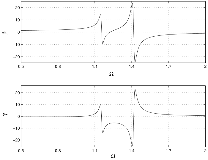
Figure 5: Resonance curves of the fractional oscillator forced with two degree of freedom: $X=3$, $Y=0$, $\alpha=1.99,H=h=1,A=B=2,a=b=3$. The dynamical damping is detectable, when $\beta=0$ and $\gamma\neq 0$. See text for more details.

The resonance curves are represented in Fig. 5. Here we consider the case, when $X\neq 0$, $Y=0$. The curves demostrate the following interesting effects: 1) if the exterior force frequency $\Omega$ coincides with one of normal frequencies of this system, the amplitudes of both oscillators increase; 2) if the frequency of the exterior force, acting on the first oscillator, coincides with $\sqrt[\alpha]{b/\{B\cos(\pi(2-\alpha)/2)\}}>0$, then the first oscillator is rest ($\beta=0$). The latter phenomenon is called the dynamic damping often used for the breaking of unfavourable oscillations 18 . For the exterior force frequency $\sqrt[\alpha]{h/\{H\cos(\pi(2-\alpha)/2)\}}>0$ the second oscillator will be rest.

The extension of the method to the general case of linear fractional oscillations of a multiple system is obvious so that the result may be stated formally. In such a system with $k$ degrees of freedom there are in general $k$ distinct “normal modes” of free fractional vibrations about a configuration of stable equilibrium, the frequencies of which are given by a symmetrical determinantal equation of the $k$-th order in $p^{\alpha}e^{j\pi\alpha/2}$, analogous to (20). In each of these modes the system oscillates exactly as if it had only one degree of freedom.

8 Transition to continuous systems

At least mathematically, it is sometimes possible to pass from the study of oscillatory systems of finite freedom to continuous systems by a sort of limiting process. So D. Bernoulli (1732) considered the vibrations of a hanging chain as a limiting form of the problem where a large number of equal and equidistant particles are attached to a tense string whose own mass is neglected. The general principles may be applied to fractional systems too. In this section we shall be concerned with fractional systems for which the number of degrees of freedom becomes infinite.

The lattice represents the most illustrative example which is naturally called by the ordered structure of oscillators. To start with an one-dimensional chain of identical fractional oscillators, the characteristic spatial period of wave motion in this chain is assumed to be too more than the mesh dimension. If the oscillators interact with the nearest neighbours, they are described by the equations of type

$$\frac{d^{\alpha}\phi_{n}}{dt^{\alpha}}+\omega_{0}^{2}\phi_{n}=M(\phi_{n-1}+\phi_{n+1}-2\phi_{n})\,,$$ (29)

where $M$ is constant, and $1<\alpha\leq 2$. Proceeding from the discrete system to a continuous one, we arrive at the equation in partial derivatives

$$\frac{\partial^{\alpha}\phi}{\partial t^{\alpha}}-v^{2}\,\frac{\partial^{2}\phi}{\partial x^{2}}+\omega^{2}_{0}\phi=0\,,$$ (30)

where $v^{2}=Ma^{2}$, and $a$ is the mesh size. If $\omega_{0}=0$, the equation (30) is simplified so that its solution is

$$\phi(x,t)=\int_{0}^{\infty}p^{S}(t,\tau)\,\Bigl{\{}f_{1}(v\tau-x)+f_{2}(v\tau-x)\Bigr{\}}\,d\tau,$$ (31)

where the functions $f_{1}$, $f_{2}$ are arbitrary. The two terms in (31) admit of a simple interpretation. They represent damped-in-time waveforms traveling in the direction of $x$-positive and $x$-negative.

In this connection it should be necessarily mentioned that for $0<\alpha\leq 1$   Eq. (30) will describe an anomalous diffusion with a potential. Then the function $\phi(x,t)$ becomes a probability density. Thus the value has quite an other interpretation 19 in comparison with the above-mentioned case.

9 Interpretation and discussion

Nature is permeated with oscillatory phenomena. Pulsating stars and earthquakes, oscillating chemical reactions and long term variations of the Earth’s magnetic fields, circadian rhythms and beats of the heart, electromagnetic waves and modes of oscillation of the atom nucleus are examples of this kind of phenomena among many others. Electrical and mechanical oscillators are everyday constituents in the world of engineering. Usually an oscillator is something that behaves cyclically, changing in some way, but eventually getting back to where it started again. The fractional calculus extends our representation about oscillatory phenomena. The temporal evolution of fractional oscillator models occupies an intermediate place between exponential relaxation and pure harmonic oscillations. The fractional oscillator clearly demonstrates a pure algebraic decay together with an exponentially damped harmonic motion.

The modification of the conventional representation of the Hamilton equations is conditioned on a random interaction of the subsystems with environment. Each subsystem is governed by its own internal clock. Although its dynamics is described by the ordinary Hamiltonian equations,    their coordinates and momenta depend on the operational time. The passage from the operational time to the physical time through the averaging procedure accounts for the interaction of the subsystem with environment. Consequently, the whole of subsystems behaves as a fractional system.

The author thanks D. Dreisigmeyer for fruitful discussions.

References

- (1) G. M. Zaslavsky, Phys. Rep. 371, 461 (2002)
- (2) R. Metzler, J. Klafter, Phys. Rep. 339, 1 (2000)
- (3) K. Weron, A. Klauser, Ferroelectrics 236, 59 (2000)
- (4) G. M. Zaslavsky,Hamiltonian Chaos and Fractional Dynamics (Oxford University Press, 2005)
- (5) F. Mainardi, “Fractional calculus: some basic problems in continuum and statistical mechnics”, In: A. Carpinteri and F. Mainardi (eds.), Fractals and Fractional Calculus in Continuum Mechanics (Springer-Verlag, New York, 1997), pp. 291-348
- (6) J. Bisquert, Phys. Rev. Lett. 91, 010602 (2003)
- (7) A. V. Chechkin, V. Y. Gonchar, M. Szydłowsky, Phys. Plasma 9, 78 (2002)
- (8) A. A. Stanislavsky, JETP 98, 705 (2004)
- (9) S. Boldyrev, C. R. Gwinn, Phys. Rev. Lett. 91, 131101 (2003)
- (10) M. Seredyńska, A. Hanyga, J. Math. Phys. 41, 2135 (2000)
- (11) A. M. Lacasta, J. M. Sancho, A. H. Romero, I. M. Sokolov, K. Lindenberg, Phys. Rev. E 70, 051104 (2004)
- (12) V. E. Tarasov, G. M. Zaslavsky, Physica A 354, 249 (2005)
- (13) F. Riewe, Phys. Rev. E 53, 1890 (1996); F. Riewe, Phys. Rev. E 55, 3581 (1997)
- (14) O. P. Agrawal, J. Math. Anal. Appl. 272, 368 (2002)
- (15) S. Muslih, D. Baleanu, Czech. J. Phys 5, 633 (2005)
- (16) D. W. Dreisigmeyer, P. M. Young, J. of Phys. A: Math. Gen. 36, 8297 (2003)
- (17) D. W. Dreisigmeyer, P. M. Young, J. of Phys. A: Math. Gen. 37, L117 (2004)
- (18) V. E. Tarasov, Chaos 14, 123 (2004); V. E. Tarasov, J. of Physics: Conference Series (IOP) 7, 17 (2005)
- (19) V. M. Zolotarev, One-dimensional Stable Distributions (American Mathematical Society, Providance, 1986)
- (20) N. H. Bingham, Z. Wharsch. verw. Geb. 17, 1 (1971)
- (21) A. A. Stanislavsky, Phys. Rev. E 67, 021111 (2003)
- (22) M. M. Meerschaert, H.-P. Scheffler, J. Appl. Probab. 41, 623 (2004)
- (23) F. Mainardi, Chaos, Solitons & Fractals 7, 1461 (1996)
- (24) C. Fox, Trans. Amer. Math. Soc. 98, 395 (1961)
- (25) W. Feller, An Introduction to Probability Theory and Its Aplications (Wiley, New York, 1971)
- (26) I. M. Sokolov, Phys.Rev. E 63, 056111 (2001)
- (27) I. M. Sokolov, J. Klafter, Chaos 15, 026103 (2005)
- (28) A. I. Saichev, G. M. Zaslavsky, Chaos 7, 753 (1997)
- (29) R. Metzler, Phys. Rev. E 62, 6233 (2000)
- (30) A. A. Stanislavsky, Physica A 318, 469 (2003)
- (31) I. Goychuk, P. Hnggi, Phys. Rev. E 70, 051915 (2004)
- (32) A.A. Stanislavsky, Phys. Scripta 67, 265 (2003)
- (33) R. Metzler, J. Klafter, J. Phys. A: Math. Gen. 37, R161 (2004)
- (34) A. Piryatinska, A. I. Saichev, W. A. Woyczynski, Physica A 349, 375 (2005)
- (35) Yu. Rabotnov, Creep problems in structural members (North-Holland, Amsterdam, 1969), p. 129. Originally published in Russian as: Polzuchest’ Elementov Konstruktsii (Nauka, Moscow, 1966)
- (36) M. Caputo, Geophys. J. Roy. Astron. Soc. 13, 529 (1967)
- (37) R. Gorenflo, F. Mainardi, “Fractional calculus: integral and differential equations of fractional order”, In: A. Carpinteri and F. Mainardi (eds.) Fractals and Fractional Calculus in Continuum Mechanics (Springer-Verlag, New York, 1997), pp. 223-276
- (38) K. B. Oldham, J. Spanier, The Fractional Calculus (Academic Press, New York, 1974)
- (39) I. Podlubny, Fractional Differential Equations (Academic Press, San Diego, 1999)
- (40) B. N. Narahari Achar, J. W. Hanneken, T. Enck, T. Clarke, Physica A 287, 361 (2001)
- (41) A. A. Stanislavsky, Phys. Rev. E 70, 051103 (2004)
- (42) A. A. Stanislavsky, Physica A 354, 101 (2005)
- (43) B. N. Narahari Achar, J. W. Hanneken, T. Clarke, Physica A 309, 275 (2002)
- (44) M. Abramowitz, I. Stegun, Handbook of Mathematical Functions (Dover, New York, 1972)
- (45) A. A. Andronov, A. A. Vitt, S. E. Khaikin, Theory of Oscillators (Pergamon, Oxford, 1966)
- (46) A. A. Stanislavsky, Theor. and Math. Phys. 138, 418 (2004)