Renormalization group analysis of the $M$-$p$-spin glass model with $p=3$ and $M=3$

Abstract

We study an $M$-$p$-spin spin glass model with $p=3$ and $M=3$ in three dimensions using the Migdal-Kadanoff renormalization group approximation (MKA). In this version of the $p$-spin model, there are three ($M=3$) Ising spins on each site. At mean-field level, this model is known to have two transitions; a dynamical transition and a thermodynamic one at a lower temperature. The dynamical transition is similar to the mode-coupling transition in glasses, while the thermodynamic transition possibly describes what happens at the Kauzmann temperature. We find that all the coupling constants in the model flow under the MKA to the high-temperature sink implying that the mean-field features disappear in three dimensions and that there is no transition in this model. The behavior of the coupling constant flow is qualitatively similar to that of the model with $p=3$ and $M=2$, for which only a single transition is predicted at the mean-field level. We conclude that for $p$-spin models in three dimensions, fluctuation effects completely remove all traces of their mean-field behavior.

Understanding the dynamics and thermodynamics of supercooled liquids and structural glasses is one of the most challenging problems in condensed matter physics. Theoretical advances have been made using an idea obtained from certain mean-field spin glass models KTW . One example is the infinite-range $p$-spin spin glass model KTW , which shows two phase transitions. There is a dynamical transition at a temperature $T_{d}$ below which an ergodicity breaking occurs. The connection to structural glasses comes from the similarity of the dynamical equations of these spin glass models near $T_{d}$ to those in the mode-coupling theory of the structural glass transition MCT . Below the dynamical transition, a thermodynamic transition takes place at $T_{0}$ with the low temperature phase described by the one-step replica symmetry breaking (RSB). This transition has been associated with a possible transition at the Kauzmann temperature $T_{K}$ Kauzmann in structural glasses. An important question is then how this mean-field picture gets changed in finite dimensions. Beyond the mean-field level, the dynamical transition at $T_{d}$ is expected to disappear because of activation processes over finite energy barriers separating metastable states. However, the thermodynamic glass transition $T_{0}$ could still exist in principle in finite dimensional systems. In this paper, we use the Migdal-Kadanoff (MK) real space renormalization group (RG) method to investigate this issue.

The original $p$-spin glass model mentioned above, however, is inconvenient to study on a simple hypercubic lattice. In Ref. PPR , a new class of $p$-spin glass models called the $M$-$p$-spin glass model has been proposed. These models consist of Ising spins on a hypercubic lattice with nearest-neighbor $p$-body interactions. The new feature of these models is that there are $M$ Ising spins on each site. As the value of the parameters $M$ and $p$ change, these models exhibit two distinct types of behavior at mean-field (MF) level. For example, when $p=3$ and $M=2$, the model at mean-field level has a single continuous transition to a full RSB state. On the other hand, for $p=3$ and $M=3$, one has the two transitions described above. One can actually classify all these models for general $p$ and $M$, into the two mean-field transition types mpspin . Therefore the $M$-$p$-spin glass model is an ideal testbed for studying how thermal fluctuations change mean-field results. The $p=3$, $M=2$ model has been studied by Monte Carlo simulations in four dimensions PPR and the results were interpreted as evidence for a single continuous transition. The Migdal-Kadanoff RG has been applied DBM ; MD to this model, using versions to mimic both three and four dimensions, and it was shown that the coupling constants flow to the high-temperature sink implying that there is no transition in both these dimensions. This model has been shown MD to be in the same universality class as the Ising spin glass in a field, which is consistent with the absence of a phase transition in less than six dimensions AT . The correlation length obtained from the Migdal-Kadanoff RG grows quite rapidly with decreasing temperature to a value of order $30$ lattice spacings. Thus in a numerical simulation of a finite system whose linear extent is of order $10$ lattice spacings, it is therefore very likely that the rapidly growing correlation length seen would appear to be implying there is a transition PPR , but this would just be an artifact of finite size effects. The non-mean-field regime of the $p=3$ and $M=2$ model has also been simulated using a one-dimensional long-ranged Ising spin glass where the couplings decrease with their separation $r_{ij}$ as $\sim 1/r_{ij}^{\sigma}$. By varying the exponent $\sigma$ one can effectively tune the one-dimensional system to have similarities to the short-range problem in spatial dimension $d$ Larson . The mean-field transition was shown to be destroyed at values of $\sigma$ which correspond to low values of $d$.

It is a purpose of this paper to find whether the mean-field transitions in the $p=3$ and $M=3$ model, which are relevant to discussions on structural glasses, survive to three dimensions using the Migdal-Kadanoff real space RG. The MKA is an approximate RG procedure which works best in low-dimensions $d$ such as two and three where it gives excellent results for the Ising (i.e. $p=2$) spin glass.

The $M$-$p$-spin model we study in this paper is characterized by $M$ Ising spins $\sigma^{(\alpha)}_{i}$, $\alpha=1,2,\cdots,M$ on each site $i$ of a hypercubic lattice. The Hamiltonian is given in terms of products of $p$ spins chosen from the spins in a pair of nearest neighbor sites. In this paper, we focus on the $p=3$ case and the Hamiltonian of the 3-spin glass model is given by

$$\mathcal{H} = -\sum_{\langle ij\rangle}\sum^{M}_{\alpha<\beta}\sum^{M}_{\gamma}\Big{(}J^{(\alpha\beta)\gamma}_{ij}\sigma^{(\alpha)}_{i}\sigma^{(\beta)}_{i}\sigma^{(\gamma)}_{j}$$ (1)

$$\quad\quad\quad\quad\quad\quad+J^{\gamma(\alpha\beta)}_{ij}\sigma^{(\gamma)}_{i}\sigma^{(\alpha)}_{j}\sigma^{(\beta)}_{j}\Big{)},$$

where the notation $\langle ij\rangle$ means that the sum is over all nearest neighbor pairs $i$ and $j$. Note that the number of different coupling constants, $J^{(\alpha\beta)\gamma}_{ij}$ and $J^{\gamma(\alpha\beta)}_{ij}$ for given $\langle ij\rangle$ is just $2M\binom{M}{2}=M^{2}(M-1)$. All these couplings are chosen independently from a Gaussian distribution with zero mean and width $J$. Therefore for the 3-spin glass models, there are 4 and 18 independent couplings for $M=2$ and $M=3$, respectively.

The above $M$-$p$-spin model can be put into a field theoretical framework. A standard way to do this is to use the Hubbard-Stranotovich transformation on the replicated partition function and then trace over the spins. The resulting field theory associated with this model is the following Ginzburg-Landau-Wilson Hamiltonian

$$\mathcal{H}_{\mathrm{GLW}} = \int d^{d}\mathbf{r}\Bigg{\{}\frac{1}{2}\sum_{a<b}[\nabla q_{ab}(\mathbf{r})]^{2}+\frac{t}{2}\sum_{a<b}q^{2}_{ab}(\mathbf{r})$$ (2)

$$\quad\quad-\frac{w_{1}}{6}\mathrm{Tr}q^{3}(\mathbf{r})-\frac{w_{2}}{3}\sum_{a<b}q^{3}_{ab}(\mathbf{r})\Bigg{\}},$$

where $q_{ab}(\mathbf{r})$ is the order parameter and $a$ and $b$ are replica indices running from 1 to $n$ with $n\to 0$. At mean field level, this model is known Gross to show very different behavior depending on the value of $R=w_{2}/w_{1}$. When $R>1$, there are two transitions at the mean field level as described above; a dynamical transition at some temperature $T_{d}$ and a thermodynamic transition at a lower temperature $T_{0}$ to a state with one-step replica symmetry breaking. The two transitions have been discussed extensively in connection with what happens in structural glasses near the mode-coupling and the Kauzmann temperatures, respectively. For the case where $R<1$, only a single transition to a state with full RSB is expected at mean-field level. In Ref. mpspin , the ratio $R$ was evaluated for the $M$-$p$-spin model for general values of $M$ and $p$. The cases we are interested in this paper, namely $p=3,M=2$ and $p=3,M=3$, correspond to $R=3(1-1/\sqrt{2})\simeq 0.879$ and $R=2$, respectively. Therefore the two models show very different mean-field behavior. It is the purpose of this paper to investigate how thermal fluctuations affect the two kinds of mean-field behavior in three dimensions.

To do this we apply the Migdal-Kadanoff real space RG to these models. We follow closely the approximate bond moving scheme described in detail in Ref. DBM . For a three dimensional cubic lattice, four bonds are put together to form a new bond. The coupling constant of this new bond is just given by the sum of the coupling constants of the four bonds. We can obtain a coarse grained lattice by taking a trace over the spins at the site connecting two new bonds. The decimation procedure can be continued $n$ times for a system of size $L=2^{n}$. Although we initially start from only the three-spin couplings $K^{(\alpha\beta)\gamma}\equiv J^{(\alpha\beta)\gamma}/T$ and $K^{\gamma(\alpha\beta)}\equiv J^{\gamma(\alpha\beta)}/T$ drawn from a Gaussian distribution with standard deviation (width) $K\equiv J/T$ at temperature $T$, the decimation procedure generates additional types of couplings as well as on-site “field” terms which involve the spins only on one site. In the Migdal-Kadanoff analysis, we have to keep track of all these couplings.

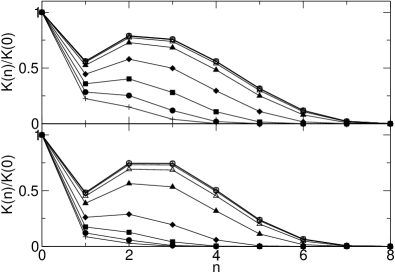
Figure 1: RG flow of the three-spin coupling strength $K(n)/K(0)$ normalized with its initial value at iteration step $n$. The upper panel is for $p=3$ and $M=3$, and the lower one for $p=3$, $M=2$. One each panel, the curves correspond from bottom to top to temperatures $T/J=10,8,6,4,2,1,0.5,0.25$ and 0.1.

For the $p=3$, $M=2$ case, on each bond there are initially four three-spin couplings. In addition to those, we have to consider four two-spin couplings and one coupling that involves all the four spins on the nearest-neighbor sites. There are also four field terms on the two nearest neighbor sites and two on-site terms involving two spins on one site. If we include a constant contribution to the Hamiltonian, the renormalized Hamiltonian carries a total of 16 coupling constants. For the $p=3$, $M=3$ case, on the other hand, each bond is connected to 6 spins, 3 spins on each site. There are couplings involving 2, 3, 4, 5 and 6 spins from a pair of nearest neighbor sites, whose standard deviations are denoted by $C$, $K$, $D$, $E$ and $F$, respectively. The numbers of independent coupling constants connecting 2, 3, 4, 5 and 6 spins are given by 9, 18, 15, 6 and 1, respectively. There are also on-site terms. The numbers of on-site fields involving 1, 2 and 3 spins are 6, 6 and 2, respectively. Including a constant term, we have to keep track of a total 64 couplings in the case of $p=3$ and $M=3$.

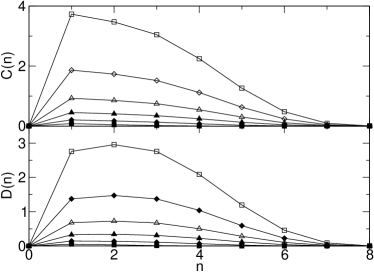
Figure 2: RG flow of the two-spin coupling $C(n)$ and the four-spin coupling $D(n)$ of the $p=3$, $M=3$ model at the $n$-th iteration step. The curves correspond from bottom to top to temperatures $T/J=8,4,2,1,0.5$ and 0.25.

A key step in the calculation is setting up and solving the recursion relation resulting from the decimation procedure. For $p=3$ and $M=3$, this amounts to solving a system of 64 simultaneous equations for a new set of couplings, which requires an inversion of a constant $64\times 64$ matrix. This only needs to be done once beforehand and not for every iteration. In the actual numerical calculations, $10^{6}$ bonds are prepared. On each bond 18 three-spin couplings, $K^{(\alpha\beta)\gamma}$ and $K^{\gamma(\alpha\beta)}$ are chosen independently from the Gaussian distribution with zero mean and width $K(0)=J/T$ at temperature $T$. All the other couplings including the fields are set to zero initially. We then randomly choose two sets of 4 bonds to form two new bonds. Using the recursion relation, we obtain a set of 64 renormalized couplings. This procedure is continued until we get $10^{6}$ new bonds, which completes the first iteration. As we iterate the same procedure, we can obtain the flow of 64 couplings. At each step of the iteration, we evaluate the width of each distribution. We note that there is a certain freedom in where to move on-site fields when the four bonds are put together. The main results do not depend on the method chosen. We follow the prescription given in Ref. DBM : when three bonds are moved to combine with a bond, the fields on the three bonds are placed at the site that is to be traced over.

The RG flow of the width of the three-spin coupling $K(n)$ at the $n$-th iteration normalized with the initial value $K(0)=J/T$ is shown in Fig. 1 for the 3-spin glass model with $M=3$ and $M=2$, respectively. Somewhat surprisingly, both figures show essentially the same features. At all temperatures, the couplings decrease to zero in the long length scale limit indicating an RG flow to the high temperature sink. This implies that there is no finite temperature phase transition in these models in contrast to the corresponding mean-field pictures. At high temperatures, the coupling simply decreases to zero. As the temperature is reduced, however, the coupling increases during the first few iterations reaching a maximum at the second or third iteration, but eventually decaying to zero. At very low temperatures $T/J\lesssim 0.25$, the flow patterns of $K(n)/K(0)$ reach an asymptotic form. The only difference between $M=3$ and $M=2$ cases is that the couplings in the $M=3$ model decay to zero more slowly as the iteration proceeds. We can deduce from this that the correlation length in the $M=3$ model is longer than that of the $M=2$ model.

The other couplings for the $p=3$ and $M=3$ model also flow to zero as can be seen from Fig. 2. The upper panel shows the RG flow of the width $C(n)$ of the two-spin couplings for various temperatures, which reaches a maximum at the first iteration and then decreases to zero as the iteration proceeds. The four-spin coupling strength $D(n)$ also shows the same behavior except that it has the largest values at the second iteration step. The five- and six-spin couplings (not shown here) also exhibit essentially the same behavior. The on-site fields, however, do not decrease but increase and saturate to a constant value in the long length scale limit as shown in Fig. 3. The same behavior was observed in the Migdal-Kadanoff analysis of the $p=3$, $M=2$ model. Therefore, the $p$-spin glass model for both $M=2$ and $M=3$ cases correspond on large length scales to a model with random fields acting on spins on decoupled sites.

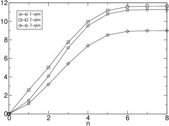
Figure 3: RG flow of on-site fields at temperature $T/J=0.5$ for $p=3$ and $M=3$. Circles, squares and diamonds correspond to the one-spin, two-spin and three-spin one-site terms, respectively.

We now study how the standard deviations of couplings behave as a function of the length scale $L=2^{n}$. The standard deviation $K$ of the three-spin couplings shown in Fig. 1 decays as $\exp(-L/\xi(T))$, where $\xi(T)$ at temperature $T$ can be interpreted as the correlation length. In Fig. 4, the correlation lengths of the two 3-spin glass models with $M=2$ and $M=3$ are shown. The correlation length for the $p=3$, $M=2$ model has been already obtained in Ref. MD . The $M=3$ model has longer correlation length than the $M=2$ model at any given temperature. The correlation lengths of the two models basically show the same temperature dependence. They increase quite rapidly as the temperature is lowered and then saturate at large values in the zero temperature limit.

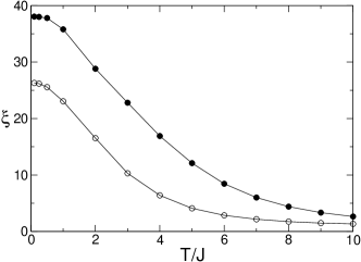
Figure 4: Correlation length $\xi$ as a function of temperature $T/J$ for the $p=3,M=3$ model (filled circles) and the $p=3,M=2$ model (open circles).

In summary, we have investigated the RG flows of the coupling constants in the $M$-$p$-spin glass model with $p=3$ and $M=3$ in three dimensions using the Migdal-Kadanoff approximation. All the coupling constants flow to the high temperature sink implying that there is no finite temperature phase transition in this model. The correlation length increases quite rapidly as the temperature is lowered and saturates in the zero temperature limit. All these features are very similar to those of its $M=2$ counterpart. The only difference is that the $M=3$ model has longer correlation lengths. This is quite remarkable in that the two models show completely different behavior at the mean-field level. Therefore we conclude that in the $3$-spin spin glass models, thermal fluctuations in three dimensions completely destroy the transitions predicted by mean-field theory: whether $R>1$ or is less than $1$ results in only a quantitative change in the magnitude of the correlation length.

What stimulated this investigation was the renormalization group analysis by Cammarota et al. CBTT of a replicated Hamiltonian similar to $\mathcal{H}_{\mathrm{GLW}}$ in Eq. (2). Like us they used a MK approximation appropriate to three dimensions, but instead found a transition which they identified as the transition expected in random first-order transition theory KTW at a temperature they identified as $T_{K}$. We believe the difference in results stems from their decimation step in the MK procedure. In our work it is carried out exactly. In the calculation of Ref. CBTT , however, it was done by a steepest-descent approximation to an integral over $n\times n$ replica matrices, and the magnitude of the corrections to this approximation were not assessed. They themselves suggested that the calculations actually done in this paper should be carried out as a check of their decimation approximation. Our calculations alas provide no support for it.

JY was supported by WCU program through the KOSEF funded by the MEST (Grant No. R31-2008-000-10057-0).

References

- (1) T. R. Kirkpatrick and P. G. Wolynes, Phys. Rev. A 35, 3072 (1987); T. R. Kirkpatrick and D. Thirumalai, Phys. Rev. B 36, 5388 (1987); T. R. Kirkpatrick and P. G. Wolynes, Phys. Rev. B 36, 8552 (1987).
- (2) W. Götze and L. Sjögren Rep. Prog. Phys 55241 (1992); W. Götze in Liquid, Freezing and the Glass Transition, edited by J. P. Hansen, D. Levesque and J. Zinn-Justin, (Elsevier, New York, 1991); J. P. Bouchaud, L. F. Cugliandolo, J. Kurchan and M. Mezard in Spin Glasses and Random Fields, edited by A. P. Young, (World Scientific, Singapore, 1997).
- (3) W. Kauzmann, Chem. Rev. 43, 219 (1948).
- (4) G. Parisi, M. Picco and F. Ritort, Phys. Rev. E 60, 58 (1999).
- (5) F. Caltagirone, U. Ferrari, L. Leuzzi, G. Parisi and T. Rizzo, Phys. Rev. B 83 204202 (2011).
- (6) B. Drossel, H. Bokil and M. A. Moore, Phys. Rev. E 62, 7690 (2000).
- (7) M. A. Moore and B. Drossel, Phys. Rev. Lett. 89, 217202 (2002).
- (8) M. A. Moore and A. J. Bray, Phys. Rev. B 83, 224408 (2011).
- (9) D. Larson, H. G. Katzgraber, M. A. Moore and A. P. Young, Phys. Rev. B 81, 064415 (2010).
- (10) D. J. Gross, I. Kanter, and H. Sompolinsky, Phys. Rev. Lett. 55, 304 (1985).
- (11) C. Cammarota, G. Biroli, M. Tarzia, and G. Tarjus, Phys. Rev. Lett. 106, 115705 (2011).