Optical surface modes in the presence of nonlinearity and disorder

Abstract

We investigate numerically the effect of the competition of disorder, nonlinearity, and boundaries on the Anderson localization of light waves in finite-size, one-dimensional waveguide arrays. Using the discrete Anderson - nonlinear Schrödinger equation, the propagation of the mode amplitudes up to some finite distance is monitored. The analysis is based on the calculated localization length and the participation number, two standard measures for the statistical description of Anderson localization. For relatively weak disorder and nonlinearity, a higher disorder strength is required to achieve the same degree of localization at the edge than in the interior of the array, in agreement with recent experimental observations in the linear regime. However, for relatively strong disorder and/or nonlinearity, this behavior is reversed and it is now easier to localize an excitation at the edge than in the interior.

Introduction.- A fundamental question concerning systems which are both disordered and nonlinear is whether or not Anderson localization Anderson1958 is weakened by the presence of nonlinearity. While it was originally developed in order to understand electronic transport in non-periodic (disordered) solids, the concept of Anderson localization was later generalized to the localization of classical waves in disorder media John1987 . The interaction of propagating waves, and in particular of electromagnetic waves, when both disorder and nonlinearity are present can significantly affect localization and other phenomena Bishop1989 .

Despite of many efforts, that question has not been conclusively answered Molina1998 ; Kopidakis2000 ; Kopidakis2008 ; MVK ; Kivshar1990 ; Pikovsky2008 ; Flach2009 ; Fishman2011 . It thus seems that the answer depends on the relative strength of disorder and nonlinearity. For large nonlinearity, time-periodic and exponentially localized excitations in the form of discrete breathers may be generated, due to the self-trapping effect Molina1993 . For small disorder strength, the discrete breathers are modulated to become localized modes Ivanchenko2009 . The above theoretical results were accompanied by a series of experimental demonstrations of Anderson localization in optics Pertsch2004 and Bose-Einstein condensates Billy2008 .

It was recently observed experimentally that Anderson localization in finite segments of disordered waveguide arrays in the linear regime is actually site-dependent Szameit2010 . Specifically, a higher disorder strength is required to achieve the same degree of localization at the edge than in the interior (i.e., the ”bulk”) of the array Szameit2010 . Here we are interested in the effect of the interplay of disorder and nonlinearity on the site-dependence of wavepacket localization in one-dimensional (1D), disordered, finite-size arrays of coupled Kerr-type waveguides. Using the discrete nonlinear Schrödinger (DNLS) equation with diagonal (on-site) disorder, frequently referred to as the discrete Anderson - nonlinear Schrödinger (DANLS) equation, we calculate standard measures of Anderson localization in order to analyze the site-dependence of the degree of localization for a wide range of nonlinearity and disorder strengths.

Model equations and statistical measures.- Consider a 1D array of $N$ single-mode optical waveguides. In the framework of the coupled-modes formalism, the electric field $C(x,z)$ propagating along the waveguides can be expanded as a superposition of the waveguide modes, $C(x,z)=\sum_{n}C_{n}(z)\phi(x-n)$, where $C_{n}$ is the complex amplitude of the single guide mode $\phi(x)$ centered at the $n$th site. The evolution equations for the modal amplitudes $C_{n}$ are

$$i\frac{dC_{n}}{dz}+V_{n,n-1}C_{n-1}+\epsilon_{n}C_{n}+V_{n,n+1}C_{n+1}+\chi|C_{n}|^{2}C_{n}=0,$$ (1)

where $n=1,2,3,...,N$, $\epsilon_{n}$ is the propagation constant associated with the $n$th site, $V_{n,n\pm 1}$ are the tunneling rates between two adjacent sites, $\chi$ is the nonlinearity parameter, and $z$ is the spatial coordinate along the propagation direction (‘time’). Eq. (1) describes very well recent experiments in 1D disordered waveguide lattices and, moreover, it serves as a paradigmatic model for a wide class of physical problems where both disorder and nonlinearity are important. Disorder is introduced into the optical lattice by randomly choosing the propagation constants $\epsilon_{n}$ from a uniform, zero-mean distribution in the interval $[-\Delta,+\Delta]$. As a result, the lattice remains periodic on average and, to a very good approximation, the parameters $V_{n,n\pm 1}$ become independent of the site number $n$, i.e., $V_{n,n\pm 1}=V$. Then, Eq. (1) reads

$$i\frac{dC_{n}}{dz}+\epsilon_{n}C_{n}+V(C_{n-1}+C_{n+1})+\chi|C_{n}|^{2}C_{n}=0.$$ (2)

In order to take into account the termination of the structure, we impose free boundary conditions at the edges, i.e., $C_{0}=C_{N+1}=0$. For $\chi\rightarrow 0$, Eq.(2) reduces to the original Anderson model while in the absence of disorder ($\epsilon_{n}=0$), it reduces to the 1D DNLS equation Kevrekidis2009 that is generally non-integrable and it conserves the norm ${\cal N}=\sum_{n=1}^{N}|C_{n}|^{2}$ and the Hamiltonian $\cal{H}$.

To investigate the simultaneous interplay of disorder, nonlinearity and boundary effects, we place initially a single-site excitation $C_{n}=\delta_{n,n_{0}}$ near, or at the boundary of the array. This determines the value of the norm ${\cal N}=1$ for all subsequent ‘times’. For a quantitative analysis we utilize two of the standard measures used in the description of Anderson localization; the participation number $P=\left\{\sum_{n=1}^{N}|C_{n}|^{4}\right\}^{-1}$ , and the localization length $\ell$, defined as the width of the envelope containing the localized profile. The participation number gives a rough estimate of the number of sites where the wavepacket has significant amplitudes, and it is a useful measure for ascertaining localization effects in the case of partial localization. In this case, $P$ will saturate at a finite value, indicating the formation of a localized wavepacket.

Statistical analysis.- In the following, we set $V=1$, while the nonlinearity parameter $\chi$ varies between $0$ and $10$, and the disorder width $\Delta$ takes on several different values. Since Anderson localization is essentially a statistical phenomenon, many realizations of disorder are needed to obtain meaningful averages for the quantities of interest. This is particularly true for low-dimensional systems. We typically use $n_{R}=1000$ realizations in each run. The array contains $N=200$ waveguides, and the maximum evolution “time” is $z=100$ (except otherwise stated). In optics, nonlinearity is varied by changing the power content of the input beam. However, this is formally equivalent to keeping the norm of the wavepacket fixed, and to varying the nonlinearity parameter $\chi$. Eqs. (2) are integrated with a standard 4rth order Runge-Kutta algorithm with fixed time-stepping. We compute the absolute squared profiles $<|C_{n}|^{2}>$, where the brackets denote averaging over all realizations $n_{R}$, hereafter referred to as Anderson mode profiles. Assuming that the Anderson modes have a $z-$dependence which is a simple exponential function of the form $<|C_{n}|^{2}>=C_{max}^{2}\,e^{-z/\ell}$, the localization length $\ell$ can be computed via $\chi^{2}$ fitting procedure, with $C_{max}^{2}$ being the numerically obtained maximum of $<|C_{n}|^{2}>$.

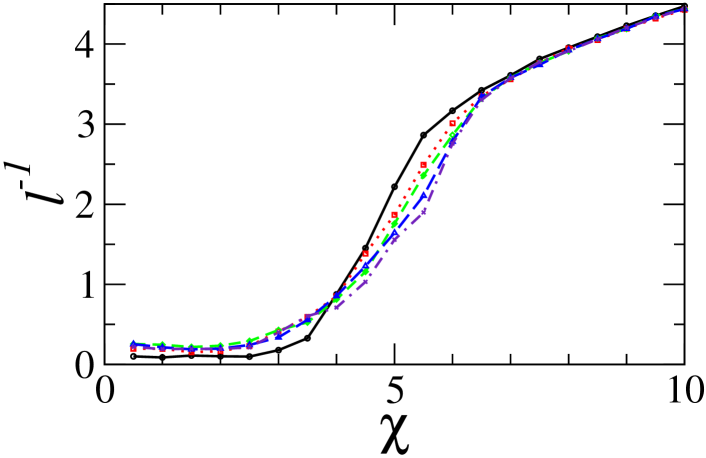
Figure 1: (color online) Inverse localization length $\ell^{-1}$ as a function of the nonlinearity strength $\chi$. A single-site excitation is launched from $n_{0}=1$ (solid - black), 2 (red - dotted), 3 (green - dashed), 5 (blue - long-dashed), 10 (indigo - dotted-dashed), for a system with $N=200$, $V=1$, $z=100$, $n_{R}=1000$, and $\Delta=0.6$.

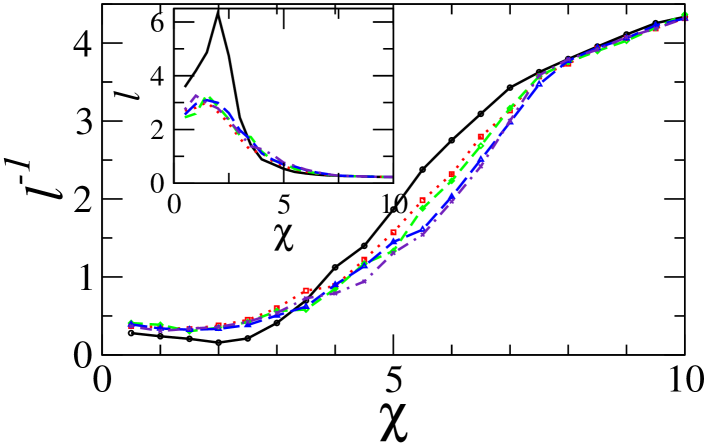
Figure 2: (color online) Inverse localization length $\ell^{-1}$ and localization length $\ell$ (inset) as a function of the nonlinearity strength $\chi$. Same parameters and notation as in Fig. 1, but $\Delta=1.0$.

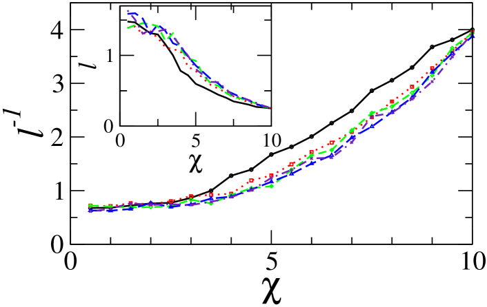
Figure 3: (color online) Inverse localization length $\ell^{-1}$ and localization length $\ell$ (inset) as a function of the nonlinearity strength $\chi$. Same parameters and notation as in Fig. 1, but $\Delta=2.0$.

In Figs. 1-3 the inverse localization length $\ell^{-1}$ is shown as a function of $\chi$ for three different values of disorder strength. In all the cases displayed in these figures the initial wavepacket is a single-site excitation placed at $n=n_{0}$, with $n_{0}=1$ (right at the edge), 2, 3, 5, and 10. In Fig. 1 (where $\Delta=0.6$) we easily identify two different $\chi-$ regimes; the weak and the strong nonlinearity regime, where $\ell^{-1}$ is small and large, respectively. That generaly implies a lower degree of Anderson localization in the weak nonlinearity regime compared to that in the strong nonlinearity regime. The large $\ell^{-1}$ in the interval of $\chi$ values where all the curves fall the one onto the other, indicates the existence of a highly localized mode due to the self-trapping effect. The characteristic nonlinearity strength, $\chi_{c}$, that roughly distinguishes between the two regimes is the critical on for self-trapping to occur in the 1D DNLS equation Molina1993 . In the weak nonlinearity regime another important feature appears; as it can be seen in the figure, the $\ell^{-1}(\chi)$ curve obtained for excitations initially placed at the edge ($n_{0}=1$) is well below all the others (for which $n_{0}>1$). Thus, an excitation initially placed at the edge ($n_{0}=1$) leads to final wavepackets that are less localized than those which have been initialized below the ’surface’ ($n_{0}>1$). This effect can be understood as the ”repulsive” action of the boundary, reported in a previous work for surface modes in nonlinear periodic lattices MVK , and it is in agreement with the experimental observations of Ref. Szameit2010 .

As the disorder strength $\Delta$ is increased from $0.6$ to $1.0$ (Fig. 2), all the curves become flatter without showing any qualitative difference from those of Fig. 1. When $\Delta$ is increased to $2.0$, however, we do observe qualitative differences (Fig. 3). For weak nonlinearity ($\chi\stackrel{{\scriptstyle<}}{{\sim}}4\sim\chi_{c}$) there are no significant differences in the degree of localization for the Anderson modes resulting from initial excitations either at the edge or in the interior of the array. Thus, it is as easy to localize a wavepacket at the edge as it is in the interior in this case. However, for intermediate nonlinearities (from $\chi\stackrel{{\scriptstyle>}}{{\sim}}4$ to $\chi\simeq 8$) it is more favorable to loacalize a wavepacket at the edge than in the bulk, whereas for large nonlinearities $\chi\stackrel{{\scriptstyle>}}{{\sim}}8$ it is as easy to localize a wavepacket at the edge as it is in the bulk. Thus, for relatively strong disorder we observe a bahavior that is strikingly different to what is observed in Figs. 1 and 2. The two different behaviors can be seen even more clearly by comparison of the localization length $\ell$ as a function of $\chi$ for $\Delta=1$ and $2$, shown in the insets of Fig. 2 and 3, repsectively. Thus, the presence of strong disorder is capable of overcoming the ”repulsive” character of the boundary for any value of $\chi$ and, moreover, it favors wavepacket localization at the edges for intermediate nonlinearities.

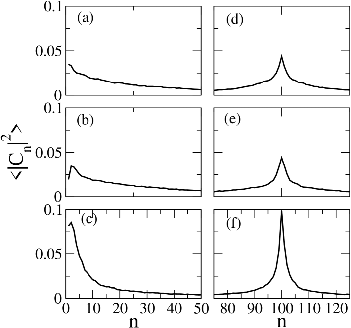
Figure 4: Anderson mode profiles $<|C_{n}|^{2}>$ as a function of the site-number $n$ for $N=200$, $V=1$, $\Delta=0.6$, $z=1000$, $n_{R}=1000$, and $\chi=1$ (a,d), $\chi=2$ (b,e) and $\chi=3$ (c,f). Left panels denote the surface mode case ($n_{0}=1$) while right panels refer to the bulk mode case ($n_{0}=100$). Only part of the array sites are shown for clarity.

Typical examples of localized mode profiles both at, or close to the edge and the ’bulk’ are shown in Fig. 4, where the Anderson mode profiles $<|C_{n}|^{2}>$ are shown as a function of $n$ for $\Delta=0.6$. (Note that in this figure $z=1000$.) The edge-localized modes are significantly more extended than the bulk modes, even though the former are not all localized exactly at the edge. This is because of the small disorder strength $\Delta$, which allows the repulsive force of the boundary on the mode to dominate and move slightly the mode-maximum towards the bulk. However, similar profiles (not shown) are obtained also for $\Delta=1.0$, that is large enough to keep the localized modes at their initial location.

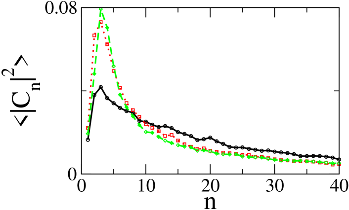
Figure 5: (color online) Averaged absolute squared profiles $<|C_{n}|^{2}>$ as a function of the site-number $n$ for $N=200$, $V=1$, $\Delta=0.4$, $n_{R}=1000$, $\chi=2.5$, $z=100$. These profiles result from a single-site initial excitation at $n_{0}=1$ (black-solid); $n_{0}=2$ (red-dotted); $n_{0}=3$ (green-dashed). Only part of the array sites are shown for clarity.

Moreover, single-site excitations initialized at different sites $n_{0}$ can be pushed by the boundary towards the interior and form Anderson modes at the same final site. These modes are different, at least for finite propagation distances $z$; they differ in the degree of localization, leading to a multiplicity of Anderson modes having their maximum at the same site of the lattice (Fig. 5). For the particular value of $\chi$ used for Fig. 5, three single-site excitations initialized at different $n_{0}$ have formed, after they have been propagated up to $z=100$, three distinct Anderson localized modes whose maximum is located at the same lattice site (i.e., at $n=3$).

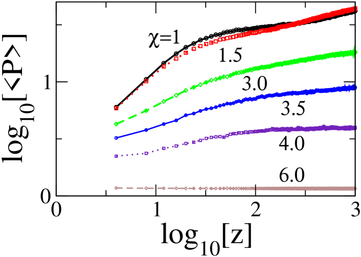
Figure 6: (color online) Logarithm of the averaged participation number $\log_{10}(<P>)$ as a function of $\log_{10}(z)$ for the surface case ($n_{0}=1$) and $N=200$, $V=1$, $\Delta=0.6$, $n_{R}=1000$, $z=1000$. The values of $\chi$ are shown on the figure.

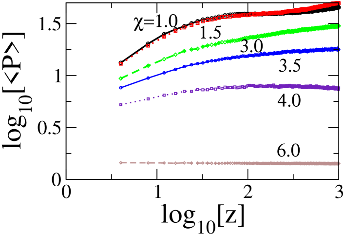
Figure 7: (color online) Logarithm of the averaged participation number $\log_{10}(<P>)$ as a function of $\log_{10}(z)$ for the bulk case ($n_{0}=100$) and $N=200$, $V=1$, $\Delta=0.6$, $n_{R}=1000$, $z=1000$, $n_{0}=100$. The values of $\chi$ are shown on the figure.

Finally, let us look at the participation number $P$ as a function of $z$ for wavepackets that are initially localized at the edge ($n_{0}=1$) and in the ’bulk’ ($n_{0}=100$) of the waveguide array. The logarithmic plots are shown in Fig. 6 and Fig. 7, respectively, for several values of $\chi$ and weak disorder. Comparing the curves in these figures corresponding to the same $\chi$, we see that those for $n_{0}=100$ are shifted to higher $P$ values than those for $n_{0}=1$. Thus, single-site excitations initialized at $n_{0}=100$ have, while propagating along $z$, a larger number of sites where the wavepacket has significant amplitudes. However, the excitations initialized at $n_{0}=100$ exhibit a higher degree of localization than those initialized at $n_{0}=1$ (see also Fig. 4). It is also interesting to see how the curves in each figure change as a function of $\chi$. For $\chi=6$, well above $\chi_{c}$, we see that the wavepacket remains localized at a single site, independently of $n_{0}$. For $\chi=4\sim\chi_{c}$, the $\log_{10}(<P>)$ vs. $\log_{10}(z)$ curve increases slowly with increasing $\log_{10}(z)$, and it saturates at a finite value around $z\simeq 100$, indicating the formation of a wavepacket highly localized around $n_{0}$. For the nonlinearity strengths that are less than $\chi_{c}$, the $\log_{10}(<P>)$ vs. $\log_{10}(z)$ curves exhibit qualitatively the same behavior. There is an increase with increasing $\log_{10}(z)$ which is slowed down after some $z$ specific to each $\chi$ value, and indicates significant delocalization of the initially single-site wavepacket. Delocalization is stronger for decreasing nonlinearity strength. However, those curves do not seem to saturate, implying that the corresponding Anderson localized modes may delocalize further at longer propagation distances.

Concluding remarks.- We have performed extensive calculations with the 1D DANLS equation in order to clarify some aspects of the interplay between boundary effects, disorder and nonlinearity, in finite-size waveguide arrays. In particular, we attempt to clarify the site-dependence of Anderson localization that results from that interplay. We computed two standard measures of localization for discrete systems for varying nonlinearity and disorder strengths, and we observed two strikingly different behaviors depending on the strength of the disorder. For weak to moderate disorder, we distinguish two different nonlinearity regimes; weak and strong, for values of $\chi$ roughly below and above $\chi_{c}$, respectively. In the weak nonlinearity regime it is easier to localize a wavepacket in the interior of the array than at the edge, which is in agreement with the experiments in the linear regime Szameit2010 . In the strong nonlinearity regime it is as easy to localize a wavepacket at the edge as it is in the interior. However, for relatively strong disorder, this behavior is reversed, at least for intermediate nonlinearities, and it is now easier to localize a wavepacket at the edge than in the bulk. For weak and very strong nonlinearities there is no significant site-dependence on the degree of wavepacket localization. The results presented here obviously hold for finite propagation distance $z$, an important case of practical interest for experimentalists.

Acknowledgements.- M.I.M. acknowledges support from Fondecyt Grant 1080374 and Programa de Financiamiento Basal de Conicyt (Grant No. FB0824/2008)

References

- (1) P. W. Anderson, Phys. Rev. 109, 1492 (1958).
- (2) S. John, Phys. Rev. Lett. 58, 2486 (1987).
- (3) Disorder and Nonlinearity, edited by A. R. Bishop, D. K. Campbell, and St. Pnevmatikos (Springer-Verlag, Berlin, 1989); Nonlinearity with Disorder, edited by F. Kh. Abdullaev, A. R. Bishop, and St. Pnevmatikos (Springer-Verlag, Berlin, 1991).
- (4) M. I. Molina, Phys. Rev. B 58, 12547 (1998).
- (5) G. Kopidakis and S. Aubry, Phys. Rev. Lett. 84, 3236 (2000).
- (6) G. Kopidakis et al., Phys. Rev. Lett. 100, 084103 (2008).
- (7) M. I. Molina. R. A. Vicencio, and Y. S. Kivshar, Opt. Lett. 31, 1693 (2006).
- (8) Yu. S. Kivshar et al., Phys. Rev. Lett. 64, 1693 (1990).
- (9) A. S. Pikovsky and D. L. Shepelyansky, Phys. Rev. Lett. 100, 094101 (2008).
- (10) S. Flach, D. O. Krimer, and Ch. Skokos, Phys. Rev. Lett. 102, 024101 (2009).
- (11) S. Fishman, Y. Krivolapov, and A. Soffer, arXiv:1108.2956v1 [math-ph].
- (12) M. I. Molina and G. P. Tsironis, Physica D 65, 267 (1993); M. I. Molina and G. P. Tsironis, Int. J. of Mod. Phys. B 9, 1899 (1995).
- (13) M. V. Ivanchenko, Phys. Rev. Lett. 102, 175507 (2009).
- (14) T. Pertsch et al., Phys. Rev. Lett. 93, 052901 (2004); T. Schwartz et al., Nature 446, 52 (2007); Y. Lahini et al., Phys. Rev. Lett. 100, 013906 (2008).
- (15) J. Billy et al., Nature 453, 891 (2008); G. Roati et al., Nature 453, 895 (2008).
- (16) A. Szameit et al., Opt. Lett. 35, 1172 (2010).
- (17) P. G. Kevrekidis, The Discrete Nonlinear Schrödinger Equation, Springer-Verlag, Berlin, Heidelberg (2009).