Electron spin resonance study of anisotropic interactions in a two-dimensional spin gap magnet PHCC

Abstract

Fine details of the excitation spectrum of the two-dimensional spin-gap magnet PHCC are revealed by electron spin resonance investigations. The values of anisotropy parameters and the orientations of the anisotropy axes are determined by accurate measurements of the angular, frequency-field and temperature dependences of the resonance absorption. The properties of a spin-gap magnet in the vicinity of critical field are discussed in terms of sublevel splittings and $g$-factor anisotropy.

I Introduction

Piperazinium hexachlorodicuprate (C₄H₁₂N₂)(Cu₂Cl₆), abbreviated as PHCC, was studied recently as a good test example of a two-dimensional Heisenberg antiferromagnet.broholm-njp2007 ; broholm-prb64 ; stone-nature Inelastic neutron scattering experiments revealed that each magnetic ion interacts with at least six in-plane neighbours. The strongest exchange integral value is approximately 1.3 meV. The complex geometry of the exchange bonds can be envisioned as a set of strongly coupled antiferromagnetic ladders running along the $\mathbf{a}$ axis (from here on we use the axes notation of Ref.structure, ) of the triclinic crystal while some of the weaker exchange bonds are frustrated.broholm-prb64 The magnetic ground state of PHCC is a non-magnetic singlet separated from the excited triplet states by an energy gap of $\Delta=1.02$ meV. broholm-njp2007

Due to the presence of the gap PHCC remains in the disordered spin-liquid state down to temperatures well below the exchange integral scale. At low temperatures the magnetic properties of this system can be considered as those of a gas of weakly-interacting triplets. The application of an external field lowers the energy of one of the triplet substates and, at a certain critical field, a quantum phase transition to a field-induced antiferromagnetic state occurs. The closing of the gap and the formation of magnetic order above the critical field of $\approx 8$ T was confirmed by magnetic measurements as well as by calorimetric and neutron scattering techniques broholm-njp2007 . Additionally, this magnet was used as a test probe for the quasiparticle breakdown in a quantum spin liquid stone-nature .

Magnetization measurements revealed an anisotropy of the critical field broholm-njp2007 . This anisotropy points to deviations from the Heisenberg model. Such deviations are important for the physics of a spin-gap magnet, especially around the quantum phase transition. Anisotropic interactions are known to cause a gap reopening in fields above the phase transition and they could also affect the quasiparticle decay by allowing otherwise forbidden processes.

In this paper we present results of electron spin resonance (ESR) investigations of PHCC. Our study reveals the presence of anisotropic interactions leading to a $g$-factor anisotropy and a splitting in the triplet sublevels. We have determined magnitudes of these anisotropic effects and the orientations of the corresponding axes. Additionally, we address the question of the correct implementation of a macroscopic theory Affleck ; farmar to the case of a spin-gap magnet with a relevant $g$-factor anisotropy.

II Experimental details and samples

The samples were grown from saturated solutions of PHCC. The saturated solution was prepared by adding of piperazine C₄H₁₀N₂ (from Sigma Aldrich), dissolved in minimal amount of concentrated HCl to CuCl${}_{2}\cdot 2$H₂O (99.99% purity from Sigma Aldrich), dissolved in minimal amount of concentrated HCl, at a 4:1 molar ratio of CuCl₂ to C₄H₁₀N₂.

The main set of samples for the ESR measurements was grown by cooling the filtered saturated solution in the refrigerator. After several days numerous as-grown crystals have appeared and were naturally shaped as flat parallelograms of transparent orange-brown color. The typical sample size was $3-5$ mm along the longest side of the parallelogram. The crystallographic symmetry was checked by X-ray diffraction and found to be triclinic with lattice parameters and angles in agreement with the literature structure . The plane of the as-grown crystals was perpendicular to the $\mathbf{a}^{*}$ axis of the reciprocal lattice. The long and short side of the parallelogram was parallel to the $\mathbf{c}$ and the $(\mathbf{b}+\mathbf{c})$ direction, respectively. This natural shape of the crystals allowed an easy orientation of the crystals in the magnetic field $\mathbf{H}$ with $\mathbf{H}||\mathbf{a}^{*}$, $\mathbf{H}\perp\{\mathbf{a}^{*},\mathbf{c}\}$ or $\mathbf{H}\perp\{\mathbf{a}^{*},(\mathbf{b}+\mathbf{c})\}$.

Additionally, a larger sample was grown from the seed by a temperature gradient method. This sample has a well developed plane normal to the $\mathbf{a}^{*}$ axis and has its longest dimension parallel to $\mathbf{c}$-axis. For reasons related to the sample space configuration this sample was used for measurements with $\mathbf{H}||\mathbf{a}^{*}$ and $\mathbf{H}\perp\{\mathbf{a}^{*},\mathbf{c}\}$ only. Samples of deuterated PHCC used for the specific heat measurements were grown from the seed in a similar way.

The samples were characterized by static magnetization measurements with a Quantum Design MPMS system. The concentration of impurities was estimated from the low-temperature susceptibility assuming $g=2.0$ and $S=1/2$ and was less than $4\times 10^{-4}$ paramagnetic impurities per copper ion.

The technique of electron spin resonance is a powerful tool for the study of low energy dynamics of a spin-gap magnet. It can access inter-triplet transitions and measures directly the differences between triplet sublevels. Characteristic orientational, frequency-field and temperature dependences of the resonance absorption spectra provide information on anisotropic interactions, zero field splittings and the $g$-factor anisotropy.

In case of PHCC additional complications and challenges arise from the low (triclinic) symmetry of the crystals. Due to this low symmetry, neither the $g$-tensor nor the anisotropy tensor are fixed to any of the crystal axes. This means that the axes orientation for all anisotropic contributions should be considered as arbitrary and mutually independent. To solve this problem we have taken a series of absorption spectra at different temperatures and at different orientations of the applied magnetic field.

The ESR measurements were carried out in the frequency range from 9GHz to 120GHz and at temperatures down to 0.4 K. X-band (9.4 GHz) measurements above $T=2.5$ K were done with a Bruker EleXsys spectrometer equipped with a He-flow type cryostat and an automated sample goniometer. For higher frequency measurements a set of homemade transmission type ESR spectrometers equipped with $6-8$ T cryomagnets and microwave oscillators covering the frequency range up to 120 GHz were used. Measurements below 1 K were performed with a home made ESR spectrometer equipped with ³He-pumping cryostat and a 12 T cryomagnet.

Low-temperature specific heat measurements in an applied magnetic field up to 14 T were performed with a Quantum Design PPMS system equipped with a dilution refrigerator.

III Experimental results

III.1 Temperature evolution of ESR spectra

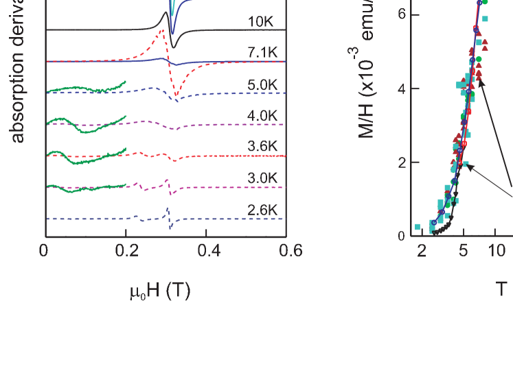
Figure 1: (color online) Left panel: Temperature evolution of X-band ESR absorption derivative (arb. units, $f=9.4$ GHz, orientation close to $\mathbf{H}\perp\{\mathbf{a}^{*},\mathbf{c}\}$). Dashed lines are y-magnified by a factor of 10 with respect to the raw data. Low-field part of low-temperature absorption curves is y-magnified by a factor of 100 with respect to the raw data. Right panel: Temperature dependence of the static susceptibility (filled circles, denoted as ”SQUID”) and integrated intensity of ESR absorption (filled squares, denoted as ”X-band”, from the analysis of absorption at the frequency of $9.4$ GHz; other symbols, denoted as ”38 GHz”, from the analysis of absorption in different orientations at frequencies close to 38 GHz).

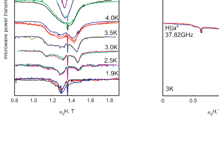
Figure 2: (color online) Left panel: Temperature dependence of ESR absorption ($f=38.04$ GHz, $\mathbf{H}||\mathbf{a}^{*}$). Right panel: ESR absorption spectra for different orientations at 3.0 K.

The temperature evolution of the ESR absorption is illustrated in Figures 1 and 2. At high temperatures we observe a single-component ESR absorption with a $g$-factor close to 2, which is typical for Cu²⁺ ions. Below approximately $10-15$ K the intensity of the resonance quickly decreases. As expected for a spin-gap magnet this decrease can be scaled with the decrease of the static susceptibility (see right panel of Figure 1).

As the intensity of the absorption decreases with cooling the absorption line broadens and, around 5 K, it splits into several components. This splitting is anisotropic (see right panel of Figure 2). One can distinguish several components that continue to fade out with cooling and one component, located close to a $g=2.0$ resonance field, with an increasing intensity upon cooling. The fading components can be ascribed to a resonance of triplet excitations, while an irregularly shaped component with increasing intensity corresponds to defects and impurities.

The magnitude of the splitting is temperature dependent but appears almost constant for temperatures lower or equal to 3 K (see Figures 1 and 2). Because of the rapid decrease of intensity of the split spectral features below 3 K we performed all measurements for the determination of the splitting parameters at 3 K.

III.2 Frequency-field diagrams

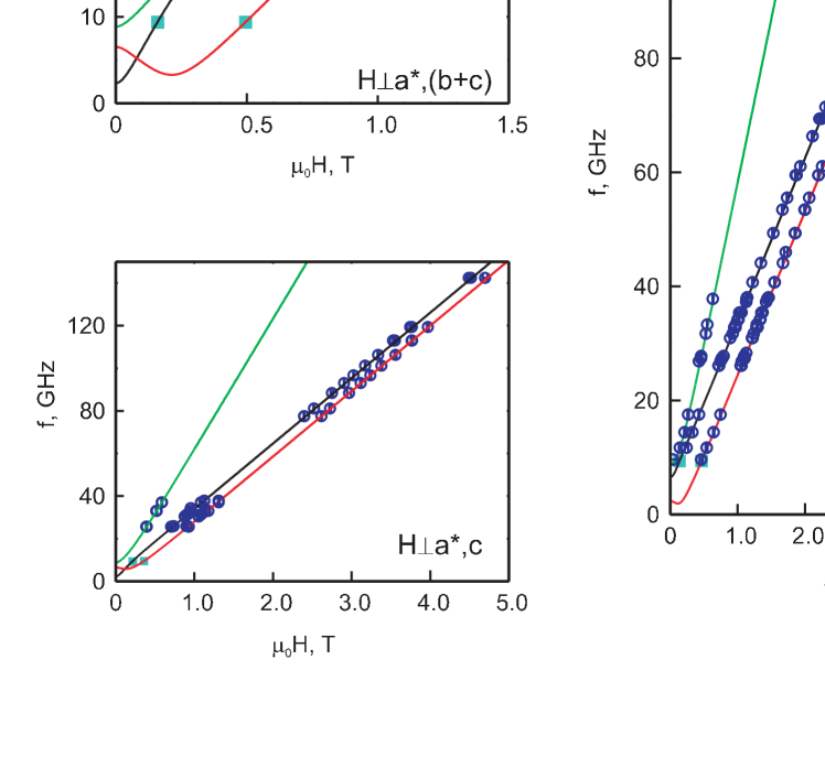
Figure 3: (color online) Frequency field diagrams for different orientations of the applied field at $T=3.0$ K. Open circles: high frequency measurements at fixed orientations. Closed squares: resonance field positions for corresponding orientations extracted from X-band (9.4GHz) orientational dependences. Curves: perturbative model calculations.

Above the splitting temperature where the ESR absorption consists of a single component the measurements at different frequencies proved that the resonance field can be described by an effective $g$-factor: for $\mathbf{H}||\mathbf{a}^{*}$ $g=2.05\pm 0.01$, for $\mathbf{H}\perp\{\mathbf{a}^{*},\mathbf{c}\}$ $g=2.206\pm 0.002$ and for $\mathbf{H}\perp\{\mathbf{a}^{*},(\mathbf{b}+\mathbf{c})\}$ $g=2.236\pm 0.002$.

Frequency-field diagrams for the resonance fields measured at 3.0K are shown on the Figure 3. For all three chosen orientations the two main absorption components are located to the left and to the right of the high-temperature resonance position. Another, weaker component located at approximately half of the first resonance field (see also right panel of Figure 2) was observed in the measurements with the larger sample for $\mathbf{H}||\mathbf{a}^{*}$ and $\mathbf{H}\perp\{\mathbf{a}^{*},\mathbf{c}\}$. The slope of the main components is determined by corresponding $g$-factor value. The splitting of these components is orientation dependent and is equal to 9.2 GHz, 5.5 GHz and 12.8 GHz for $\mathbf{H}||\mathbf{a}^{*}$, $\mathbf{H}\perp\{\mathbf{a}^{*},\mathbf{c}\}$ and $\mathbf{H}\perp\{\mathbf{a}^{*},(\mathbf{b}+\mathbf{c})\}$, correspondingly.

III.3 Orientational dependences

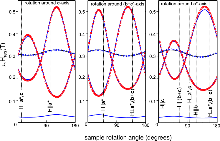
Figure 4: (color online) Orientational dependences of resonance field in X-band (9.4 GHz) experiments. Selected field directions with respect to the crystal axes are shown as determined from the fit. Circles, squares: experimental data at 25 K and 3.0 K, respectively. Lines: best fit by the perturbative model described in the text.

The angular dependences of the ESR absorption were accurately measured at X-band frequency (9.4 GHz) for $T=3.0$ K (below the splitting temperature) and for $T=25$ K (above the splitting temperature) where the linewidth shows a minimum. Three non-orthogonal rotation axes were chosen for different experiments, namely rotations around the $\mathbf{a}^{*}$ reciprocal space axis, around the $\mathbf{c}$ axis and around the $(\mathbf{b}+\mathbf{c})$ direction. The samples were fixed with paraffine inside suprasil glass tubes, with the chosen rotation axis parallel to the tube axis. The accuracy of this sample mounting technique was limited with respect to the rotations around the tube axis and, thus, the unavoidable angle shift was later taken as a fit parameter.

The positions of the resonance fields shown in Figure 4 were determined from fitting the spectra by a single or a multi-component absorption, assuming a Lorentzian shape for each of the components. For the data at 3.0 K we did not include the weak low-field component (see the line below 0.2 T in the left panel of Fig. 1), since this line is broad and distorted in shape, which makes a precise determination of the resonance field unreliable.

III.4 Low temperature ESR measurements

To check for possible singlet-triplet transitions and antiferromagnetic resonance in the field-induced ordered phase we performed additional measurements at the temperatures down to 450 mK using the large sample with $\mathbf{H}\|\mathbf{a}^{*}$. At frequencies of 27 GHz and 33 GHz and for fields up to 12T we did not observe any other resonance absorption at 450 mK besides that due to defects. On heating above 1.5 K a split ESR absorption, similar to that described in the above subsections, was observed.

III.5 Critical field measurements

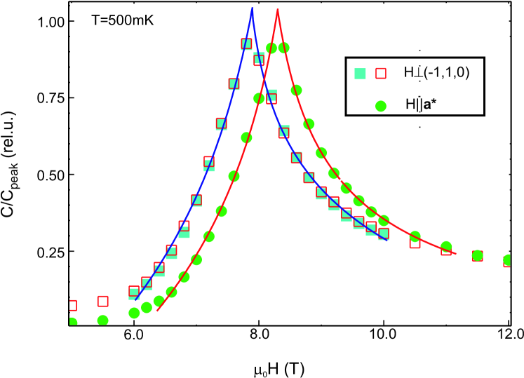
Figure 5: (color online) Field dependences of the specific heat of deuterated PHCC at different orientations and at $T=0.5$ K. Curves are guides to the eye.

In order to determine the critical fields at different orientations the field dependence of the specific heat was measured at 500 mK (Figure 5). These measurements were done on deuterated samples of PHCC while non-deuterated samples were used for ESR experiments. A sharp maximum of the specific heat marks the transition to the field-induced ordered phase. The determined values of the critical fields are: for $\mathbf{H}||\mathbf{a}^{*}$ $\mu_{0}H_{c}=8.29\pm 0.05$T, for $\mathbf{H}\perp(-1,1,0)$ $\mu_{0}H_{c}=7.90\pm 0.07$T.

IV Discussion

This section is built as follows: first, we will qualitatively describe our data and will show that our observations reflect the effects of anisotropic interactions; second, we will make a quantitative analysis of the ESR data and will estimate the strength of these anisotropic interactions; finally, we will discuss the relations between the found anisotropic properties at low field with the known anisotropic properties at the critical field.

IV.1 Qualitative description

The observed evolution of the ESR absorption spectra is typical for a spin-gap magnet with triplet levels split by an effective crystal field. A similar behaviour was observed earlier for other spin-gap magnets, e.g. TlCuCl₃ glazkov-tlcucl3 and NTENP glazkov-ntenp .

The decrease of the absorption intensity with temperature corresponds to the decrease of the population numbers of gapped excitations. At high temperature the population numbers are high and excited quasiparticles interact with each other switching on the exchange narrowing mechanism. This causes a single resonance line observed at high temperature. At low temperatures excitations are rare and can be considered as a gas of noninteracting quasiparticles. Hence, their spectrum can be affected by anisotropic interactions, which can be described as an effective crystal field acting on $S=1$ quasiparticles. These interactions lift the degeneracy of the triplet sublevels at $H=0$, causing splitting of the thermoactivated ESR absorption spectrum into several components. This effect is similar to the well known splitting of energy levels of an $S=1$ ion in a crystal Abragam . The line broadening marks a crossover from the high-temperature, exchange-narrowed limit to the low-temperature single-particle limit.

Besides the thermoactivated ESR absorption which is caused by the resonance transitions between triplet sublevels an observation of singlet-triplet transitions or an antiferromagnetic resonance above the critical field could be possible. Both of these transitions were observed in the above-mentioned spin-gap systems TlCuCl₃ and NTENP. However, the intensity of the dipolar singlet-triplet transition should be zero in the exchange approximation. Thus the observation of this transition should require in particular a symmetry-breaking of the ground state by anisotropic interactions. The absence of the singlet-triplet transition in our experiment shows that the coupling of these states is small. The absence of the resonance absorption in the field induced ordered phase even up to 12T at 450mK (at $H=10$T $T_{N}\approx 2.5K$ broholm-njp2007 ) provides 30GHz (or 0.15meV) as an upper estimate of the gap.

IV.2 Application of a perturbative model for the description of ESR data

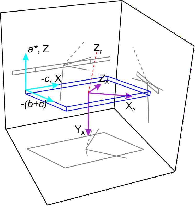
Figure 6: (color online) Orientation of the cartesian basis used for calculations with respect to the crystal axes and orientations of anisotropy and $g$-tensor axes found from the modeling.

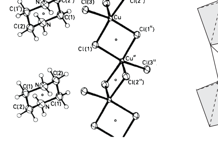
Figure 7: Left: Fragment of the PHCC crystallographic structure (from Ref.structure, ). Vertical direction corresponds to the crystallographic $\mathbf{c}$ axis. Right: Orientations of the distorted chlorine pyramids. Positions of copper and apical chlorine ions are shown. Visible bases of the pyramids are shadowed in grey.

Different models are used for the description of the low energy dynamics of a spin gap magnet in magnetic field. A fermionic field-theory model was proposed for 1D systems by Tsvelik tsvelik . Alternatively, a bosonic field-theory model was proposed by Affleck Affleck and later independently developed as a macroscopic model by Farutin farmar . Particular systems can be treated by microscopic approaches Kolezhuk . However, only close to the critical field the differences of all these models become important. Since we can not observe singlet-triplet transitions on PHCC, we can not look for these fine differences and can not reliably judge on the applicability of different models from the ESR data alone. On the other hand, since our data correspond to the low-field limit (the critical field is around 8 T, while all X-band resonance modes are below 1 T and most of the higher frquency data are below 4 T) we can apply a perturbative approach for the description of the observed ESR data. It will yield the values of zero-field splitting of the energy levels and the orientations of all relevant anisotropy axes which can be used, if necessary, to obtain parameters of other models.

This approach considers triplet excitations for a non-interacting $S=1$ particle moving in a stationary effective crystal field. The effective spin Hamiltonian for this particle is:

$$\widehat{\cal{H}}=\Delta+\mathbf{H}\cdot\widetilde{g}\cdot\widehat{\mathbf{S}}+D\widehat{S}_{Z_{A}}{}^{2}+E(\widehat{S}_{X_{A}}{}^{2}-\widehat{S}_{Y_{A}}{}^{2})$$ (1)

where $\Delta$ is an energy gap, $\widetilde{g}$ is a $g$-tensor, $D$ and $E$ are the effective anisotropy parameters and $\mathbf{X}_{A}$, $\mathbf{Y}_{A}$, $\mathbf{Z}_{A}$ are the anisotropy axes. Due to the triclinic crystal symmetry the orientation of the anisotropy axes $\mathbf{X}_{A}$, $\mathbf{Y}_{A}$, $\mathbf{Z}_{A}$ is arbitrary with respect to the crystal. Moreover, the $g$-tensor axes $\mathbf{X}_{g}$, $\mathbf{Y}_{g}$, $\mathbf{Z}_{g}$ are also arbitrary with respect both to the crystal and to the anisotropy axes. We neglect here the $\mathbf{k}$-dependence of the Hamiltonian parameters $D$ and $E$, since at low temperatures only the bottom of the spectrum is populated, while at high temperatures the exchange narrowing cancels out the effects of these terms.

The perturbative model can be solved for eigenenergies for any given magnetic field. The differences of the eigenenergies will correspond to the resonance frequencies which can then be compared with the experiment. We used a standard least-squares routine to minimize the model deviation from the experimental data.

Angular dependences of the X-band resonance fields at 3 K and 25 K were used for the determination of the Hamiltonian parameters. Additionally, the values of the $g$-factor and the low-temperature splittings measured in the high-frequency experiments with well-defined sample orientation were used as anchors to correct for the angle shifts due to the sample mounting. The basis $\mathbf{X}$, $\mathbf{Y}$, $\mathbf{Z}$ with $\mathbf{Z}||\mathbf{a}^{*}$ and $\mathbf{X}||(-\mathbf{c})$ was selected to describe the orientation of the $g$-tensor and the anisotropy axes with respect to the crystal (Figure 6).

This problem has 14 parameters: the anisotropy constants $D$ and $E$, the Euler angles of the anisotropy axes $\alpha_{A}$, $\beta_{A}$ and $\gamma_{A}$, three main values of the $g$-tensor, the Euler angles of the $g$-tensor axes, and, finally, three uncontrolled shift angles $\epsilon_{1,2,3}$ in the X-band rotation experiments. It turned out, that this general fit yields two of the $g$-tensor components very close to each other (best fit $g$-factor values 2.272, 2.062 and 2.039). Consequently, the fit became unstable and could not well distinguish the orientations of the $g$-tensor differing by rotation around high-$g$-value axis. Thus, we reduced the number of model parameters to 12 by assuming an axial $g$-tensor that can be described by two main values and by two polar angles of the $g$-tensor axis. The stability of the best fit solution was confirmed by running numerous fitting procedures with randomly varied initial approximations of the model parameters.

Table 1: Best fit parameters in the perturbative model.

anisotropy	D, MHz	$-7900\pm 280$
constants	E, MHz	$-1340\pm 190$
$g$-tensor	$g_{||}$	$2.280\pm 0.015$
main values	$g_{\perp}$	$2.048\pm 0.007$
Euler angles	$\alpha_{A}$	$(-43.5\pm 1.8)^{\circ}$
of anisotropy	$\beta_{A}$	$(-105.6\pm 1.5)^{\circ}$
axes	$\gamma_{A}$	$(-12.5\pm 7)^{\circ}$
Polar angles of	$\Theta_{g}$	$(105\pm 3)^{\circ}$
$g$-tensor axes	$\phi_{g}$	$(54.9\pm 1.5)^{\circ}$
shift	$\epsilon_{1}$	$(-10.9\pm 3.5)^{\circ}$
angles	$\epsilon_{2}$	$(41\pm 2.5)^{\circ}$
	$\epsilon_{3}$	$(-4.0\pm 3.5)^{\circ}$

The best fit parameters are shown in the Table 1 and the corresponding frequency-field and angular dependences are shown in the Figures 3, 4. The orientation of the anisotropy axes and $g$-tensor axis are illustrated at the Figure 6. The sign of anisotropy constants can be unambiguously determined by comparing low-temperature intensities of the split absorption components in different orientations (Figure 2): a more intense absorption corresponds to the transition from the lower sublevel.

The found axiality of the $g$-tensor can be explained by the details of the microscopic structure of PHCC.structure Each copper ion is surrounded by five chlorine ions, forming a distorted square-based pyramid (Figure 7). The main axis of this pyramid is the same for all copper ions (differently oriented pyramids are connected by inversion). The direction of the vector linking the copper to the apical chlorine (position Cl(2) in the denominations of Ref.structure, ) is very close to the found direction of the $g$-tensor axis: its polar angles in the chosen reference frame are $\Theta_{Cu-Cl}=111^{\circ}$ and $\phi_{Cu-Cl}=57^{\circ}$.

IV.3 Anisotropic corrections and critical field.

Table 2: Comparison of the measured parameters of the excitation spectrum and calculated parameters in different models. Values of $g$-factor are given for reference as calculated for particular orientations using a best fit perturbative model. For the precision of the model estimations see footnote .

	Experiment	$g$-factor	pertur-	macro-
		anisotropy	bative	scopic
		only	model	model
Zero-field			233.6	234.0
energies,	247	235.6	236.2	236.6
GHz			242.8	243.2
$\mu_{0}H_{c}$,T:
$\mathbf{H}\perp(-1,1,0)$	$7.90\pm 0.07$	7.71	7.74	7.70
($g=2.183$)
$\mathbf{H}||\mathbf{a}^{*}$	$8.29\pm 0.05$
($g=2.064$)	$8.03\pm 0.07$	8.15	8.27	8.19
$\mathbf{H}||\mathbf{b}$	$7.47\pm 0.01$	7.47	7.47	7.47
($g=2.253$)	$7.58\pm 0.03$
	$7.40\pm 0.08$
$\mathbf{H}||\mathbf{c}$	$7.6\pm 0.2$	7.93	7.96	7.89
($g=2.122$)

Our specific heat measurement and earlier measurements of other authors demonstrate the anisotropy of the critical field of about 1 T (see Table 2). Additionally, neutron scattering experiments broholm-njp2007 ; stone-prl96 have determined the orientation of the order parameter above the critical field for $\mathbf{H}||\mathbf{b}$: the order parameter was found to lie within $(7\pm 4)^{\circ}$ of the $(ac)$ plane with an in-plane component within $(6\pm 4)^{\circ}$ of the $a$-axis. Both of these effects are determined by the anisotropic interactions in the spin system and thus provide an independent check for the anisotropy parameters found above.

The critical field depends strongly on temperature: its values at 65mK and at 2.8K differ by $\approx 2$T broholm-njp2007 . Thus, it is necessary to ascertain whether the anisotropy parameters determined at 3.0K can be used in the analysis of the low temperature data or not.

The temperature dependence of the critical field originates from the renormalization of the energy spectrum due to the repulsive interaction of triplet excitations. This renormalization depends on the triplet population numbers and therefore affects strongly the energy spectrum in the vicinity of the critical field, where the energy gap is small. Our ESR measurements, on the contrary, were performed in small fields where the energy gap value is still high and the triplet population numbers are small even at 3.0K. This is confirmed by the experimental observation that the observed splitting of the resonance absorption does not change significantly at further cooling below 3K. Therefore, the effect of triplet repulsion does not affect the values of anisotropy parameters found in the previous subsection and these values can be used for the analysis of the low temperature data for the critical field anisotropy and order parameter orientation.

In the model calculations of this subsection we will use $g$-factor values and (when necessary) zero-field splittings as determined in our ESR experiments. Since the gap value $\Delta$ can not be determined with the similar precision, we will tune it to obtain correct value of the critical field in the chosen orientation. We choose the value of the field at which the antiferromagnetic Bragg reflection appears broholm-njp2007 at $\mathbf{H}||\mathbf{b}$ ($\mu_{0}H_{c}=7.47\pm 0.01$T) as the most reliable anchor for this purpose.

First, there is a simplest model, suggested in Ref. broholm-njp2007, , that treats the anisotropy of the critical field as originating from the $g$-factor anisotropy only. This model was backed by the observation that the ratios of the critical field to the saturation field were found to be the same in different orientations. The values of the $g$-factor in the particular orientations of the magnetic field calculated from our model are given in Table 2. One can see that the highest critical field is indeed observed in the direction with the smallest $g$-value ($\mathbf{H}||\mathbf{a}^{*}$). The critical field in the arbitrary orientation can be expressed via the $g$-factor value as $H_{c}=(g(\mathbf{H}||\mathbf{b})H_{c}(\mathbf{H}||\mathbf{b}))/g$. The calculated values are in reasonable agreement with the experiment (see Table 2).

However, this simple model is not exact, since we observe zero-field splitting of energy levels. The effect of zero-field splitting on the anisotropy of the critical field can be roughly estimated from the value of the main anisotropy constant as $\mu_{0}\Delta H_{A}\sim hD/(g\mu_{B})\approx 0.3$T. This has to be compared with the effects of the $g$-tensor anisotropy: $\mu_{0}\Delta H_{g}\sim(\Delta g/g)\mu_{0}H_{c}\approx 0.9$T. These values are similar and, especially since the axes of anisotropy and the axes of $g$-tensor do not coincide, it is not possible to neglect a priori one of the effects for an arbitrary field direction.

As a second test model, we extrapolate the results of the perturbative model up to the critical field. This extrapolation can be justified only for one-dimensional systemszaliznyak . However, this model can be considered as a simple approximation taking into account both the effects of $g$-tensor anisotropy and zero-field splitting of triplet sublevels. The results of this extrapolation are also collected in Table 2.

Finally, the problem of the triplet level field dependence can be treated more strictly within the frameworks of a macroscopic (bosonic) approachfarmar ; Affleck . This model treats the excitations of a spin-gap magnet as oscillations of the vector field $\boldsymbol{\eta}$ with the Lagrangian

$${\cal{L}}=\frac{1}{2}\left(\dot{\boldsymbol{\eta}}+\gamma[\boldsymbol{\eta}\times\mathbf{H}]\right)^{2}-\frac{1}{2}A\boldsymbol{\eta}^{2}+{\cal{L}}_{rel}$$ (2)

where $A$ is the exchange constant describing the energy gap, $\gamma$ is the gyromagnetic ratio and ${\cal{L}}_{rel}$ is a term containing anisotropic relativistic corrections. The leading corrections terms at low fields are the effective anisotropy terms, responsible for the zero field splitting, which can be written in the reference frame of anisotropy axes $(X_{A},Y_{A},Z_{A})$:

$${\cal{L}}_{rel1}=\frac{1}{2}b_{1}(\eta_{X_{A}}^{2}+\eta_{Y_{A}}^{2}-2\eta_{Z_{A}}^{2})+\frac{1}{2}b_{2}(\eta_{X_{A}}^{2}-\eta_{Y_{A}}^{2})$$ (3)

where $b_{1,2}$ are the effective anisotropy constants. These terms allow to describe the zero field splitting, see e.g. Ref.glazkov-ntenp, .

To describe additional field effects we have to include here next order terms. The low symmetry of the crystal allows numerous relativistic and exchange-relativistic invariants such as $\dot{\eta}_{\alpha}\dot{\eta}_{\beta}$, $[\boldsymbol{\eta}\times\dot{\boldsymbol{\eta}}]_{\alpha}H_{\beta}$, $(\mathbf{H}\boldsymbol{\eta})H_{\alpha}\eta_{\beta}$, $H^{2}\eta_{\alpha}\eta_{\beta}$, $\boldsymbol{\eta}^{2}H_{\alpha}H_{\beta}$ etc. I.e., in general we have to consider a veritable zoo of possible terms which overburdens the problem beyond any hope to produce a compact solution.

To simplify this problem we will assume that the main field effects arise from a single-ion $g$-tensor anisotropy. Thus, due to an almost tetragonal local symmetry, these effects can be considered as having an axial symmetry in the $g$-tensor reference frame. Additionally, we will require that for the model test case of $b_{1}=b_{2}=0$ these terms should provide linear E(H) dependences for all three modes, which is natural for the microscopic model with anisotropic single-ion $g$-tensor only.

This leads to the following invariants combination:

$${\cal{L}}_{rel2}=\xi(\gamma^{2}H_{Z_{g}}^{2}\boldsymbol{\eta}^{2}-\gamma^{2}(\mathbf{H}\boldsymbol{\eta})H_{Z_{g}}\eta_{Z_{g}}+\gamma H_{Z_{g}}[\dot{\boldsymbol{\eta}}\times\boldsymbol{\eta}]_{Z_{g}})$$ (4)

where the parameter $\xi=(g_{||}/g_{\perp}-1)$ reflects the $g$-factor anisotropy. Up to higher order corrections, equation (4) is equal to the replacement of the problem with an anisotropic $g$-tensor $\tilde{g}$ and a certain real field direction $\mathbf{H}$ by the formally equivalent problem with the isotropic $g$-factor $g_{0}$ and a transformed ”effective” field $\mathbf{H}_{eff}=(1/g_{0})(\tilde{g}\mathbf{H})$. Three terms in Eqn.(4) are responsible for different effects and none can be omitted.

The dynamics equations can be obtained from the final Lagrangian ${\cal{L}}+{\cal{L}}_{rel1}+{\cal{L}}_{rel2}$ using a standard variational technique with special attention to the frames of reference (see Appendix). The solution of these equations yields the field dependences of the energy levels, whose differences would yield transition frequencies. The parameters of the macroscopic model can be directly expressed via perturbative model parameters with only one adjustable parameter $\Delta$:

$$A = 4\pi^{2}(\Delta^{2}+(\Delta+D+E)^{2}+(\Delta+D-E)^{2})/3$$

$$b_{1} = 4\pi^{2}(2\Delta^{2}-(\Delta+D+E)^{2}-(\Delta+D-E)^{2})/6$$

$$b_{2} = 4\pi^{2}((\Delta+D+E)^{2}-(\Delta+D-E)^{2})/2$$

$$\gamma = 2\pi(g_{\perp}/2.0)\gamma_{0}$$

$$\xi = (g_{||}/g_{\perp}-1)$$

here $\gamma_{0}=2.80$GHz/kOe is a free electron gyromagnetic ratio. The factors of $4\pi^{2}$ or $2\pi$ appears here since the dynamics equations (13) are written for angular frequency $\omega$, while the parameters of the perturbative model were expressed in the ordinary frequency units.

The parameters values corresponding to $\mu_{0}H_{c}(\mathbf{H}||\mathbf{b})=7.47$T are: $A=2.236\cdot 10^{24}$ 1/sec², $b_{1}=4.972\cdot 10^{22}$ 1/sec², $b_{2}=-2.490\cdot 10^{22}$ 1/sec², $\gamma/(2\pi)=2.867$GHz/kOe, $\xi=0.1133$.

We have found that the model curves fits our data perfectly and are undistinguishable from the perturbative curves at low fields. The predicted values of critical fields are also gathered in the Table 2.

The macroscopic model allows a straightforward analysis of the order parameter orientation above the critical field. We have to add to the final Lagrangian fourth order exchange term $-B\boldsymbol{\eta}^{4}$ which will determine the magnitude of the order parameter at $H>H_{c}$.farmar However, as long as all anisotropic terms are of the same order in $\boldsymbol{\eta}$, the orientation of the order parameter does not depend on its amplitude and, consequently, does not depend on the value of the exchange constant $B$. Thus, for the sake of determining the order parameter orientation only, the $B$ constant can be simply thought of as a mathematical meaning to exclude the divergence of the order parameter above $H_{c}$. Using the model parameters described above we have found that the polar angles of order parameter at $\mathbf{H}||\mathbf{b}$ are $\Theta_{O.P.}=34^{\circ}$ and $\phi_{O.P.}=-20^{\circ}$. This corresponds to an angle of 16^∘ with the $(ac)$-plane and to an angle of 28^∘ to the $a$-axis. The in-plane component of the calculated order parameter forms an angle of $23^{\circ}$ with the $a$-axis. Although there is a qualitative agreement, the calculated values differ from those found in the experiment broholm-njp2007 ; stone-prl96 .

All of the models provide a reasonable qualitative agreement with the experiment. The macroscopic model seems to be physically the most justified, since it describes correctly the zero-field structure of energy levels and can be applied up to the critical field and above. Quantitative disagreements with the experiment can be caused by some neglected factors: the slight change of anisotropy constants at cooling below 3K or the effects of additional anisotropic contributions above $H_{c}$.

V Conclusions.

A detailed investigation of the low-energy spin dynamics in the spin-gap magnet PHCC revealed the presence of anisotropic interactions causing a splitting of the triplet sublevels and leading to a $g$-tensor anisotropy. The effects of these interactions were described quantitatively within a perturbative approach in small fields. The parameters of anisotropy comprising the main $g$-tensor values, the zero-field splitting of sublevels and the orientations of corresponding axes with respect to the crystal were found. Additionally, an application of the macroscopic (bosonic) model to the case of a spin gap magnet with a relevant $g$-factor anisotropy was developed.

Appendix A Dynamics equation for macroscopic (bosonic) model with axial $g$-tensor below $H_{c}$.

The complete Lagrangian of the problem can be obtained from Eqns.(2),(3),(4):

$$\cal{L} = \frac{1}{2}(\dot{\boldsymbol{\eta}}+\gamma[\boldsymbol{\eta}\times\mathbf{H}])^{2}-\frac{1}{2}A\boldsymbol{\eta}^{2}+$$ (5)

$$+ \frac{1}{2}b_{1}(\eta_{X_{A}}^{2}+\eta_{Y_{A}}^{2}-2\eta_{Z_{A}}^{2})+\frac{1}{2}b_{2}(\eta_{X_{A}}^{2}-\eta_{Y_{A}}^{2})+$$

$$+ \xi\gamma^{2}H_{Z_{g}}^{2}\boldsymbol{\eta}^{2}-\xi\gamma^{2}(\mathbf{H}\boldsymbol{\eta})H_{Z_{g}}\eta_{Z_{g}}+$$

$$+ \xi\gamma H_{Z_{g}}[\dot{\boldsymbol{\eta}}\times\boldsymbol{\eta}]_{Z_{g}}$$

The same coefficient $\xi$ in the last three terms is a consequence of the microscopic model that assumes a single-ion $g$-tensor anisotropy with an axial $g$-tensor. Due to the low symmetry of the crystal, terms responsible for the effective anisotropy ($b_{1}$ and $b_{2}$ terms) and for the $g$-factor anisotropy ($\xi$-terms) are written in different cartesian bases. When varying the Lagrangian over $\boldsymbol{\eta}$ these terms have to be recalculated to the same basis. We used the anisotropy axes basis for the derivation of the dynamics equation. The resulting dynamics equation on $\boldsymbol{\eta}$ is:

$$\ddot{\boldsymbol{\eta}}+2\gamma[\dot{\boldsymbol{\eta}}\times\mathbf{H}]-\gamma^{2}H^{2}\boldsymbol{\eta}+\gamma^{2}\mathbf{H}(\boldsymbol{\eta}\cdot\mathbf{H})+A\boldsymbol{\eta}-$$

$$- b_{1}\left(\begin{array}[]{c}\eta_{X_{A}}\\ \eta_{Y_{A}}\\ -2\eta_{Z_{A}}\\ \end{array}\right)-b_{2}\left(\begin{array}[]{c}\eta_{X_{A}}\\ -\eta_{Y_{A}}\\ 0\\ \end{array}\right)-\xi\gamma^{2}(\mathbf{H}\mathbf{Z}_{g})^{2}\boldsymbol{\eta}+$$

$$+ \xi\gamma^{2}(\mathbf{H}\mathbf{Z}_{g})((\boldsymbol{\eta}\mathbf{Z}_{g})\mathbf{H}+(\boldsymbol{\eta}\mathbf{H})\mathbf{Z}_{g})-$$

$$- 2\xi\gamma(\mathbf{H}\mathbf{Z}_{g})[\mathbf{Z}_{g}\times\boldsymbol{\eta}]=0.$$ (13)

This equation yields a secular equation for the precession circular frequencies $\omega_{1,2,3}$ that describes the field dependence of the energy levels. The latter is a cubic equation for $\omega^{2}$ and can be solved for any field direction.

References

- (1) M.B. Stone, C. Broholm, D.H. Reich, P. Schiffer, O. Tchernyshyov, P. Vorderwisch and N.Harrison, New Journal of Physics 9, 31 (2007)
- (2) M.B. Stone, I. Zaliznyak, D.H.Reich and C.Broholm Physical Review B 64, 144405 (2001)
- (3) M.B. Stone, I.A. Zaliznyak, Tao Hong, C.L. Broholm and D.H.Reich, Nature 440,187 (2006)
- (4) L.P. Battaglia, A.B. Corradi, U. Geiser, R. Willett, A. Motori, F. Sandrolini, L. Antolini, T. Manfredini, L. Menaube and G. Pellacani J. Chem. Soc. Dalton. Trans. 2 265 (1988)
- (5) Ian Affleck, Physical Review B 46, 9002 (1992)
- (6) A.M. Farutin and V.I. Marchenko, Zh.Eksp.Teor.Fiz. 131 860 (2007) (JETP 104 751 (2007))
- (7) V.N.Glazkov, A.I. Smirnov, H. Tanaka and A. Oosawa. Physical Review B, 69 184410 (2004).
- (8) V.N. Glazkov, A.I. Smirnov, A. Zheludev, and B.C. Sales, Physical Review B 82, 184406 (2010)
- (9) A. Abragam, B. Bleaney, Electron paramagnetic resonance of transition ions.
- (10) A.M. Tsvelik, Physical Review B 42, 10499 (1990)
- (11) A.K. Kolezhuk, V.N. Glazkov, H. Tanaka, and A. Oosawa Physical Review B 70, 020403 (2004)
- (12) M.B. Stone, C. Broholm, D.H. Reich, O. Tchernyshyov, P. Vorderwisch and N. Harrison Physical Review Letters 96, 257203 (2006)
- (13) L.-P. Regnault, I.A. Zaliznyak and S.V. Meshkov J.Phys.:Condens.Matter 5 L677 (1993)