Salt-and-Pepper Noise Removal Based on Sparse Signal Processing

Abstract

In this paper, we propose a new method for Salt-and-Pepper noise removal from images. Whereas most of the existing methods are based on Ordered Statistics filters, our method is based on the growing theory of Sparse Signal Processing. In other words, we convert the problem of denoising into a sparse signal reconstruction problem which can be dealt with the corresponding techniques. As a result, the output image of our method is preserved from the undesirable opacity which is a disadvantage of most of the other methods. We also introduce an efficient reconstruction algorithm which will be used in our method. Simulation results indicate that our method outperforms the other best-known methods both in term of PSNR and visual criterion. Furthormore, our method can be easily used for reconstruction of missing samples in erasure channels.

Index Terms—Sparse Signal Reconstruction, Compressed Sensing, Iterative Method with Adaptive Thresholding, Salt-and-Pepper Noise Removal, Dual-Tree Complex Wavelet.

I Introduction

During the last years, sparse signal processing has recieved a growing attention. In fact, many natural phenomena result in signals which are sparse in some domain, i.e., most of their components are zero. Generally, let $x$ be an $n\times 1$ sparse signal i.e., it has only $k$ non-zero elements where $k\ll n$. As an extension to Niquist/Shanon sampling theorem, one can think of unique reconstruction of $x$ from only 2$k$ equations. In other words, $x$ can be uniquely determined by the knowledge of location and amplitude of its nonzero elements (which are totally 2$k$ unknowns). As an example, let $x$ be a $k$-sparse signal in time domain and $\Phi$ be an $m\times n$ matrix ($k\textless m\textless n$) which may be achieved by selecting m rows of a DFT matrix. Considering $y$ as

$$y=\Phi\mathbf{x}$$ (1)

it contains m samples of signal $x$ in the frequency domain. Sparse signal processing is concerned with the conditions and methods of determining $x$ out of $\Phi$ and $y$. Generally, $\Phi$ can be any arbitrary transformation submatrix and sparsity of $x$ can be in other domains such as frequency, space and etc.

In a close relationship with the Compressed Sensing (CS) theory [1, 2, 3], signal $x$ is the answer of the following non-convex optimization:

$$min||x||_{0}\leavevmode\nobreak\ \leavevmode\nobreak\ \leavevmode\nobreak\ \leavevmode\nobreak\ \leavevmode\nobreak\ s.t.\leavevmode\nobreak\ \leavevmode\nobreak\ \leavevmode\nobreak\ \leavevmode\nobreak\ \leavevmode\nobreak\ \Phi\mathbf{x}=y.$$ (2)

Since the above problem is difficult to handle, the $\ell_{0}$ norm is usually replaced by $\ell_{1}$ norm which under some conditions yields the same result. There are several approaches to solve the $\ell_{1}$-minimization problem such as Spectral Projected Gradient for L1 minimization (SPGL1) [4], Least Absolute Shrinkage and Selection Operator (LASSO) [5]. Due to the high complexity of these methods, they are not practically used and most attentions are focused on designing fast and stable reconstruction algorithms. These algorithms - known as Greedy algorithms - provide the best estimation of $x$ by processing on $\Phi$ and $y$ in (1). The best-known greedy algorithms in the literature are Orthogonal Matching Pursuit (OMP) [6], Compressive Sampling Matching Pursuit (CoSaMP) [7], and Iterative Hard Thresholding (IHT) [8].

Consequently, by using sparse signal processing techniques, a sparse signal can be reconstructed from a number of its samples in another domain. This fact is the basic idea of using sparse processing in different applications. Unfortunately, most of the mentioned reconstruction algorithms are designed for 1-D signals. However, reconstruction of sparse signals can be addressed for 2-D signals as well, but here the problem cannot be expressed as in (1).

In this paper, we use sparse processing techniques to remove Salt-and-Pepper noise from images, thus we will face the problem of reconstruction of a 2-D signal using its samples in another basis. Since the existing algorithms are not always suitable for 2-D problems, we have employed a novel algorithm capable of reconstruction of 2-D signals.

Images often get corrupted by impulsive noise during the acquisition or transmission. Salt-and-Pepper noise is a usual kind of impulsive noise which changes the value of a percentage of pixels into maximum or minimum allowed value. Removal of Salt-and-Pepper noise is an important pre-processing step because it can influence the subsequent phases in image processing such as segmentation, edge detection and recognition.

Several methods have been proposed to remove Salt-and-Pepper noise. Of all the filters reported in image restoration domain, the Ordered Statistics (OS) filters such as median filter and its variants are the most prominent due to their computetional efficiency and simplicity. Amoung these methods are Adaptive Median Filter (AMF) [9] which with adaptive window size tries to grasp more detail information for removing the noisy pixels. In [10], Progressive Switching Median Filter (PSMF) is proposed for highly corrupted environments. A Detail-Preserving Median Filter (DPMF) is proposed in [11] which removes Salt-and-Pepper noise while keeping the fine details of the image. Some of the other best existing methods are Decision-Based Algorithm (DBA) [12] which replaces the corrupted pixels by the median of the neighbouring pixel value, Edge-Preserving Algorithm (EPA) [13] which adopts a directional correlation-dependent filtering technique, Switching-based Adaptive Weighted Mean filter (SAWM) [14] which replaces each noisy pixel with the weighted mean of its noise-free neighbours, and Adaptive Iterative Mean filter (AIM) [15] which is adaptive in term of the number of iteration for each noisy pixel. In [16], Recursive Detection-Estimation (RDE) method is introduced which iteratively remove the noise. In this paper, we will propose a new method based on sparse processing and compare it with the above techniques.

This paper is organized as follows: In Section II, we introduce the reconstruction algorithm used in our method. In Section III, we will address the problem of Salt-and-Pepper noise removal and provide basics of our method. Section IV contains in details the discription of our method, and simulation results are discussed in Section V. Finally, we conclude the paper in Section VI with future work.

II Proposed Reconstruction Algorithm

As mentioned in Section I, most of the existing reconstruction algorithms are designed to estimate 1-D sparse signals from their samples in another domain. However, for 2-D signals, these algorithms are incapable of performing this task efficiently. In fact, they need to convert 2-D problems into 1-D problems which makes it computationally complex. In the following, we introduce a newly designed reconstruction algorithm which can be directly used for problems in higher dimensions.

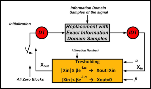
Figure 1: Block Diagram representation of IMAT.

The reconstruction algorithm used in our method is called Iterative Method with Adaptive Thresholding (IMAT) [17, 18] which is depicted in Fig. 1. In this figure, the DT and IDT blocks represent a Discrete Transform and Inverse of that transform, respectively. Let $x$ be a sparse signal in an arbitrary domain ($B1$) which we have some of its samples in another domain ($B2$). To reconstruct $x$ using the IMAT, the DT block here is the operator which transforms signals from B1 to B2.

To initialize in the IMAT method, the signal is estimated as an all-zero signal. Next, the estimated signal is converted into the information domain (B2), which replaces the specified samples. Then, after transforming the signal into the sparsity domain ($B1$), it is necessary to make the signal sparse. This task is performed by a thresholding block which converts all the components below a specific threshold to zero. The algorithm goes on iteratively. As the algorithm proceedes, the estimated signal is more similar to the original one; Thus, it is necessary to reduce the threshold as the iteration number increases. In IMAT, the threshold decays exponentionally as in Fig. 1. The steps of the IMAT method are also listed in Table I.

The important virtue of this method among the MP methods is application to 2-D signals. We will utilize this algorithm in our denoising method.

Table I: IMAT Reconstruction Algorithm.

1) Use an all-zero vector as the initial value for the sparse domain signal. ( iteration 0)

2) Convert the current estimate of the signal in the sparse domain into the information domain using the known Discrete Transform.

3) Replace the inexact values of the estimated signal with the exact, but still noisy, samples in the information domain.

4) Use IDT to return to the sparse domain.

5) Hard-threshold the signal with an adaptive exponential threshold as mentioned in Fig. 1.

6) Continue steps 2-5 until the stop criterion. (e.g. maximum iteration number or minimum error between estimations) has been met.

III Problem Definition

In this section, we will introduce a model of Salt-and-Pepper noise and provide the details of our denoising method. As mentioned previously, most of the existing denoising methods in the literature are based on Ordered Statistics filters in which undesired opacity is inevitable. Our proposed method is based on sparse processing techniques which results in an vivid image.

Let $Y$ be an $n\times n$ matrix representing the noise-free image. The image corrupted by Salt-and-Pepper noise can be modelled as:

$$Z=Y+N$$ (3)

where $Z$ indicates the noisy image and $N$ is the noise matrix which changes the value of a percentage of the image pixels into maximum or minimum allowed value. The problem here is to find $Y$ from $Z$.

As a fact, image signals can be represented as sparse 2-D signals for some well-known transforms such as $Discrete$ $Cosine$ $Transform$ (DCT) and various kinds of $wavelets$. In other words, when DCT or wavelet transform is applied on an image, a sparse matrix is resulted, i.e., a matrix that most of its entries are nearly zero. Therefore, one can think of a sparse representation of $Y$ (the noise-free image) in some domain. In this paper, we will consider a newly designed wavelet transform called as $Dual$-$Tree$ $Complex$ ($DTC$) wavelet [19, 20] which has been widely used in image and video processing applications recently. The main virtue of this type of wavelet is that image signals have a more sparse representation in this domain in comparison to that of Daubechies wavelet or DCT. To be more clear, there exist a sparse matrix like $X$ such that:

$$X=wavelet(Y).$$ (4)

Obviously, if we can obtain $X$, the original image can be achieved by applying the inverse wavelet transform on $X$. The method is explained in details in the following section.

IV Proposed Denoising Method

As mentioned in the previous section, the problem of image denoising is equivalent to a sparse signal signal reconstruction problem. In other words, our approach is to estimate a 2-D sparse signal ($X$) using sparse signal processing. To obtain the noise-free image ($Y$) out of the noisy image ($Z$), our approach is to determine the DTC wavelet transform of the image (i.e., $X$). As metioned previously, $X$ is a 2-D sparse signal (in the wavelet domain). Consequently, by using sparse signal processing techniques, $X$ can be reconstructed from a number of its samples in another domain. As a fact, the pixels of $Y$ are all the samples of $X$ in the space domain. On the other hand, the noise-free pixels of the noisy image (i.e., $Z$) can be identified using noise detection algorithms. According to (3), the noise-free entries of $Z$ are amoung the entries of $Y$ (because $N$ is zero in these positions).

Consequently, finding the noise-free pixels of $Z$, we have obtained a number of $Y$ pixels which are in fact the samples of $X$ in the space domain. Thus, $X$ can be determined via sparse signal reconstruction techniques using these samples.

To find the noise-free pixels of $Z$ in our method, we simply find those pixels with the value unequal to the maximum or minimum allowed value. Of course, some of the noise-free pixels may be regarded as noisy pixels in this procedure, but it does not affect the performance of our method significantly. We use the IMAT method to reconstruct $X$ out of its samples and finally the noise-free image is obtained by applying the inverse wavelet transform on $X$.

V Simulation Results

Table II: $PSNR$ of different denoising methods for image Lena (scenario 1).

Noise Ratio	EPA	DBA	SAWM	AIM	AMF	PSMF	DPMF	our Method
10 %	42.5537	41.0363	43.2251	43.3576	38.1756	35.7154	35.7671	44.5412
20 %	38.8488	37.0136	39.7376	39.6616	35.9044	31.5767	36.2589	41.2143
30 %	36.6843	34.0029	37.3747	37.3064	33.8722	27.9894	35.7035	39.2923
40 %	34.3982	31.4783	35.4690	35.5484	31.9158	24.6979	34.2164	37.5230
50 %	33.1593	29.4906	33.8417	34.0615	30.3444	21.5247	32.9932	35.7547
60 %	31.4457	27.3464	32.3867	32.8013	28.5645	23.2599	31.4285	34.2997
70 %	29.7428	25.1534	30.6842	31.4891	26.7704	18.9913	29.7656	32.4291

In this section, we implement our proposed method for Salt-and-Pepper noise removal and compare it against the other well-known algorithms in the literature. Generally, there are two scenarios under which an image can be corrupted by Salt-and-Pepper noise. In the first one, an existing image may be corrupted by Salt-and-Pepper noise due to physical phenomena over time. In such a scenario, the image which is corrupted by the noise is the original image without any pre-adaptation. This scenario is widely considered in the literature. However, we consider a second scenario as well. As mentioned in section III, images are not really sparse in the DCT or wavelet transforms. In fact, most of their coefficients are very close to zero but not exactly zero. In comunication systems, these nearly zero coefficients are set to zero in the transmitter, and then sparsed version of the original image is transmitted. As a result, the noisy version of the sparsed image (not the original one) is recieved. Hence, in the second scenario, the problem is denoising of a sparsed image.

For the first scenario, The simulations are performed for different standard images and for different noise densities. In Fig. 2, the performance of our method is tested for Lena (80% Salt-and-Pepper noise) and Baboon (70% Salt-and-Pepper noise).

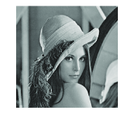
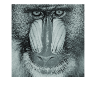
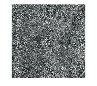
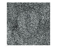
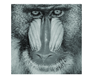
Figure 2: Simulation results of proposed method in scenario 1, (a) Lena original image, (b) Baboon original image, (c) 80% Noisy image, (d) 70% Noisy image, (e) Reconstructed image, (f) Reconstructed image.

In Table II, we have compared the proposed method against other methods for the image Lena with different noise densities (10% to 70%). It depicts that our method outperforms the other ones in all cases. The criterion here is Pick Signal to Noise Ratio (PSNR).

In addition to the PSNR criterion, our method seems to be better than the other methods in visual criterion. Figure 3 contains the output images of our method and three of the other best-known methods in 60% Salt-and-Pepper noise of the image Boat. As depicted in this figure, our method preserves the image from opacity while all the other methods suffer from some kind of distortion. This distortion is more recognizable along the edges. According to the socond scenario, we compared our method with other methods to denoise a sparsed image. Table III represents the comparison results for our method and three of the best-known methods in PSNR. Here, we have assumed that 80% of image samples in the wavelet domain are set to zero at the transmitter (i.e., the image is 20% sparsified). As depicted in Table III, sparsifing the image in tha transmitter improves the performance of our method.

Table III: PSNR for different methods for sparsed Lena (scenario 2).

Noise Ratio	EPA	SAWM	AIM	our Met.
10 %	39.5301	39.7418	44.7401	49.5318
20 %	37.4529	37.9983	40.8498	45.6537
30 %	36.0217	36.4273	38.3235	42.6723
40 %	34.2842	35.0963	36.4584	40.1646
50 %	32.8376	33.8025	34.9292	37.8776
60 %	31.4505	32.3142	33.5804	35.8904
70 %	29.9763	30.7672	32.0970	33.5349

It is worth mentioning that our proposed method can be directly used to reconstruct the images which some of their samples are lost due to an erasure channel.

In the IMAT method, we have selected $\alpha$ (defined in Fig. 1) as 0.1, and $\beta$ is set to be a little greater than the maximum absolute value of the image signal.

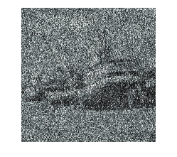
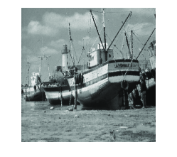
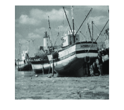
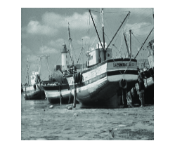
Figure 3: Simulation results for Boat image in scenario 1, (a) Original image, (b) 60% Noisy image, (c) EPA, (d) SAWM, (e) AIM, (f) Proposed method.

VI Conclusion

In this paper, we proposed a new nonlinear method for removing Salt-and-Pepper noise from images. Our method is based on sparse signal processing. In fact, we convert the denoising proplem into a sparse reconstruction problem. In addition, since most of the existing reconstruction algorithms are incapable of being used in our method, we have introduced a novel reconstruction algorithm as well.

As a result of this approach, our method preserves the image from the distortion which is occuring in most of the existing denoising methods based on spatial OS filters.

Simulation results confirms the prominence of the proposed method against the best-known existing methods. In the future, we will use the idea of our method for removing block noises from images.

References

- [1] D. Donoho, “Compressed sensing,” IEEE Trans. Inf. Theory, vol. 52, no. 4, pp. 1289–1306, April 2006.
- [2] E. Candes and J. Romberg, “Sparsity and incoherence in compressive sampling,” Inv.probl, vol. 23, no. 3, pp. 969–985, 2007.
- [3] D. Donoho and Y. Tsaig, “Extention of compressed sensing,” vol. 86, no. 3, pp. 533–548, March 2006.
- [4] http:// www.cs.ubc.ac/labs/scl/spgl1.
- [5] M. R. Osborne, B. Presnell, and B. A. Turlach, “on the lasso and its dual,” J. of Comp. Graph Stat., pp. 319–337, 2000.
- [6] J. A. Tropp, “Greed is good: Algorithmic results for sparse approximation,” IEEE Trans.on Info. theory, vol. 50, no. 10, pp. 2231–2242, October 2004.
- [7] D. Needle and J. A. Tropp, “Cosamp: Iterative signal recovery from incomplete and inaccurate samples,” App. and Comp. Harmonic analysis, vol. 26, pp. 301–321, May 2009.
- [8] T. Blumensath and M. E. Davies, “A simple efficient and near optimal algorithm for compressed sensing,” IEEE International Conference Acoustics, Speech and Signal Processing, 2009.
- [9] P. E. Ng and K. K. Ma, “A switching median filter with boundary discriminative noise detection for extremely corrupted images,” IEEE Trans. on Image Process, vol. 15, no. 6, pp. 1500–1516, June 2006.
- [10] Z. Wang and D. Zhang, “Progressive switching median filter for the removal of impulse noise from highly corrupted images,” IEEE Trans. on Circuits and Systems II, vol. 46, pp. 78–80, 1999.
- [11] W. Li, Y. Sun, and S. Chen, “A new algorithm for removal of high-density salt and pepper noises,” IEEE Conference on Image and signal processing,(CISP), 2009.
- [12] K. S. Srinivasan and D. Ebenezer, “A new fast and efficient decision-based algorithm for removal of high density impulsive noise,” IEEE Signal Processing Lett., vol. 14, no. 3, pp. 189–192, March 2007.
- [13] P. Y. Chen and C. Y. Lien, “An efficient edge-preserving algorithm for removal of salt and pepper noise,” IEEE Signal Process. Lett., vol. 15, pp. 833–836, December 2008.
- [14] X. Zhang and Y. Xiong, “Impulsive noise removal using directional differnce based noise detector and adaptive weighted median filter,” IEEE Signal Precess. Lett., vol. 16, no. 4, pp. 295–298, April 2009.
- [15] H. Hosseini and F. Marvasti, “Fast impulsive noise removal from highly corrupted images,” May 2011, arXiv: 1105.2899.
- [16] S. Feizi, S. Zahedpour, M. Soltanolkotabi, A. Amini, and F. Marvasti, “Salt and pepper noise removal for image signals,” International Conference on Telecommunication (ICT), June 2008.
- [17] R. Eghbali, A. Kazerooni, A. Rashidi, and F. Marvasti, “Iterative method with adaptive thresholding for sparse signals reconstruction,” International Workshop on Sampling Theory and Applicatins (SampTA), Singapore, May 2011.
- [18] F. Marvasti, A. Amini, F. Haddadi, M. Soltanolkotabi, A. Aldroubi, B. H. Khalaj, A. Aldroubi, S. Holm, S. Sanei, and J. Chambers, “A unified approach to sparse signal processing,” Feb. 2009, arXiv: 0902.1853V1.
- [19] I. W. Selensnick, R. G. Baraniuk, and N. Kingsbury, “The dual-tree complex wavelet transform,” IEEE Signal Processing Magazine, vol. 22, no. 6, pp. 123–151, November 2005.
- [20] http://taco.poly.edu/WaveletSoftware/dt2D.html.