Ziv-Zakai Error Bounds for Quantum Parameter Estimation

Abstract

I propose quantum versions of the Ziv-Zakai bounds as alternatives to the widely used quantum Cramér-Rao bounds for quantum parameter estimation. From a simple form of the proposed bounds, I derive both a “Heisenberg” error limit that scales with the average energy and a limit similar to the quantum Cramér-Rao bound that scales with the energy variance. These results are further illustrated by applying the bound to a few examples of optical phase estimation, which show that a quantum Ziv-Zakai bound can be much higher and thus tighter than a quantum Cramér-Rao bound for states with highly non-Gaussian photon-number statistics in certain regimes and also stay close to the latter where the latter is expected to be tight.

In statistics, one often has to resort to analytic bounds on the error to assess the performance of a parameter estimation technique. For the mean-square error criterion, the Cramér-Rao bounds (CRBs) are the most well known vantrees . Although the CRBs are asymptotically tight in the limit of infinitely many trials, it is well known that the bounds can grossly underestimate the achievable error when the likelihood function is highly non-Gaussian and the number of trials is limited vantrees ; bell . For such situations, the Ziv-Zakai bounds (ZZBs), which relate the mean-square error to the error probability in a binary hypothesis testing problem, have been found to be superior alternatives in many cases bell ; zz . These bounds are often much tighter in the highly non-Gaussian regime and can also follow the CRBs closely for large numbers of trials bell . In physics, the ZZBs have also been applied to gravitational-wave astronomy nicholson .

The CRBs can be generalized for quantum parameter estimation, where one estimates an unknown parameter such as phase shift, mirror position, time, or magnetic field by measuring a quantum system such as an optical beam, an atomic clock, or a spin ensemble glm ; helstrom ; qcrb ; twc . Given a quantum state to be measured, the quantum CRBs (QCRBs) give error bounds that hold for any measurement, but since they are always less tight to the error than the corresponding classical CRBs braunstein , the QCRBs share all the shortcomings of their classical counterparts. This is an outstanding problem in quantum metrology, as there have been many claims based on the QCRBs or other similarly rudimentary arguments about the parameter-estimation capabilities of certain exotic quantum states ssw ; dubious ; rivas , but such claims cannot be justified if the bounds are not tight. Similar to the classical case, one expects the QCRBs to be tight when many copies of the quantum object are available glm ; the question is how many. For example, Braunstein et al. found numerically that the CRB for phase estimation using the quantum state proposed by ssw is tight only when the number of copies exceeds a threshold blc , while Genoni et al. found experimentally that the QCRB for a phase-diffused coherent state is tight only after $\sim 100$ copies have been measured genoni .

In this Letter, I propose quantum Ziv-Zakai bounds (QZZBs) as alternatives to the QCRBs for quantum parameter estimation. The QZZBs relate the mean-square error in a quantum parameter estimation problem to the error probability in a quantum hypothesis testing problem, and should be contrasted with previous studies that consider quantum interferometry as a binary decision problem only paris . To demonstrate the versatility of the proposed bounds, I show that a simple form of the bounds can produce both a “Heisenberg” error limit (H limit hlimit_note ) that scales with the average energy zwierz ; hall ; glm2 and another limit similar to the QCRB that scales with the energy variance. I then illustrate these results by applying the bound to a few examples of optical phase estimation. An especially illuminating example is the state proposed by Rivas and Luis, the QCRB of which can be arbitrarily low rivas . I show that a QZZB can be used to rule out any actual error scaling that is better than the H-limit scaling for multiple copies of this state. Beyond a certain number of copies, the QZZB starts to follow the QCRB closely, thus revealing the regime where the QCRB must be overly optimistic and indicating more precisely the asymptotic regime where the QCRB is tight. Although the QZZBs are also lower error bounds and not guaranteed to be tight either, the study here and the usefulness of their classical counterparts suggest that they should be similarly useful for quantum parameter estimation in general, whenever one is suspicious about the tightness of the QCRBs.

Let $X$ be the unknown parameter, $Y$ be the observation, and $\tilde{X}(Y)$ be an estimate of $X$ as a function of the observation $Y$. Generalization to multiple parameters is possible bell but outside the scope of this Letter. The mean-square estimation error is

$$\Sigma \equiv\int dxdyP_{X,Y}(x,y)\left[\tilde{X}(y)-x\right]^{2},$$ (1)

where $P_{X,Y}(x,y)=P_{Y|X}(y|x)P_{X}(x)$ is the joint probability density of $X$ and $Y$, $P_{Y|X}(y|x)$ is the observation probability density, also called the likelihood function when viewed as a function of $x$, and $P_{X}(x)$ is the prior probability density. A classical ZZB is given by bell

$$\Sigma \geq\frac{1}{2}\int_{0}^{\infty}d\tau\tau\mathcal{V}\int_{-\infty}^{\infty}dx\left[P_{X}(x)+P_{X}(x+\tau)\right]$$

$$\quad\times\operatorname{Pr}_{e}(x,x+\tau),$$ (2)

where $\operatorname{Pr}_{e}(x,x+\tau)$ is the minimum error probability of the binary hypothesis testing problem with hypotheses $\mathcal{H}_{0}:X=x$ and $\mathcal{H}_{1}:X=x+\tau$, observation densities $P_{Y}(y|\mathcal{H}_{0})=P_{Y|X}(y|x)$, and $P_{Y}(y|\mathcal{H}_{1})=P_{Y|X}(y|x+\tau)$, and prior probabilities $P_{0}\equiv\operatorname{Pr}(\mathcal{H}_{0})=P_{X}(x)/[P_{X}(x)+P_{X}(x+\tau)]$ and $P_{1}\equiv\operatorname{Pr}(\mathcal{H}_{1})=1-P_{0}$. $\mathcal{V}$ denotes the optional “valley-filling” operation $\mathcal{V}f(\tau)\equiv\max_{\eta\geq 0}f(\tau+\eta)$ bell , which makes the bound tighter but more difficult to calculate. Another version of the ZZB is

$$\Sigma \geq\frac{1}{2}\int_{0}^{\infty}d\tau\tau\mathcal{V}\int_{-\infty}^{\infty}dx2\min\left[P_{X}(x),P_{X}(x+\tau)\right]$$

$$\quad\times\operatorname{Pr}_{e}^{el}(x,x+\tau),$$ (3)

where $\operatorname{Pr}_{e}^{el}(x,x+\tau)$ is the minimum error probability of the same hypothesis testing problem as before, except that the hypotheses are now equally likely with $P_{0}=P_{1}=1/2$. If the prior distribution $P_{X}(x)$ is a uniform window, the two bounds are equivalent bell . For reference, Ref. sup includes proofs of these bounds, following closely the ones in Ref. bell .

To apply the bounds to the quantum parameter estimation problem, let $\rho_{X}$ be the quantum state that depends on the unknown parameter $X$ and $E(Y)$ be the positive operator-valued measure (POVM) that models the measurement. The observation density becomes $P_{Y|X}(y|x)=\operatorname{tr}\left[E(y)\rho_{x}\right]$. The hypothesis testing problem then becomes a state discrimination problem with the two possible states given by $\rho_{x}$ and $\rho_{x+\tau}$. The error probability is bounded by a lower limit first derived by Helstrom helstrom ; fuchs :

$$\operatorname{Pr}_{e}(x,x+\tau) \geq\frac{1}{2}\left(1-||P_{0}\rho_{x}-P_{1}\rho_{x+\tau}||_{1}\right),$$ (4)

where $||A||_{1}\equiv\operatorname{tr}\sqrt{A^{\dagger}A}$ is the trace norm. Since all the quantities in the integral in Eq. (2) are nonnegative, a lower quantum bound on the classical bound can be obtained by replacing $\operatorname{Pr}_{e}(x,x+\tau)$ in Eq. (2) with the right-hand side of Eq. (4), resulting in a QZZB. For $\textrm{Pr}_{e}^{el}(x,x+\tau)$,

$$\operatorname{Pr}_{e}^{el}(x,x+\tau) \geq\frac{1}{2}\left(1-\frac{1}{2}||\rho_{x}-\rho_{x+\tau}||_{1}\right)$$ (5)

$$\geq\frac{1}{2}\left[1-\sqrt{1-F(\rho_{x},\rho_{x+\tau})}\right],$$ (6)

where $F$ is the quantum fidelity defined as $F(\rho_{x},\rho_{x+\tau})\equiv(\operatorname{tr}\sqrt{\sqrt{\rho_{x}}\rho_{x+\tau}\sqrt{\rho_{x}}})^{2}$. The inequality in Eq. (6) is proved in Ref. fuchs and becomes an equality when $\rho_{X}$ is pure. For a product state $\rho_{X}^{(1)}\otimes\rho_{X}^{(2)}\otimes\dots\rho_{X}^{(\nu)}$, $F=\prod_{j=1}^{\nu}F(\rho_{x}^{(j)},\rho_{x+\tau}^{(j)})$, and Eq. (6) is especially convenient. Equations (3), (5), and (6) form another QZZB, which is much more tractable and shall be used in the remainder of the Letter.

Similar to the Bayesian version of the QCRB qcrb ; twc , the QZZBs allow one to compute lower quantum limits that hold for any measurement and estimation method by considering only the quantum state $\rho_{X}$ and the prior distribution $P_{X}(x)$. There are, however, at least three significant differences between the two families of bounds: (1) The QZZBs are not expected to be saturable exactly in general, unlike the QCRBs in special cases bcm , as the QZZBs are derived from the classical ZZBs, which are also not saturable usually, and the Helstrom bounds, which cannot be saturated for all $x$ and $\tau$ using one POVM. (2) While the QCRBs depend only on the infinitesimal distance between $\rho_{x}$ and its neighborhood helstrom ; braunstein , the QZZBs depend on the distance between $\rho_{x}$ and $\rho_{x+\tau}$ for all relevant values of $x$ and $\tau$. (3) The QCRBs are ill-defined if $\rho_{x}$ and $P_{X}(x)$ are not differentiable with respect to $x$, whereas the QZZBs have no such problem.

Assume now that $\rho_{X}$ is generated by the unitary evolution

$$\rho_{X} =\exp(-iHX)\rho\exp(iHX),$$ (7)

where $H$ is a Hamiltonian operator and $\rho$ is the initial state. It can be shown that $F(\rho_{x},\rho_{x+\tau})\geq\left|\langle\psi|\exp(-iH\tau)|\psi\rangle\right|^{2}$, where $|\psi\rangle$ is a purification of $\rho$ with the same energy statistics glm_speed . Write $|\psi\rangle$ in the energy basis as $|\psi\rangle=\sum_{k}C_{k}|E_{k}\rangle$ with $H|E_{k}\rangle=E_{k}|E_{k}\rangle$. Then

$$F(\rho_{x},\rho_{x+\tau}) \geq\bigg{|}\sum_{k}|C_{k}|^{2}\exp(-iE_{k}\tau)\bigg{|}^{2}$$

$$=\sum_{k,l}|C_{k}|^{2}|C_{l}|^{2}\cos[(E_{k}-E_{l})\tau]\equiv F(\tau),$$ (8)

which is independent of $x$. Assume further that the prior distribution is a uniform window with mean $\mu$ and width $W$ given by

$$P_{X}(x)=\frac{1}{W}\operatorname{rect}\left(\frac{x-\mu}{W}\right).$$ (9)

With the optional $\mathcal{V}$ omitted, Eqs. (3), (6), (8), and (9) give

$$\Sigma \geq\Sigma_{Z}\equiv\frac{1}{2}\int_{0}^{W}d\tau\tau\left(1-\frac{\tau}{W}\right)\left[1-\sqrt{1-F(\tau)}\right].$$ (10)

This inequality can be used to derive both an H limit and a QCRB-like variance-dependent limit.

Applying the inequality $\cos\theta\geq 1-\lambda|\theta|$ to Eq. (8), where $\lambda\approx 0.7246$ is the implicit solution of $\lambda=\sin\phi=(1-\cos\phi)/\phi$ for $0<\phi<\pi$, one obtains $F(\tau)\geq\sum_{k,l}|C_{k}|^{2}|C_{l}|^{2}\left(1-\lambda|E_{k}-E_{l}|\tau\right)$. Let $E_{0}$ be the minimum $E_{k}$. Then $\Delta E_{k}\equiv E_{k}-E_{0}$ is nonnegative and $|E_{k}-E_{l}|=|\Delta E_{k}-\Delta E_{l}|\leq\Delta E_{k}+\Delta E_{l}$, which leads to

$$F(\tau) \geq 1-2\lambda H_{+}\tau, H_{+} \equiv\langle\psi|H|\psi\rangle-E_{0}.$$ (11)

A tighter bound in terms of $H_{+}$ may be found using the formalism in Ref. glm_speed but Eq. (11) suffices here. Since the bound in Eq. (11) goes negative for $\tau>1/(2\lambda H_{+})$, one can use the tighter bound $F(\tau)\geq 0$ there. Assuming a large enough $H_{+}$ so that $W\geq 1/(2\lambda H_{+})$, Eq. (10) becomes

$$\Sigma \geq\Sigma_{Z}\geq\frac{1}{2}\int_{0}^{1/(2\lambda H_{+})}d\tau\tau\left(1-\frac{\tau}{W}\right)\left(1-\sqrt{2\lambda H_{+}\tau}\right)$$

$$=\frac{1}{80\lambda^{2}H_{+}^{2}}-\frac{1}{336\lambda^{3}WH_{+}^{3}}$$

$$\to\frac{1}{80\lambda^{2}H_{+}^{2}}\textrm{ for }W\gg\frac{1}{2\lambda H_{+}}.$$ (12)

Equation (12) is an H limit that scales with the average energy relative to the ground state and does not depend on the prior $W$ for large $H_{+}$. This result is subtly different from the one in Ref. glm2 , which does not average the mean-square error over a prior distribution and uses a different method to prove the limit. The limit derived in Ref. hall , on the other hand, does include prior information and is tighter than Eq. (12), but makes the additional assumptions that $H$ has integer eigenvalues and $W=2\pi$. The H limit derived here also does not contradict with Ref. boixo , which assumes $H\propto n^{k}$, $k$ an integer, and defines a different H limit in terms of $n$.

To derive another limit in terms of the energy variance, note that the fidelity can also be bounded by glm_speed ; fleming

$$F(\tau) \geq\cos^{2}(\Delta H\tau)\textrm{ for }0\leq\tau\leq\frac{\pi}{2\Delta H},$$

$$\Delta H^{2} \equiv\langle\psi|H^{2}|\psi\rangle-\langle\psi|H|\psi\rangle^{2}.$$ (13)

With $W\geq\pi/2\Delta H$, Eq. (10) becomes

$$\Sigma_{Z} \geq\frac{1}{2}\int_{0}^{\pi/2\Delta H}d\tau\tau\left(1-\frac{\tau}{W}\right)\left[1-\sin(\Delta H\tau)\right]$$

$$=\frac{\pi^{2}/16-1/2}{\Delta H^{2}}-\frac{1+\pi^{3}/48-\pi/2}{W\Delta H^{3}},$$

$$\to\frac{\pi^{2}/16-1/2}{\Delta H^{2}}\textrm{ for }W\gg\frac{\pi}{2\Delta H},$$ (14)

which is less tight than the QCRB $\Sigma_{C}=1/(4\Delta H^{2})$ by a constant factor but shows that the QZZB is also capable of predicting the same scaling with the energy variance.

Consider now the problem of phase estimation using a harmonic oscillator, assumed here to be an optical mode, with $H=n$, the photon-number operator. For comparison, the Bayesian QCRB that includes a prior Fisher information $\Pi\equiv\int dxP_{X}(x)[\partial\ln P(x)/\partial x]^{2}$ is helstrom ; qcrb ; twc

$$\Sigma \geq\Sigma_{C}\equiv\frac{1}{4\Delta N^{2}+\Pi},$$ (15)

where $\Delta N^{2}\equiv\langle\psi|n^{2}|\psi\rangle-N^{2}$ and $N\equiv\langle\psi|n|\psi\rangle$. $\Pi$ is ill-defined for the prior given by Eq. (9); I shall instead use a Gaussian prior distribution with variance $W^{2}/12$ for the QCRB, so that $\Pi=12/W^{2}$. For large $\Delta N^{2}$, the prior information is irrelevant to the QCRB. In this regime, Ref. sup shows that the QZZB is less tight than the QCRB by just a factor of 2 when the photon-number distribution $|C_{m}|^{2}$ can be approximated as continuous and Gaussian, a case in which the QCRB is known to be saturable bcm . Thus the two bounds can differ substantially only when $|C_{m}|^{2}$ is highly non-Gaussian.

Consider first a coherent state $|\psi\rangle=\exp(-N/2)\sum_{m=0}^{\infty}(N^{m/2}/\sqrt{m!})|m\rangle$ with mean photon number $N$. $\Delta N^{2}=N$, and the fidelity is $F(\tau,N)=\exp[2N(\cos\tau-1)]$, as shown in Fig. 1(a) for some different $N$’s. For a product of coherent states, $\prod_{j=1}^{\nu}F(\tau,N_{j})=F(\tau,\sum_{j=1}^{\nu}N_{j})$ is identical to that for one coherent state with the same total photon number on average.

For $W=2\pi$, it can be shown sup that Eq. (10) gives

$$\Sigma_{Z} \geq\Sigma_{Z}^{\prime}=\frac{\pi^{3/2}}{8\sqrt{N}}\exp(-4N)\operatorname{erfi}(2\sqrt{N}),$$ (16)

where $\operatorname{erfi}z\equiv(2/\sqrt{\pi})\int_{0}^{z}du\exp(u^{2})$. The QZZB and the QCRB are plotted in Fig. 1(b). In the limit of $N\gg 1$, the right-hand side of Eq. (16) approaches $\pi/(16N)$, which is slightly less than the QCRB given by $\Sigma_{C}\to 1/(4N)$ but still obeys the expected $1/N$ “shot-noise” scaling.

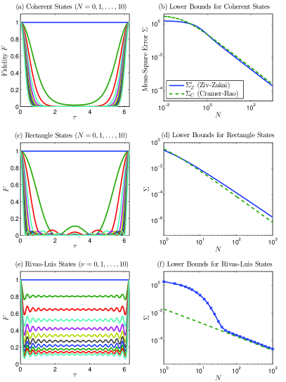
Figure 1: (Color online). Left column: fidelity of a pair of (a) coherent states, (c) rectangle states, and (e) products of Rivas-Luis states with $\epsilon=0.1$ and $N_{j}=1$ with phase difference $\tau$. Right column: mean-square-error lower bounds versus the average photon number on a log-log scale for (b) coherent states, (d) rectangle states, and (f) products of Rivas-Luis states with $\epsilon=0.1$, $N_{j}=1$, and $W=2\pi$; straight lines connecting the numerically calculated points are guides for eyes.

Next, consider the state $|\psi\rangle=(M+1)^{-1/2}\sum_{m=0}^{M}|m\rangle$, which has an equal superposition of number states up to $|M\rangle$ and shall be called the rectangle state here, with $N=M/2$ and $\Delta N^{2}=M(M+2)/12$. The QCRB given by

$$\Sigma_{C}=\frac{1}{4N(N+1)/3+\Pi}$$ (17)

follows the H-limit scaling $1/N^{2}$ for large $N$. The fidelity is $F(\tau)=\sin^{2}[(2N+1)\tau/2]/[(2N+1)^{2}\sin^{2}(\tau/2)]$. Unlike the coherent states, the fidelities for the rectangle states have sidelobes, as shown in Fig. 1(c).

The QZZB for $W=2\pi$ is sup

$$\Sigma_{Z}\geq\Sigma_{Z}^{\prime}=\frac{\pi}{2(2N+1)^{2}}\sum_{k=0}^{2N}\frac{1}{2k+1}$$

$$\to\frac{\pi\ln(4N+1)}{4(2N+1)^{2}}\textrm{ for large }N,$$ (18)

approaching a slower $\ln N/N^{2}$ scaling for large $N$. The additional factor of $\ln N$ makes the QZZB diverge from the QCRB, as shown in Fig. 1(d). The $\ln N/N^{2}$ scaling was also observed previously for the phase-squeezed state using other methods collett .

As the final example, consider the superposition of the vacuum with a state $|\zeta\rangle$ that has a large photon-number variance, viz., $|\psi\rangle_{j}=c_{0}|0\rangle+c_{1}|\zeta\rangle$ with $|c_{1}|^{2}\ll 1$, as proposed by Rivas and Luis rivas . $|\psi\rangle_{j}$ can be rewritten as $|\psi\rangle_{j}=\sqrt{1-\epsilon}|0\rangle+\sqrt{\epsilon}|\psi_{s}\rangle$, where $|\psi_{s}\rangle$ is $|\zeta\rangle$ minus the vacuum component and renormalized. If $|\psi_{s}\rangle$ has a mean photon number $N_{s}$ and photon-number variance given by $\gamma N_{s}^{2}$ with $\gamma$ a constant, the mean and variance for $|\psi\rangle_{j}$ are $N_{j}=\epsilon N_{s}$ and $\Delta N_{j}^{2}=[(1+\gamma)/\epsilon-1]N_{j}^{2}$. $\Delta N_{j}^{2}$ can be made arbitrarily larger than $N_{j}^{2}$ by reducing $\epsilon$, and the QCRB can be made arbitrarily small. With $\nu$ copies and a total photon number $N\equiv\nu N_{j}$,

$$\Sigma_{C} =\frac{1}{4[(1+\gamma)/(\nu\epsilon)-1/\nu]N^{2}+\Pi}$$ (19)

can decrease faster than the H-limit scaling $1/N^{2}$ if $\nu\epsilon$ also decreases with $N$ rivas .

The fidelity tells a very different story. Defining the fidelity for $|\psi_{s}\rangle$ as $F_{s}$, the fidelity for $|\psi\rangle_{j}$ is $F_{j}=(1-\epsilon)^{2}+2\epsilon(1-\epsilon)\langle\psi_{s}|\cos n\tau|\psi_{s}\rangle+\epsilon^{2}F_{s}\geq(1-\epsilon)^{2}-2\epsilon(1-\epsilon)=1-4\epsilon+3\epsilon^{2}$. Regardless of $|\psi_{s}\rangle$, $F_{j}$ is bounded from below by a constant close to 1 if $\epsilon\ll 1$. For $\nu$ copies, $F=F_{j}^{\nu}\geq(1-4\epsilon+3\epsilon^{2})^{\nu}$, and a bound on the QZZB follows:

$$\Sigma_{Z} \geq\frac{W^{2}}{12}\left[1-\sqrt{1-\left(1-4\epsilon+3\epsilon^{2}\right)^{\nu}}\right].$$ (20)

This bound means that the actual error cannot deviate substantially from the prior value $W^{2}/12$ until $\nu\epsilon\sim 1$, by which point even if the error catches up with the QCRB it can no longer beat the $1/N^{2}$ scaling. This result is unsurprising in light of the now proven H limit.

To study the behavior of the Rivas-Luis state in more detail, let $|\psi\rangle_{j}=\sqrt{1-\epsilon}|0\rangle+\sqrt{\epsilon/M}\sum_{m=1}^{M}|m\rangle$. Figure 1(e) plots the fidelities for some products of the Rivas-Luis states with $\epsilon=0.1$ and $N=1$, showing sharp features due to $|\psi_{s}\rangle$ near $\tau=0$ but quickly dropping off to the nonzero backgrounds due to $|0\rangle$. Figure 1(f) plots the QZZB (calculated by numerically integrating Eq. (10) with $W=2\pi$) and the QCRB given by Eq. (19) versus the total photon number $N$. The QZZB is much higher than the QCRB for small $N$ and comes down only when $N\gtrsim 10$ and $\nu\epsilon\gtrsim 1$. The QZZB then reaches a threshold, beyond which it follows closely the QCRB. This threshold behavior is encountered frequently in classical parameter estimation vantrees ; bell and also observed in a numerical study of quantum phase estimation blc .

In conclusion, the QZZBs are shown to be versatile error bounds that can predict different types of quantum limits using one unified formalism and can be much tighter than the popular QCRB for optical phase estimation in certain cases. To model quantum sensors more realistically, the QZZBs may also be generalized for waveform estimation in a way similar to the QCRB twc , if an error bound for continuous quantum hypothesis testing tsang_hypo can be found.

Discussions with L. Maccone, V. Giovannetti, M.J.W. Hall, S. Lloyd, L. Davidovich, B.M. Escher, R.L. de Matos Filho, M.G.A. Paris, Á. Rivas, A. Luis, S. Guha, A. Tacla, C.M. Caves, L.C. Kwek, A. Ling, and J.P. Dowling are gratefully acknowledged. This work is supported by the Singapore National Research Foundation under NRF Grant No. NRF-NRFF2011-07.

Appendix A Supplementary Material

This Supplementary Material contains detailed derivations of some of the results presented in the main text. Section A.1 derives the classical Ziv-Zakai bounds, Sec. A.2 calculates a quantum Ziv-Zakai bound (QZZB) when the photon-number distribution can be approximated as continuous and Gaussian, Sec. A.3 calculates the bound for coherent states, and Sec. A.4 calculates the bound for rectangle states.

A.1 Derivation of the classical Ziv-Zakai bounds

Let

$$\sigma \equiv|\tilde{X}(Y)-X|$$ (21)

be a nonnegative random variable. The mean-square error becomes

$$\Sigma =\int_{0}^{\infty}dsP_{\sigma}(s)s^{2},$$ (22)

where $P_{\sigma}(s)$ is the probability density of $\sigma$. With

$$P_{\sigma}(s) =-\frac{d}{ds}\operatorname{Pr}\left(\sigma\geq s\right)$$ (23)

and integration by parts, $\Sigma$ becomes

$$\Sigma =2\int_{0}^{\infty}dss\operatorname{Pr}\left(\sigma\geq s\right)=\frac{1}{2}\int_{0}^{\infty}d\tau\tau\operatorname{Pr}\left(|\tilde{X}-X|\geq\frac{\tau}{2}\right).$$ (24)

Since both $\tau$ and $\operatorname{Pr}(|\tilde{X}-X|\geq\tau/2)$ are nonnegative, one can find a lower bound on $\Sigma$ by bounding $\operatorname{Pr}(|\tilde{X}-X|\geq\tau/2)$. Rewrite $\operatorname{Pr}(|\tilde{X}-X|\geq\tau/2)$ as follows:

$$\operatorname{Pr}\left(|\tilde{X}-X|\geq\frac{\tau}{2}\right) =\operatorname{Pr}\left(\tilde{X}-X>\frac{\tau}{2}\right)+\operatorname{Pr}\left(\tilde{X}-X\leq-\frac{\tau}{2}\right)$$ (25)

$$=\int_{-\infty}^{\infty}dx_{0}P_{X}(x_{0})\operatorname{Pr}\left(\tilde{X}-X>\frac{\tau}{2}\bigg{|}X=x_{0}\right)$$

$$\quad+\int_{-\infty}^{\infty}dx_{1}P_{X}(x_{1})\operatorname{Pr}\left(\tilde{X}-X\leq-\frac{\tau}{2}\bigg{|}X=x_{1}\right),$$ (26)

and let

$$x_{0} =x, x_{1} =x+\tau.$$ (27)

This yields

$$\operatorname{Pr}\left(|\tilde{X}-X|\geq\frac{\tau}{2}\right) =\int_{-\infty}^{\infty}dx\bigg{[}P_{X}(x)\operatorname{Pr}\left(\tilde{X}>x+\frac{\tau}{2}\bigg{|}X=x\right)$$

$$\quad+P_{X}(x+\tau)\operatorname{Pr}\left(\tilde{X}\leq x+\frac{\tau}{2}\bigg{|}X=x+\tau\right)\bigg{]}$$ (28)

$$=\int_{-\infty}^{\infty}dx[P_{X}(x)+P_{X}(x+\tau)]$$

$$\quad\times\left\{P_{0}\operatorname{Pr}\left(\tilde{X}>x+\frac{\tau}{2}\bigg{|}X=x\right)+P_{1}\operatorname{Pr}\left(\tilde{X}\leq x+\frac{\tau}{2}\bigg{|}X=x+\tau\right)\right\},$$ (29)

where

$$P_{0} \equiv\frac{P_{X}(x)}{P_{X}(x)+P_{X}(x+\tau)}, P_{1} \equiv\frac{P_{X}(x+\tau)}{P_{X}(x)+P_{X}(x+\tau)}=1-P_{0}.$$ (30)

Now consider a binary hypothesis testing problem with hypotheses

$$\mathcal{H}_{0}:X =x, \mathcal{H}_{1}:X =x+\tau,$$ (31)

prior probabilities

$$\operatorname{Pr}(\mathcal{H}_{0}) =P_{0}, \operatorname{Pr}(\mathcal{H}_{1}) =P_{1},$$ (32)

observation probability densities

$$P_{Y}(y|\mathcal{H}_{0}) =P_{Y|X}(y|x), P_{Y}(y|\mathcal{H}_{1}) =P_{Y|X}(y|x+\tau),$$ (33)

and the following suboptimal decision rule:

$$\operatorname{choose}\mathcal{H}_{0}\operatorname{if}\tilde{X} \leq x+\frac{\tau}{2}, \operatorname{choose}\mathcal{H}_{1}\operatorname{if}\tilde{X} >x+\frac{\tau}{2}.$$ (34)

The error probability of this hypothesis testing problem is then precisely given by the expression in the curly brackets in Eq. (29). This expression is lower-bounded by the minimum error probability of the hypothesis testing problem, denoted by $\operatorname{Pr}_{e}(x,x+\tau)$, which does not depend on $\tilde{X}$, and one obtains

$$\operatorname{Pr}\left(|\tilde{X}-X|\geq\frac{\tau}{2}\right) \geq\int_{-\infty}^{\infty}dx[P_{X}(x)+P_{X}(x+\tau)]\operatorname{Pr}_{e}(x,x+\tau).$$ (35)

The left-hand side is a monotonically decreasing function of $\tau$, so a tighter bound can be obtained if we fill the valleys of the right-hand side as a function of $\tau$. Denoting this valley-filling operation as $\mathcal{V}$:

$$\mathcal{V}f(\tau) \equiv\max_{\eta\geq 0}f(\tau+\eta),$$ (36)

one gets

$$\operatorname{Pr}\left(|\tilde{X}-X|\geq\frac{\tau}{2}\right) \geq\mathcal{V}\int_{-\infty}^{\infty}dx[P_{X}(x)+P_{X}(x+\tau)]\operatorname{Pr}_{e}(x,x+\tau),$$ (37)

$$\Sigma \geq\frac{1}{2}\int_{0}^{\infty}d\tau\tau\mathcal{V}\int_{-\infty}^{\infty}dx[P_{X}(x)+P_{X}(x+\tau)]\operatorname{Pr}_{e}(x,x+\tau).$$ (38)

This is a Ziv-Zakai bound. Another version that relates the mean-square error to an equally-likely-hypothesis-testing problem can be obtained from Eq. (28):

$$\operatorname{Pr}\left(|\tilde{X}-X|\geq\frac{\tau}{2}\right) \geq\int_{-\infty}^{\infty}dx2\min[P_{X}(x),P_{X}(x+\tau)]$$

$$\quad\times\left\{\frac{1}{2}\operatorname{Pr}\left(\tilde{X}>x+\frac{\tau}{2}\bigg{|}X=x\right)+\frac{1}{2}\operatorname{Pr}\left(\tilde{X}\leq x+\frac{\tau}{2}\bigg{|}X=x+\tau\right)\right\}.$$ (39)

The expression in the curly brackets is now the error probability of the same hypothesis testing problem as before, except that the prior probabilities are

$$\operatorname{Pr}(\mathcal{H}_{0})=\operatorname{Pr}(\mathcal{H}_{1})=\frac{1}{2}.$$ (40)

Another Ziv-Zakai bound follows:

$$\Sigma \geq\frac{1}{2}\int_{0}^{\infty}d\tau\tau\mathcal{V}\int_{-\infty}^{\infty}dx2\min[P_{X}(x),P_{X}(x+\tau)]\operatorname{Pr}_{e}^{el}(x,x+\tau),$$ (41)

where $\operatorname{Pr}_{e}^{el}(x,x+\tau)$ now denotes the minimum error probability with equally likely hypotheses. Note that these bounds make no assumption about the estimate.

A.2 Quantum Ziv-Zakai bound for approximately Gaussian photon-number distributions

Consider the QZZB for optical phase estimation with a uniform prior window:

$$\Sigma_{Z} \equiv\frac{1}{2}\int_{0}^{W}d\tau\tau\left(1-\frac{\tau}{W}\right)\left[1-\sqrt{1-F(\tau)}\right],$$ (42)

$$F(\tau) \equiv\Big{|}\sum_{n}|C_{n}|^{2}\exp(in\tau)\Big{|}^{2},$$ (43)

where $|C_{n}|^{2}$ is the photon-number distribution. If $|C_{n}|^{2}$ can be approximated as a Gaussian distribution and the sum in Eq. (43) as a continuous Fourier transform,

$$|C_{n}|^{2} \approx\frac{1}{\sqrt{2\pi}\Delta N_{j}}\exp\left[-\frac{(n-N_{j})^{2}}{2\Delta N_{j}^{2}}\right],$$ (44)

$$F(\tau) \approx\Big{|}\int dn|C_{n}|^{2}\exp(in\tau)\Big{|}^{2}=\exp\left(-\Delta N_{j}^{2}\tau^{2}\right).$$ (45)

Since $1-\sqrt{1-F}\geq F/2$,

$$\Sigma_{Z} \gtrsim\frac{1}{4}\int_{0}^{W}d\tau\tau\left(1-\frac{\tau}{W}\right)F(\tau)=\frac{1}{8\Delta N_{j}^{2}}\textrm{ for }W\to\infty,$$ (46)

which is lower than the quantum Cramér-Rao bound (QCRB) by a constant factor of 2. This shows that the two bounds can differ significantly only when $|C_{n}|^{2}$ cannot be well approximated by a Gaussian.

For multiple copies, the fidelity can be written as

$$F(\tau) =\left|\sum_{n_{1},\dots,n_{\nu}}|C_{n_{1}}|^{2}|C_{n_{2}}|^{2}\dots|C_{n_{\nu}}|^{2}\exp\bigg{(}i\sum_{j}n_{j}\tau\bigg{)}\right|^{2},$$ (47)

which is the squared magnitude of the Fourier transform with respect to the total photon number $\sum_{j}n_{j}$. By virtue of the central limit theorem, the total-photon-number statistics will become approximately Gaussian with variance $\nu\Delta N_{j}^{2}$ in the limit of large $\nu$. This means that, regardless of the form of $|C_{n}|^{2}$, the QZZB and the QCRB will become comparable in the limit of large $\nu$.

A.3 Quantum Ziv-Zakai bound for coherent states

With the inequalities

$$\tau\left(1-\frac{\tau}{W}\right) \geq\frac{W}{4}\sin\frac{\pi\tau}{W}, 0 \leq\tau\leq W,$$ (48)

$$1-\sqrt{1-F} \geq\frac{1}{2}F, 0 \leq F\leq 1,$$ (49)

the QZZB becomes

$$\Sigma_{Z} \equiv\frac{1}{2}\int_{0}^{W}d\tau\tau\left(1-\frac{\tau}{W}\right)\left[1-\sqrt{1-F(\tau)}\right]$$ (50)

$$\geq\frac{W}{16}\int_{0}^{W}d\tau\sin\frac{\pi\tau}{W}F(\tau).$$ (51)

For a coherent state and $W=2\pi$,

$$\Sigma_{Z} \geq\frac{\pi}{8}\exp(-2N)\int_{0}^{2\pi}d\tau\sin\frac{\tau}{2}\exp\left(2N\cos\tau\right).$$ (52)

Changing the integration variable to $u\equiv\cos(\tau/2)$ and using the identity $\cos\tau=2\cos^{2}(\tau/2)-1$, one obtains

$$\Sigma_{Z} \geq\frac{\pi}{2}\exp(-4N)\int_{-1}^{1}du\exp(4Nu^{2}),$$ (53)

which leads to Eq. (16) in the text.

A.4 Quantum Ziv-Zakai bound for rectangle states

Using Eq. (51) with $W=2\pi$, one obtains

$$\Sigma_{Z} \geq\frac{\pi}{8(M+1)^{2}}I_{M},$$ (54)

$$I_{M} \equiv\int_{0}^{2\pi}d\tau\frac{\sin^{2}(M+1)\tau/2}{\sin\tau/2}.$$ (55)

It can be shown using trigonometric identities that

$$\sin^{2}\frac{(M+1)\tau}{2} =\sin^{2}\frac{(M-1)\tau}{2}+4\sin\frac{\tau}{2}\cos\frac{M\tau}{2}\sin\frac{(M-1)\tau}{2}+4\sin^{2}\frac{\tau}{2}\cos^{2}\frac{M\tau}{2}.$$ (56)

The integral $I_{M}$ then satisfies the recursive relation

$$I_{M} =I_{M-2}+\frac{16M}{(2M-1)(2M+1)}$$ (57)

$$=I_{M-2}+4\left[\frac{1}{2(M-1)+1}+\frac{1}{2M+1}\right],$$ (58)

with $I_{-1}=0$ and $I_{0}=4$. Hence

$$I_{M} =4\sum_{k=0}^{M}\frac{1}{2k+1}.$$ (59)

For large $M$, the discrete sum can be approximated by an integral:

$$I_{M} \approx 4\int_{0}^{M}dk\frac{1}{2k+1}=2\ln(2M+1).$$ (60)

References

(1)H. L. Van Trees,
Detection, Estimation, and Modulation Theory, Part I
(Wiley, New York, 2001).
(2)H. L. Van Trees and K. L. Bell (Eds.),
Bayesian Bounds for Parameter Estimation and Nonlinear Filtering/Tracking
(Wiley-IEEE, Piscataway, 2007), and references therein.
(3)J. Ziv and M. Zakai,
IEEE Trans. Inform. Theor. IT-15, 386 (1969);
L. P. Seidman,
Proc. IEEE 58, 644 (1970);
D. Chazan, M. Zakai, and J. Ziv,
IEEE Trans. Inform. Theor. IT-21, 90 (1975);
S. Bellini and G. Tartara,
IEEE Trans. Commun. COM-22, 340 (1974);
E. Weinstein,
IEEE Trans. Inform. Theor. 34, 342 (1988).
(4)
D. Nicholson and A. Vecchio,
Phys. Rev. D57, 4588 (1998);
K. J. Lee et al.,
Mon. Not. R. Astron. Soc. 414, 3251 (2011).
(5)V. Giovannetti, S. Lloyd, and L. Maccone,
Science 306, 1330 (2004);
Nature Photon. 5, 222 (2011).
(6)C. W. Helstrom,
Quantum Detection and Estimation Theory
(Academic Press, New York, 1976);
A. S. Holevo,
Probabilistic and Statistical Aspects of Quantum Theory
(North-Holland, Amsterdam, 1982);
H. M. Wiseman and G. J. Milburn,
Quantum Measurement and Control
(Cambridge University Press, Cambridge, 2010).
(7)H. P. Yuen and M. Lax,
IEEE Trans. Inform. Theor. IT-19, 740 (1973).
(8)M. Tsang, H. M. Wiseman, and C. M. Caves,
Phys. Rev. Lett. 106, 090401 (2011).
(9)
This Letter defines the tightness of a bound by
comparing the bound to the achievable error.
A QCRB is always less tight to the error than the classical CRB
for a particular measurement strategy; see
S. L. Braunstein and C. M. Caves,
Phys. Rev. Lett. 72, 3439 (1994).
This has motivated many studies
[see, for example, M. G. Genoni, S. Olivares, and M. G. A. Paris,
Phys. Rev. Lett. 106, 153603 (2011)]
that analyze the tightness of a QCRB relative to a classical CRB,
but the QCRB cannot be tight to the error if the classical CRB is not.
(10)
J. H. Shapiro, S. R. Shepard, and N. C. Wong,
Phys. Rev. Lett. 62, 2377 (1989);
J. H. Shapiro and S. R. Shepard,
Phys. Rev. A43, 3795 (1991).
(11)
P. M. Anisimov et al.,
Phys. Rev. Lett. 104, 103602 (2010);
Y. R. Zhang et al.,
e-print arXiv:1105.2990.
(12)Á. Rivas and A. Luis,
e-print arXiv:1105.6310.
(13)S. L. Braunstein, A. S. Lane, and C. M. Caves,
Phys. Rev. Lett. 69, 2153 (1992).
(14)
M. Genoni et al., e-print arXiv:1203.2956.
(15)M. G. A. Paris,
Phys. Lett. A 225, 23 (1997);
Z. Y. Ou, Phys. Rev. Lett. 77, 2352 (1996).
(16) It is unfortunate that this limit has come to be
known as the Heisenberg limit in the literature, as it is
fundamentally different from the Heisenberg uncertainty relation,
which is a relation of variances.
(17)
B. Yurke, S. L. McCall, J. R. Klauder,
Phys. Rev. A33, 4033 (1986);
B. C. Sanders and G. J. Milburn,
Phys. Rev. Lett. 75, 2944 (1995);
Z. Y. Ou,
Phys. Rev. Lett. 77, 2352 (1996);
Phys. Rev. A55, 2598 (1997);
J. J. Bollinger, W. M. Itano, D. J. Wineland,
and D. J. Heinzen,
Phys. Rev. A54, R4649 (1996);
P. Hyllus, L. Pezzé, and A. Smerzi,
Phys. Rev. Lett. 105, 120501 (2010);
M. Zwierz, C. A. Peŕez-Delgado, and P. Kok,
Phys. Rev. Lett. 105, 180402 (2010);
107, 059904(E) (2011).
(18)V. Giovannetti, S. Lloyd, and L. Maccone,
e-print arXiv:1109.5661.
(19)
M. J. W. Hall, D. W. Berry, M. Zwierz, and H. M. Wiseman,
Phys. Rev. A85, 041802(R) (2012);
M. J. W. Hall,
J. Mod. Opt. 40, 809 (1993).
(20)See Supplementary Material for detailed calculations.
(21)C. A. Fuchs and J. van de Graaf,
IEEE Trans. Inform. Theor. 45, 1216 (1999).
(22)S. L. Braunstein, C. M. Caves, and
G. J. Milburn,
Ann. Phys. 247, 135 (1996).
(23)
V. Giovannetti, S. Lloyd, and L. Maccone,
Phys. Rev. A67, 052109 (2003).
(24)S. Boixo, S. T. Flammia, C. M. Caves,
and J. M. Geremia,
Phys. Rev. Lett. 98, 090401 (2007).
(25) G. H. Fleming,
Nuovo Cimento 16A, 232 (1973).
(26)M. J. Collett,
Physica Scripta T48, 124 (1993);
H. M. Wiseman and R. B. Killip,
Phys. Rev. A57, 2169 (1998);
D. W. Berry and H. M. Wiseman,
Phys. Rev. A63, 013813 (2000);
M. Tsang, J. H. Shapiro, and S. Lloyd,
Phys. Rev. A78, 053820 (2008); 79, 053843 (2009).
(27)M. Tsang,
Phys. Rev. Lett. 108, 170502 (2012).