Tunneling theory of two interacting atoms in a trap

Abstract

A theory for the tunneling of one atom out of a trap containing two interacting cold atoms is developed. The quasiparticle wave function, dressed by the interaction with the companion atom in the trap, replaces the non-interacting orbital at resonance in the tunneling matrix element. The computed decay time for two ⁶Li atoms agrees with recent experimental results [G. Zürn, F. Serwane, T. Lompe, A. N. Wenz, M. G. Ries, J. E. Bohn, and S. Jochim, arXiv:1111.2727], unveiling the ‘fermionization’ of the wave function and a novel two-body effect.

Recently few cold atoms have been confined in tight single optical traps with control of their number and quantum states Cheinet08 ; Serwane11 . This capability is exciting as it bridges different fields such as mesoscopic and nuclear physics. Systems made of just two interacting atoms are especially relevant, being the building blocks of many-body strongly correlated states BlochRMP and allowing for comparison with fully understood theoretical models Busch ; Girardeau10 .

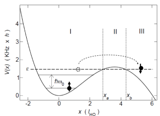
Figure 1: Confinement potential $V(x)$ vs $x$ according to Ref. Zuern11, . The harmonic oscillator frequency $\omega_{0}=$ 0.744 KHz$\cdot 2\pi$ is obtained from the spacing between the two bound states of $V(x)$ computed through the WKB approximation (solid thin lines); $\varepsilon$ is the resonating tunneling energy. The length unit is $\ell_{\text{HO}}=(\hbar/m\omega_{0})^{1/2}$. The circles with arrows schematize the atoms in the $\left|\uparrow\downarrow\right>$ configuration.

In a fascinating experiment Zuern11 , the Heidelberg group has prepared in a one-dimensional trap (Fig. 1) two ⁶Li atoms behaving as fermions of spin one-half and interacting through a tunable contact potential, $g\,\delta(x_{1}-x_{2})$. The $\left|\uparrow\uparrow\right>$ ($\left|\downarrow\downarrow\right>$) state has a fermionic-like orbital wave function, being odd under particle exchange, $\psi_{\uparrow\uparrow}(x_{1},x_{2})=-\psi_{\uparrow\uparrow}(x_{2},x_{1})$, whereas the $\left|\uparrow\downarrow\right>$ wave function is bosonic-like, $\psi_{\uparrow\downarrow}(x_{1},x_{2})=\psi_{\uparrow\downarrow}(x_{2},x_{1})$. The time $\tau$ spent by one atom to tunnel out of the trap is measured as a function of the interaction strength $g$. As shown in Fig. 2, at $g=\infty$ the decay time $\tau$ is the same for both $\left|\uparrow\downarrow\right>$ and $\left|\uparrow\uparrow\right>$ ($\left|\uparrow\uparrow\right>$, being non-interacting, is independent from $g$). The coincidence of $\tau$ is attributed to the Fermi-Bose duality (FBD, aka ‘fermionization’) Girardeau60 ; duality ; delCampo , i.e., the energy and wave function modulus of $\left|\uparrow\downarrow\right>$ are the same as $\left|\uparrow\uparrow\right>$, $\left|\psi_{\uparrow\downarrow}(x_{1},x_{2})\right|^{2}=\left|\psi_{\uparrow\uparrow}(x_{1},x_{2})\right|^{2}$. This duality was predicted long ago for the Tonks-Girardeau (TG) gas Girardeau60 and it has been demonstrated for repulsively interacting bosons repbos . At finite $g$ both TG ($g>0$) and super-TG ($g<0$) states Girardeau10 ; Tempfli09 of $\left|\uparrow\downarrow\right>$ are accessed, the former being the ground state and the latter the first excited state, here stabilized by the absence of three-body collisions Zuern11 .

The experiment raises two issues: (i) A rigorous argument for the coincidence of $\tau$ was not given. In fact, the FBD applies only to those observables that involve the wave function square modulus Girardeau60 , whereas $\tau$ originates from the convolution of orbital states inside and outside the trap Bardeen61 . Indeed, in two dimensions $\tau$ may depend on the wave function phase Lorke10 ; Rontani11 . (ii) So far $\tau$ has been computed using a single-particle theory Zuern11 , including the effect of interactions through energy renormalization [black dashed lines in Fig. 2(a)]. As the agreement with the experimental data (points) is qualitative, question arises whether the shape of the interacting wave function may affect $\tau$.

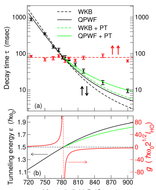
Figure 2: (Color online) (a) Decay time $\tau$ vs magnetic field $B$. The points with error bars are the experimental data Zuern11 , the dashed and solid lines are respectively the WKB ($\tau_{0}$) and QPWF predictions. The green [light gray] lines include the PT correction to the tunneling energy $\varepsilon$. (b) Interaction strength $g$ (red [gray] curve) and $\varepsilon$ (black and green [light gray] curve) vs $B$. $g$ is taken from Ref. Zuern11, and $\varepsilon$ is computed after Ref. Busch, (black curve). The green (light gray) line includes the PT correction. The dashed lines are guides to the eye.

In this Letter a theory of tunneling for two interacting atoms is developed, based on the calculation of the quasiparticle wave function (QPWF) Rontani05 ; Toroz11 . The QPWF is the interacting counterpart of the single-particle orbital resonating at the energy $\varepsilon$ of the atom tunneling out of the trap, dressed by the interaction with the companion atom. At $g=\infty$, the QPWFs of both $\left|\uparrow\downarrow\right>$ and $\left|\uparrow\uparrow\right>$ are found to be identical in the tunnel barrier [Fig. 3(f)], hence the decay times $\tau$ coincide. At finite $g$, $\tau$ is evaluated numerically from the exact wave function for harmonic confinement Busch plus perturbation theory (PT) to account for the anharmonic terms of the potential trap. The two-body correction significantly improves the agreement with experimental data [solid lines in Fig. 2(a)], illustrating a novel few-body effect, similar to orthogonality catastrophe Anderson .

The starting point of the theory is the Hamiltonian

$$H=-\frac{\hbar^{2}}{2m}\sum_{i=1}^{2}\left[\frac{d^{2}}{dx_{i}^{2}}+V(x_{i})\right]+g\delta(x_{1}-x_{2}),$$ (1)

with $m$ being the mass and $V(x)$ an effective one-dimensional potential. The plot of $V(x)$ in Fig. 1 reproduces the setup of Ref. Zuern11, . Atom-atom interaction is neglected outside the trap, that is approximately parabolic at low energy. Here the two atoms are either spin-1/2 fermions or spinless bosons. The treatment for bosons is the same as for $\left|\uparrow\downarrow\right>$, hence only fermions are considered.

Following Bardeen Bardeen61 , the space is divided into three regions: the trap (I), the barrier (II), and the vacuum (III) (Fig. 1). The boundaries are the classical turning points $x_{a}$ and $x_{b}$, hence region II extends from $x_{a}$ to $x_{b}$. There are two classes of single-particle states:
(i) Vacuum stationary waves $\chi_{\varepsilon}(x)$ of (continuous) energy $\varepsilon$. These are plane waves in region III reflected at the barrier and dropping exponentially with distance into region II. For example, in the WKB approximation one has $\chi_{\varepsilon}(x)=Ck(x)^{-1/2}\cos{(\int_{x_{b}}^{x}\!\!k(x^{\prime})dx^{\prime}-\pi/4)}$ for $x>x_{b}$ and $\chi_{\varepsilon}(x)=Ck(x)^{-1/2}2^{-1}\exp{(-\int_{x}^{x_{b}}\!\!k(x^{\prime})dx^{\prime})}$ for $x_{a}<x<x_{b}$, where $C$ is a normalization constant and $k(x)=[(2m/\hbar^{2})\left|\varepsilon-V(x)\right|]^{1/2}$. For $x<x_{a}$ $\chi_{\varepsilon}(x)$ drops smoothly to zero, instead of oscillating, so $\chi_{\varepsilon}(x)$ is not a good solution for $x<x_{a}$.
(ii) Trap eigenstates $\phi_{n}(x)$ ($n=0,1,2,\ldots$), which have a vanishing tail in region II and smoothly go to zero in region III. In region I $\phi_{n}(x)$ is approximately an eigenstate of the harmonic oscillator (HO) with energy $\hbar\omega_{0}(n+1/2)$.
To summarize, trap states are solutions of the single-particle Schrödinger equation in regions I and II but not in III, whereas stationary waves are solutions in regions II and III but not in I. Therefore, none of the above states are eigenstates in the whole space, but they are approximately orthogonal.

Similarly, $\Psi_{0}(x_{1},x_{2})$ and $\Psi_{m,\varepsilon}(x_{1},x_{2})$ are states of the entire system with two fermions that differ in the transfer of an atom from region I to region III. $\Psi_{0}(x_{1},x_{2})$ has two atoms in the trap, either distinguishable ($\Psi_{0}=\psi_{\uparrow\downarrow}$) or indistinguishable ($\Psi_{0}=\psi_{\uparrow\uparrow}$ or $\psi_{\downarrow\downarrow}$). The latter are non interacting as $\psi_{\uparrow\uparrow}(x,x)=0$ for symmetry. $\Psi_{m,\varepsilon}$ is the non-interacting state with one atom left in the trap orbital $\phi_{m}(x)$ and the other one transferred to the vacuum state $\chi_{\varepsilon}(x)$ (Fig. 1 depicts $\Psi_{0,\varepsilon}$). Thus $\Psi_{0}$ is a solution of the interacting Schrödinger equation with energy $W_{0}$ in region I and II but not in III, and $\Psi_{m,\varepsilon}$ is a solution with energy $W_{m,\varepsilon}$ in region II and III but not in I. Both $\Psi_{0}$ and $\Psi_{m,\varepsilon}$ are good solutions in region II.

Bardeen has shown Bardeen61 that the matrix element $M_{m,\varepsilon}$ for the transition from $\Psi_{0}$ to $\Psi_{m,\varepsilon}$, as long as the energy is conserved ($W_{0}\approx W_{m,\varepsilon})$, is $M_{m,\varepsilon}=-\hbar^{2}J_{m,\varepsilon}/2m$, with $J_{m,\varepsilon}$ being proportional to the matrix element of the probability current density operator,

$$J_{m,\varepsilon}=\sum_{i=1}^{2}\int_{-\infty}^{\infty}\!\!\!\!\!\!\!\!dx_{1}\!\!\int_{-\infty}^{\infty}\!\!\!\!\!\!\!\!dx_{2}\,\,\delta(x_{i}-x_{\text{bar}})\!\left[\Psi_{0}^{*}\frac{d\Psi_{m,\varepsilon}}{dx_{i}}-\Psi_{m,\varepsilon}\frac{d\Psi_{0}^{*}}{dx_{i}}\right],$$ (2)

and $x_{\text{bar}}$ being any point in the barrier region II. It is implicit in Eq. (2) that $\Psi_{0}$ and $\Psi_{m,\varepsilon}$ have the same spinorial component as tunneling does not affect spin. The decay rate $1/\tau$ may be estimated from Fermi golden rule,

$$\frac{1}{\tau}=\frac{2\pi}{\hbar}\sum_{m,\varepsilon}\left|M_{m,\varepsilon}\right|^{2}\delta(W_{0}-W_{m,\varepsilon}).$$ (3)

The non-interacting case $\left|\uparrow\uparrow\right>$ is easy to work out. The trap ground state $\Psi_{0}$ is the Slater determinant of the $(n=0)(n=1)$ configuration,

$$\psi_{\uparrow\uparrow}(x_{1},x_{2})=\frac{1}{\sqrt{2}}\left[\phi_{0}(x_{1})\phi_{1}(x_{2})-\phi_{0}(x_{2})\phi_{1}(x_{1})\right].$$

Among possible final states, the most relevant one is the $(n=0)(\varepsilon=3\hbar\omega/2)$ configuration $\Psi_{0,\varepsilon}$,

$$\Psi_{0,\varepsilon}(x_{1},x_{2})=\frac{1}{\sqrt{2}}\left[\phi_{0}(x_{1})\chi_{\varepsilon}(x_{2})-\phi_{0}(x_{2})\chi_{\varepsilon}(x_{1})\right],$$

providing the transfer matrix element $J_{0,3\hbar\omega/2}$,

$$J_{0,3\hbar\omega/2}=\left[\phi_{1}^{*}(x)\frac{d\chi_{\varepsilon}(x)}{dx}-\chi_{\varepsilon}(x)\frac{d\phi_{1}^{*}(x)}{dx}\right]_{x=x_{\text{bar}}}^{\varepsilon=3\hbar\omega/2}.$$ (4)

Equation (4) is the obvious non-interacting result for resonant tunneling between the highest occupied orbital of the trap, $\phi_{1}(x)$, and the vacuum state, $\chi_{\varepsilon=3\hbar\omega/2}(x)$, with the other spectator atom frozen in the orbital $\phi_{0}(x)$ of the trap. In principle, there are final states other than $\Psi_{0,3\hbar\omega/2}$ allowed by energy conservation, like the $(n=1)(\varepsilon=\hbar\omega/2)$ configuration. However, the corresponding matrix elements are negligible since wave function tails drop exponentially with energy in the barrier.

The case of two distinguishable fermions is not trivial, as $\psi_{\uparrow\downarrow}(x_{1},x_{2})$ may not be written as a single Slater determinant. Nevertheless, the exact analytical solution is available in the relative-motion frame Busch ; Girardeau10 . Explicitly,

$$\psi_{\uparrow\downarrow}(x_{1},x_{2})=\Psi_{\text{CM}}([x_{1}+x_{2}]/2)\Psi_{r}(x_{1}-x_{2}),$$ (5)

with $\Psi_{\text{CM}}$ and $\Psi_{r}$ being functions of the center-of-mass and relative-motion coordinates, respectively. Since the singlet spin part is an odd function under particle exchange, $\Psi_{r}$ must be even, as shown in Fig. 3 (red [gray] curves), where $\Psi_{r}(x)$ is plotted for various interaction strengths $g$. Note that $\Psi_{r}(x)$ has two nodes for $g<0$ (super-TG regime). The wave function $\Psi_{\text{CM}}$ is just the lowest HO state in the center-of-mass frame.

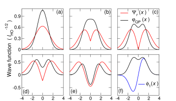
Figure 3: (Color online) Quasiparticle wave function $\varphi_{\text{QP}}(x)$ (black curves) and relative-motion wave function $\Psi_{r}(x)$ (red [gray] curves) of $\left|\uparrow\downarrow\right>$ at various $g$. (a) $g=0+$. (b) $g/(2^{1/2}\hbar\omega_{0}\ell_{\text{HO}})=3.14$. (c) $g=\infty$. (d) $g/(2^{1/2}\hbar\omega_{0}\ell_{\text{HO}})=-3.77$. (e) $g=0-$. (f) The first excited state of the harmonic oscillator, $\phi_{1}(x)$ (blue [dark gray] curve), being the QPWF of $\left|\uparrow\uparrow\right>$, is compared with $\varphi_{\text{QP}}(x)$ of $\left|\uparrow\downarrow\right>$ at $g=\infty$.

The final state $\Psi_{0,\varepsilon}$ is again a spin singlet, with an atom left in the trap lowest orbital $\phi_{0}(x)$ and the other one transferred into the vacuum state $\chi_{\varepsilon}(x)$,

$$\Psi_{0,\varepsilon}(x_{1},x_{2})=\frac{1}{\sqrt{2}}\left[\phi_{0}(x_{1})\chi_{\varepsilon}(x_{2})+\phi_{0}(x_{2})\chi_{\varepsilon}(x_{1})\right].$$ (6)

Here the resonance energy $\varepsilon$ is fixed by energy conservation. $\varepsilon$ is plotted in Fig. 2(b) (black curve) as a function of the magnetic field $B$ that controls the interaction strength $g$ (red [gray] curve) in the experiment.

By inserting expressions (5) and (6) into (2) one obtains the important result

$$J_{0,\varepsilon}=\left[\varphi_{\text{QP}}^{*}(x)\frac{d\chi_{\varepsilon}(x)}{dx}-\chi_{\varepsilon}(x)\frac{d\varphi_{\text{QP}}^{*}(x)}{dx}\right]_{x=x_{\text{bar}}},$$ (7)

with $\varphi_{\text{QP}}(x)$ being the QPWF of the atom escaping from the trap, defined as

$$\varphi_{\text{QP}}(x)=\sqrt{2}\int_{-\infty}^{\infty}\!\!dx^{\prime}\phi_{0}(x^{\prime})\Psi^{*}_{\text{CM}}([x^{\prime}+x]/2)\Psi^{*}_{r}(x^{\prime}-x).$$ (8)

From the comparison of Eq. (7) and (4) it is clear that, even in the presence of interaction, the tunneling is due to the resonance between the vacuum state $\chi_{\varepsilon}(x)$ and the quasiparticle state $\varphi_{\text{QP}}(x)$. With respect to the non-interacting case of indistinguishable fermions, $\varphi_{\text{QP}}(x)$ generalizes the role of the highest occupied orbital $\phi_{1}(x)$. Conversely, $\phi_{1}(x)$ is the QPWF of the trivial $\left|\uparrow\uparrow\right>$ case.

At infinite interaction, $g=\infty$, $\Psi_{r}(x)$ is ‘fermionized’ [red (gray) curve in Fig. 3(c)]. This means that $\Psi_{r}(x)$ overlaps with the modulus of the wave function of the non-interacting state $\left|\uparrow\uparrow\right>$. The latter is just $\left|\phi_{1}\!(x)\right|$ in the relative-motion frame. The QPWF of $\left|\uparrow\downarrow\right>$ becomes

$$\varphi_{\text{QP}}(x)=\frac{2^{1/2}}{\pi^{3/4}\ell_{\text{HO}}^{5/2}}e^{-x^{2}/2\ell_{\text{HO}}^{2}}\quad\times$$

$$\left[\int_{x}^{\infty}\!\!\!\!\!\!dx^{\prime}e^{-x^{\prime 2}/\ell_{\text{HO}}^{2}}(x^{\prime}-x)+\!\!\int_{-\infty}^{x}\!\!\!\!\!\!dx^{\prime}e^{-x^{\prime 2}/\ell_{\text{HO}}^{2}}(x-x^{\prime})\right],$$ (9)

with $\ell_{\text{HO}}=(\hbar/m\omega_{0})^{1/2}$ being the HO length in the laboratory frame. From Fig. 3(f) it is patent that $\varphi_{\text{QP}}(x)$ (black curve) is unrelated to $\phi_{1}(x)$ in the laboratory frame (blue [gray] curve), i.e., the QPWF of $\left|\uparrow\uparrow\right>$. Indeed, $\varphi_{\text{QP}}(x)$ is an even function, with opposite peaks separated by a valley with significant weight in the center, whereas $\phi_{1}(x)$ has a node.

However, if $x$ is in the potential barrier the first integral between square brackets in Eq. (9) may be neglected and the second one integrated over the whole space. This immediately provides $\varphi_{\text{QP}}(x_{\text{bar}})\cong\phi_{1}(x_{\text{bar}})$. As it may be checked visually in Fig. 3(f), this approximate identity is very well satisfied in region II. Since the energies $\varepsilon=3\hbar\omega_{0}/2$ of both QPWFs are the same, it follows that the transfer matrix elements (4) and (7) are identical and hence the decay times $\tau$, in agreement with the experimental data (circles with error bars) shown in Fig. 2(a).

The inspection of Figs. 3(a-e) over the whole range of $g$ reveals that $\varphi_{\text{QP}}(x)$ is an amplitude distibution conceptually different from $\Psi_{r}(x)$. This is evident from the very fact that the two functions have separate natural frames, respectively the laboratory and the relative-motion frame (note the distinct lateral sizes in Fig. 3). The form of $\varphi_{\text{QP}}(x)$ in the non interacting limits $g=0+$ and $g=0-$ may be derived explicitly, providing respectively $\sqrt{2}\phi_{0}(x)$ [Fig. 3(a)] and $\phi_{2}(x)/\sqrt{2}$ [Fig. 3(e)]. Overall, $\varphi_{\text{QP}}(x)$ smoothly interpolates between these two limits as $1/g$ goes from $+\infty$ to $-\infty$.

The magnitude of $\tau$ depends on the tail of $\varphi_{\text{QP}}(x)$ in the potential barrier [Eq. (7)]. Since there the QPWF profile is similar to those of non-interacting HO orbitals, it may seem that interaction affects $\tau$ only by renormalizing the tunneling energy $\varepsilon$. This is incorrect, as the norm $A_{\text{QP}}$ of the QPWF, $A_{\text{QP}}=\int dx\left|\varphi_{\text{QP}}(x)\right|^{2}$, varies strongly with the interaction strength. In fact, $A_{\text{QP}}$ decreases monotonously from the value 2 at $1/g=+\infty$ down to 1/2 at $1/g=-\infty$, being one at $1/g=0$.

Therefore, the decay rate $1/\tau$ of Eq. (3) may be approximately written as

$$\frac{1}{\tau}\cong\frac{A_{\text{QP}}}{\tau_{0}},$$ (10)

with the following provisos: (i) only one final state is considered, resonating at the energy $\varepsilon$ fixed by the interaction strength $g$; (ii) $\tau_{0}$ is the decay time obtained in the absence of interaction for elastic tunneling at energy $\varepsilon$; (iii) $A_{\text{QP}}$ is the norm of the QPWF whose energy is $\varepsilon$.

Figure 2(a) shows the single-particle decay time $\tau_{0}$ (dashed lines) as a function of $B$ (interaction strength) evaluated through the WKB formula used in Ref. Zuern11, ,

$$\frac{1}{\tau_{0}}=\frac{\varepsilon}{2\pi\hbar}\exp{\left(-2\!\!\int_{x_{a}}^{x_{b}}\!\!\!k(x)dx\right)}.$$ (11)

In this approximation $\tau_{0}$ depends only on $\varepsilon$ and the shape of $V(x)$. For $\left|\uparrow\uparrow\right>$, $\tau_{0}$ is independent from $B$ which was also observed in the experiment [red (gray) circles with error bars in Fig. 2(a)], being the state non-interacting. For $\left|\uparrow\downarrow\right>$ (black dashed lines and circles) the agreement is only qualitative, with $\tau_{0}$ spanning three decades in the 1-1000 msec range and decreasing with increasing energy. The departure of $\tau_{0}$ from the measured time is systematic, with a blueshift on the repulsive side with the largest error of $45\%$ at $B=725$ G, and a redshift on the attractive side, with an error of $65\%$ at 900 G.

The QPWF correction based on Eq. (10) improves significantly the agreement between the predicted [solid black lines in Fig. 2(a)] and measured (black circles) values of $\tau$ on the positive side Lode09 ; Kim11 of the interaction strength $g$, as the matching is almost within the error bars. On the negative side the estimated value of $\tau$ is strongly blueshifted with respect to $\tau_{0}$, with a residual error of 40% at $B=900$ G. Such discrepancy originates from the difference between the actual potential $V(x)$ shown in Fig. 1 and the harmonic trap $V_{\text{HO}}(x)=m\omega_{0}^{2}(x-x_{0})^{2}/2$ used to compute $\varepsilon$ Busch , the higher the energy the stronger the anharmonicity.

By employing PT to first order in $V(x)-V_{\text{HO}}(x)$, one may evaluate the correction $\Delta\varepsilon$ to $\varepsilon$, as shown in Fig. 2(b) (green [light gray] curve). Here the free parameter $x_{0}=0.659\ell_{\text{HO}}$ has been fixed by minimizing $\Delta\varepsilon$ at $g=\infty$ and the resulting small value $\Delta\varepsilon=0.02\hbar\omega_{0}$ has been rigidly offset at any $g<0$. Note that $\Delta\varepsilon\ll\hbar\omega_{0}$ in the considered range of $B$, justifying the usage of PT a posteriori. The value of $\varepsilon$ corrected by PT is then used to compute $\tau_{0}$ through Eq. (11) [dashed green (light gray) line in Fig. 2(a)] and $\tau$ through (10) [solid green (light gray) line]. Now the predicted value of $\tau$ satisfactorily reproduces the experimental data, uncovering the two-body effect inherent in the loss of weight of the QPWF.

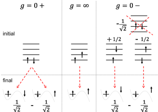
Figure 4: (Color online) Expansion of two-fermion states at various interaction strengths $g$ on the basis of the Slater determinants obtained by filling with the atoms the orbitals of the harmonic oscillator (depicted as a ladder) and the stationary waves in the vacuum. The numbers are the pertinent expansion coefficients. No label means a unity coefficient. The dashed red [gray] arrows point to the allowed tunneling transitions between initial and final configurations.

The norm $A_{\text{QP}}$ of the QPWF measures the matching of the initial two-atom state $\Psi_{0}$ with that obtained by letting the current operator act on the final state $\Psi_{0,\varepsilon}$. To understand the evolution of $A_{\text{QP}}$ with $g$ it is useful to write $\Psi_{0}$ in the laboratory frame. The simplest case of $\left|\uparrow\uparrow\right>$ is schematized in the center column of Fig. 4. The initial state is a Slater determinant with one atom in $\phi_{0}(x)$ and the other one in $\phi_{1}(x)$; the final state has one atom in $\phi_{0}(x)$ and one in $\chi_{\varepsilon}(x)$. The coefficients of both determinants are one. The two states overlap if one transfers one atom from $\phi_{1}(x)$ into $\chi_{\varepsilon}(x)$, as indicated by the dashed arrow. This single-particle result may be taken as a reference, providing a unity contribution to the tunneling matrix element. This discussion holds also for $\left|\uparrow\downarrow\right>$ at $g=\infty$.

The continuous evolution of $A_{\text{QP}}$ from $g=-\infty$ to $g=0-$ may be understood by considering the limit of $g=0-$, depicted in the right column of Fig. 4 (not accessible in the experiment). Three different configurations span $\Psi_{0}$ in the lab frame: the two atoms either doubly occupy $\phi_{1}(x)$ or singly occupy $\phi_{0}(x)$ and $\phi_{2}(x)$ with alternate spins. However, only the latter configurations are effective in transferring the atom from $\phi_{2}(x)$ into $\chi_{\varepsilon}(x)$, providing two non-zero spin-conserving contributions, each of weight $1/2\times 1/\sqrt{2}$. The total contribution to the squared matrix element is 1/2. Such decrease of the QPWF weight, arising from the multiple configurations that generically span a many-body state, is familiar from the field of strongly correlated electrons interacting through Coulomb repulsive forces Rontani05 .

The positive branch of $g$ shows a more exotic behavior. In the limit $g=0+$ (left column of Fig. 4) $\Psi_{0}$ is a non-interacting configuration with $\phi_{0}(x)$ being doubly occupied. This single configuration contributes twice to the final state, as both atoms may tunnel with opposite spins ($2\times 1/\sqrt{2}$). Therefore, the square matrix element is doubled. This coefficient may be regarded as a bosonic-like enhancement factor. Indeed, $\psi_{\uparrow\downarrow}(x_{1},x_{2})$ is the wave function of two spinless non-interacting bosons, both occupying the level $\phi_{0}(x)$.

In conclusion, the quasiparticle theory of tunneling here developed explains the available experimental data for two ⁶Li atoms. The comparison with measured decay times discloses a genuine two-body effect, related to the actual form of the interacting wave function. Therefore, such measurements may be regarded as a novel type of spectroscopy for cold atoms, paralleling successful techniques of condensed matter, such as photoemission and single-electron tunneling.

- (1) P. Cheinet, S. Trotzky, M. Feld, U. Schnorrberger, M. Moreno-Cardoner, S. Fölling, and I. Bloch, Phys. Rev. Lett. 101, 090404 (2008).
- (2) F. Serwane, G. Zürn, T. Lompe, T. B. Ottenstein, A. N. Wenz, and S. Jochim, Science 332, 336 (2011).
- (3) I. Bloch, J. Dalibard, and W. Zwerger, Rev. Mod. Phys. 80, 885 (2008); S. Giorgini, L. P. Pitaevskii, and S. Stringari, ibid. 80, 1215 (2008).
- (4) T. Busch, B.-G. Englert, K. Rza̧żewski, and M. Wilkens, Found. Phys. 28, 549 (1998).
- (5) M. D. Girardeau and G. E. Astrakharchik, Phys. Rev. A 81, 061601(R) (2010); ibid. M. D. Girardeau, 82, 011607(R) (2010).
- (6) G. Zürn, F. Serwane, T. Lompe, A. N. Wenz, M. G. Ries, J. E. Bohn, and S. Jochim, arXiv:1111.2727.
- (7) M. Girardeau, J. Math. Phys. 1, 516 (1960).
- (8) T. Cheon and T. Shigehara, Phys. Rev. Lett. 82, 2536 (1999).
- (9) A. del Campo, F. Delgado, G. García-Calderón, J. G. Muga, and M. G. Raizen, Phys. Rev. A 74, 013605 (2006).
- (10) T. Kinoshita, T. Wenger, and D. S. Weiss, Science 305, 1125 (2004); B. Paredes, A. Widera, V. Murg, O. Mandel, S. Fölling, I. Cirac, G. V. Shlyapnikov, T. W. Hänsch, and I. Bloch, Nature 429, 277 (2004).
- (11) E. Tempfli, S. Zöllner, and P. Schmelcher, New J. Phys. 11, 073015 (2009).
- (12) J. Bardeen, Phys. Rev. Lett. 6, 57 (1961).
- (13) W. Lei, C. Notthoff, J. Peng, D. Reuter, A. Wieck, G. Bester, and A. Lorke, Phys. Rev. Lett. 105, 176804 (2010).
- (14) M. Rontani, Nature Mat. 10, 173 (2011).
- (15) M. Rontani and E. Molinari, Phys. Rev. B 71, 233106 (2005).
- (16) D. Toroz, M. Rontani, and S. Corni, J. Chem. Phys. 134, 024104 (2011).
- (17) P. W. Anderson, Phys. Rev. Lett. 18, 1049 (1967).
- (18) A. U. J. Lode, A. I. Streltsov, O. E. Alon, H.-D. Meyer, and L. S. Cederbaum, J. Phys. B: At. Mol. Opt. Phys. 42, 044018 (2009); (C) 43, 029802 (2010).
- (19) S. Kim and J. Brand, J. Phys. B: At. Mol. Opt. Phys. 44, 195301 (2011).