Magnetic feature tracking, what determines the speed?

Abstract

Recent observations revealed that small magnetic elements abundant at the solar surface move poleward with a velocity which seems to be lower than the plasma velocity $U$. [Guerrero et al. (2011), Guerrero et al. (2011)] explained this discrepancy as a consequence of diffusive spreading of the magnetic elements due to a positive radial gradient of $|U_{\theta}|$. As the gradient’s sign (inferred by local helioseismology) is still unclear, cases with a negative gradient are studied in this paper. Under this condition, the velocity of the magnetic tracers turns out to be larger than the plasma velocity, in disagreement with the observations. Alternative mechanisms for explaining them independently are proposed. For the turbulent magnetic pumping it is shown that it has to be unrealistically strong to reconcile the model with the observations.

1 Introduction

Amongst the axisymmetric constituents of the plasma flow in the Sun’s convection zone, the meridional circulation (MC), although being much slower than the differential rotation, is gaining growing interest which arises from its potential importance for the solar dynamo. Certainly any advanced non-linear mean-field model of this dynamo will have to include the MC to cover the full interaction between mean field and motion. In particular however, flux-transport dynamo models depend already on the kinematic level crucially on the MC as it is the ingredient which allows to close the dynamo cycle. At the same time it explains naturally both the equatorward migration of active regions and the poleward drift of weak poloidal field elements during the solar cycle.

The MC in the Sun is accessible to a variety of techniques out of which Doppler measurements and helioseismological time-distance or ring diagram analyses tend to agree in the surface speed profiles with a peak of $\approx 20$m/s at a latitude $\approx 35^{\circ}$. However, attempts to measuring the MC velocity using small magnetic structures as tracers of the flow ([Komm et al. (1993), Hathaway & Rightmire (2010), Komm et al., 1993, Hathaway & Rightmire, 2010]) reveal systematic differences from these results. Compared to Doppler measurements ([Ulrich (2010), Ulrich 2010]) magnetic feature tracking (MFT) speeds can be as much as $\approx 30$% smaller. This indicates that the magnetic field is not completely frozen in the plasma, which is reasonable given the assumed high turbulent magnetic diffusivity $\eta_{\rm T}$. Due to diffusive spreading of the field, its advection is affected by the depth dependence of the MC velocity. On top of advection and diffusion, turbulent motions may be contributing by an extra advection term due to turbulent magnetic pumping or by the more complicated interaction with dynamo waves.

In a previous work ([Guerrero et al. (2011), Guerrero et al., 2011], hereafter GRBD) we studied numerically the kinematic evolution of small bipolar magnetic elements at different latitudes in the northern hemisphere. For simplicity we considered turbulent diffusion and advection due to a predefined MC as the only magnetic transport mechanisms. In a 1D (i.e., surface) version of the model, the northern spot acquires an effective velocity which is higher than the flow speed, but the southern one travels slower than the fluid. However, on average, or considering the center of the bipolar region, its speed clearly fits the fluid speed. This result is independent of the value of $\eta_{\rm T}$. In the 2D model, on the other hand, we found that the MFT speed differs from the fluid velocity provided that the frozen-in condition is not satisfied. Moreover, we demonstrated that the relevant threshold value of $\eta_{\rm T}$ depends on the radial gradient of the latitudinal velocity, $\partial_{r}|U_{\theta}|$, assumed positive. The difference between MFT and flow speeds increases with $\partial_{r}|U_{\theta}|$. Thus, this simple model is able to explain the discrepancy between the Doppler and MFT observations.

Modern local helioseismological techniques allow also to infer the radial variation of the MC speed. Unfortunately, time-distance and ring-diagram analyses have not given consistent results. The first method yields that at the first few megameters beneath the photosphere the latitudinal velocity decreases inwards, i.e., a positive $\partial_{r}|U_{\theta}|$ ([Zhao et al. (2011), Zhao et al. 2011]). By contrast, the results from the second method indicate a slight inward increase, i.e., a negative gradient albeit restricted to middle latitudes. ([Gonzáles Hernández et al.(2006), Gonzáles Hernández et al. 2006]). Such velocity profiles were not considered in GRBD and the aim of this paper is to fill this gap as well as to discuss other effects that may influence MFT speeds.

2 MFT speed with a negative radial gradient of $\,|U_{\theta}|$

The method followed here to simulate the evolution of small bipolar magnetic structures is described in detail in GRBD. We also use the same notation. Briefly, we solve the induction equation in axisymmetry for the azimuthal component of the vector potential, $A_{\phi}$ in the variables $r$ and $\theta$. The prescribed meridional flow fed into the model is given by eqs. (4-6) of GRBD and has a single cell per hemisphere. In the present paper $\eta_{\rm T}$ is assumed to be constant across the domain. Bipolar regions (with spot separation  3^∘ and depth $0.04R$) at 20 different latitudes from the pole to equator are evolved over a time interval of two weeks. Their velocity is computed as an average over this time span through the differences in final and initial latitudes (see eq. (8) of GRBD).

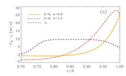
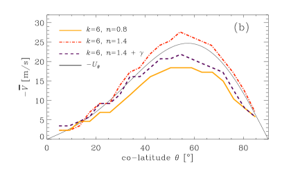
Figure 1: a) Radial profile of $U_{\theta}(r,57^{\circ})$ for different values of $n$. Dashed line: radial profile of $\gamma_{\theta}$, see eq. (1).  b) Corresponding tracking velocities, $\overline{V}$, for three cases: $\partial_{r}|U_{\theta}|>0$ (yellow/continuous) and $\partial_{r}|U_{\theta}|<0$ with (dashed) and without (red/dot-dashed) pumping. $\eta_{\rm T}=10^{12}\rm{cm}^{2}\!/s$ throughout.

To obtain a negative radial gradient of $|U_{\theta}|$ we preserve its general mathematical form (eq. (5) of GRBD), but choose the parameters of this ansatz as $k=6$ and $n=1.4$ which results in a negative $\partial_{r}|U_{\theta}|$ within a shallow surface-near layer of roughly 2% of the thickness of the convection zone (see Fig. 1a). It is worth mentioning that the stress-free boundary condition cannot be satisfied with a negative gradient. With this $U_{\theta}$ profile the velocities of the magnetic tracers turn out to be larger than the flow velocity (red/dot-dashed line in Fig. 1b). This result does not come unexpected since the field lines underneath the surface are pushed northwards by a flow faster than the surface one. By magnetic tension the field lines at the surface are then also accelerated. A snapshot of the magnetic field after two weeks of evolution is shown in Fig. 2a.

3 Additional transport mechanisms

Given that a negative $\partial_{r}|U_{\theta}|$ does not allow to reproduce the observations of decelerated magnetic tracer motion at the surface, one could be tempted to argue that the results of the ring diagram analysis could be incorrect. This conclusion, however, would be premature as our model is by no means complete. As mentioned in GRBD, studying axisymmetric, i.e., averaged fields requires the inclusion of the full mean electromotive force, from which only the turbulent diffusion term has so far been considered.

What about other constituents? Under anisotropic conditions, turbulence acts like a mean advective motion, called turbulent magnetic pumping and is described by a vector $\boldsymbol{\gamma}$. In the northern hemisphere, its $\theta$-component is found to be positive, i.e., equatorwards whereas its radial component is mainly negative (downwards), see [Käpylä et al. 2006a]. Being helical, convective turbulence in the rotating Sun exhibits also an $\alpha$-effect which together with differential rotation in the uppermost 35Mm of the convection zone (the so called near-surface shear layer) may well enable a turbulent dynamo of the $\alpha\Omega$ type. As $\partial_{r}\Omega<0$ there and $\alpha$ is expected to be positive in the northern hemisphere, the dynamo wave should, according to the Parker-Yoshimura rule, propagate equatorwards, contrary to the MC. This scenario is difficult to study as it requires establishing a full nonlinear mean-field dynamo model of the surface shear layer. Turbulent pumping, in contrast, can easily be introduced as an additive contribution to the MC.

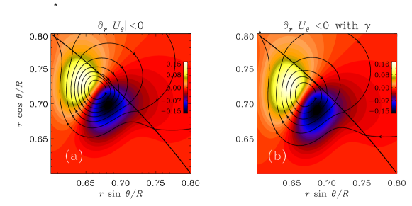
Figure 2: Magnetic field lines and $r$ component (color coded) after two weeks propagation, $\eta_{\rm T}=10^{12}\rm{cm}^{2}\!/s$. Velocity profile as in Fig. 1, red curve. a) without, b) with pumping, $\gamma_{0\theta}=10\,\rm{m}/\rm{s}$, see eq.(1)

.

We do so employing profiles for $\boldsymbol{\gamma}$ adapted from [Guerrero & de Gouveia Dal Pino (2008)] (hereafter GDP08):

$$\gamma_{\theta} = \gamma_{0\theta}\left[1+{\rm erf}\!\left(\frac{r-0.74}{0.035}\right)\right] \left[1-{\rm erf}\!\left(\frac{r-0.995}{0.05}\right)\right]\cos\theta\sin^{4}\theta,\quad\quad\quad\quad$$ (1)

$$\gamma_{r} = \,- \gamma_{0r}\left[1+{\rm erf}\!\left(\frac{r-0.7}{0.015}\right)\;\>\right] \left[1-{\rm erf}\!\left(\frac{r-0.975}{0.1}\right)\right]\!\!\left[\exp\!\left(\frac{r-0.715}{0.25}\right)^{2}\!\!\!\cos\theta+1\right]\!.$$

Similar to GDP08, we set $\gamma_{0r}$ and $\gamma_{0\theta}$ such that the maximum of $\gamma_{\theta}$ is 2.5 times larger than that of $\gamma_{r}$. The radial profile of $\gamma_{\theta}$, which is the more relevant component for this study, is shown with a broken line in Fig. 1a. From direct numerical simulations (DNS) [Käpylä et al. 2006a] have estimated that the maximum $\gamma_{\theta}$ should be $\approx 2.5$m/s. According to eq. (1) its value at the surface would then be $1.11$m/s. Given that the surface amplitude of $|U_{\theta}|\approx 25$m/s, this small value cannot significantly modify the results found in the previous section. Hence we have increased $\gamma_{0\theta}$ progressively and found that an MFT speed profile that roughly coincides with that of the flow speed is obtained with $\gamma_{0\theta}=5\rm{m/s}$ (i.e., $2.2$m/s at the surface or $\approx 10$% of the flow speed). For larger values of $\gamma_{0\theta}$ the MFT speed is smaller than the flow speed. In Fig. 1b we show the result obtained with the extraordinarily high value $\gamma_{0\theta}=10$m/s (see broken lines). Note that the latitudinal profile of $\gamma_{\theta}$ (eq. (1)) peaks at 63^∘ while the flow profile does at 57^∘. This is interesting because the resulting profile of the MFT speed peaks at a different latitude than the flow, just as it is obtained in observations (see fig. 10 of [Ulrich (2010), Ulrich, 2010]). Fig. 2 compares the morphology of the magnetic field from the simulation with pumping (b) to that without (a). Note that the magnetic field is transported further to the north in the case without magnetic pumping

Negative gradients $\partial_{r}|U_{\theta}|$ at the solar surface, as suggested by helioseismological ring-diagram analyses, result in MFT speeds higher than the plasma flow speed. By enhancing our flux transport model with turbulent magnetic pumping, we tried to reconcile the helioseismological results with the actually oberserved lower MFT speeds. However, high amplitudes of the pumping velocity not supported by DNS are needed. We have to conclude that either: (i) the negative gradient of $|U_{\theta}|$, suggested by ring-diagram analysis, if real, should be smaller than considered here, (ii) the pumping velocities from DNS are unrealistically low, which cannot be excluded because the setup in [Käpylä et al. 2006a] differs from the solar conditions, or (iii) the inclusion of the $\alpha$ effect in the flux transport model, enabling a dynamo process in the Sun’s surface shear layer, is crucial. For the latter, we have to think of a short-wavelength dynamo wave traveling equatorwards. Magnetic quenching would cause a corresponding $\theta$ modulation of $\alpha$, $\boldsymbol{\gamma}$ and $\eta_{\rm T}$ whereas the mean Lorentz force would modulate $U_{\theta}$ and $\Omega$. Here, quenching of $\eta_{\rm T}$ is perhaps most promising as the value of $\eta_{\rm T}$ “decides”to what degree the field is frozen in the fluid. Acknowledgment: We thank A. Muñoz-Jaramillo for pointing out the negative radial gradient of $|U_{\theta}|$ in the ring-diagram analysis and A. Kosovichev for his valuable comments.

References

- [Gonzáles Hernández et al.(2006)] Gonzáles Hernández, I., Komm, R., Hill, F., Howe, R., Corbard, T., Haber, D., 2006, ApJ, 638, 576
- [Guerrero et al. (2011)] Guerrero, G., Rheinhardt, M., Brandenburg, A., Dikpati M., 2011, MNRAS Letters, in press, (arXiv:1107.4801)
- [Guerrero & de Gouveia Dal Pino (2008)] Guerrero, G., de Gouveia Dal Pino, E. M., 2008, A&A, 485, 267
- [Hathaway & Rightmire (2010)] Hathaway, D. H., Rightmire, L., 2010, Science, 327, 1350
- [Käpylä et al. 2006a] Käpylä, P. J., Korpi, M. J., Ossendrijver, M., Stix, M., 2006a, A&A, 455, 401
- [Komm et al. (1993)] Komm, R. W., Howard, R. F., Harvey, J. W., 1993, Solar Physics, 147, 207
- [Ulrich (2010)] Ulrich, R. K., 2010, ApJ, 725, 658
- [Zhao et al. (2011)] Zhao, J., Couvidat, S., Bogart, R. S., Parchevsky, K. V., Birch, A. C., Duvall, T. L., Beck, J. G., Kosovichev, A. G., Scherrer, P. H., 2011, Solar Physics, pp 163–+