Monopoles, magnetricity and the stray field from spin ice

Abstract

An analysis is presented of the behaviour of muons in the low-temperature state in spin ice. It is shown in detail how the behavior observed in some previous muon experiments on spin ice in a weak transverse field may result from the macroscopic stray field of magnetized spin ice. A model is presented which allows these macroscopic field effects to be simulated and the results agree with experiment. The persistent spin dynamics at low temperature originate from the sample and could be a muon-induced implantation effect that is operative in out-of-equilibrium systems with long relaxation times.

Spin ice harris ; gingras ; jaubert2011 is the name given to compounds such as Dy₂Ti₂O₇ in which the magnetic Dy ions ($\mu\approx 10\mu_{\rm B}$) sit on a pyrochlore lattice (composed of corner-sharing tetrahedra) and are constrained by easy-axis anisotropy only to point in or out of each tetrahedron. The long-ranged dipolar interactions are almost perfectly screened at low temperatures hertog ; isakov so that the low-energy properties are essentially identical to an effective frustrated nearest-neighbour model equivalent to Pauling’s model for proton disorder in water ice pauling . The effective exchange energy in this dipolar Ising magnet is minimized if the moments on each tetrahedron satisfy the ice rules, namely that two spins point in and two spins point out harris . This results in a state whose large degeneracy is quantitatively consistent with the measured thermodynamic properties ramirez . Very recently it was realised that the natural excitations ryzhkin of spin ice can be described as magnetic monopoles castelnovo2008 : flipping a moment breaks the ice rules in two neighbouring tetrahedra (one tetrahedron has moments arranged three-out, one-in; its neighbor has one-out, three-in) and these states are positive and negative monopoles. Further flips allow these monopoles individually to hop through the lattice. This deconfined monopole picture is an economical description of the low-temperature behavior of spin ice, as one has moved from considering a concentrated collection of localised dipolar spins to a more dilute array of itinerant particles interacting Coulombically, a so-called magnetic Coulomb liquid castelnovo2008 .

The number of monopoles in spin ice can be estimated within the framework of Debye-Hückel (DH) theory castelnovo , see Fig. 1(a), and at very low temperatures the monopoles are very sparse indeed. It has been argued bramwell ; giblin that spin ice should conduct magnetic charge (“magnetricity”) in an analogous manner to an electrolyte and that Onsager’s theory onsager of the Wien effect should apply to spin ice. In this context, it is useful to consider the key lengthscales: the lattice spacing $a\approx 10$ Å (so that the distance from the centre of one tetrahedron to the centre of its neighbour is $r_{\rm d}=\sqrt{3}a/4\approx 4.4$ Å, and the monopole charge is $Q=2\mu/r_{\rm d}=4.50\mu_{\rm B}$Å^-1), the Bjerrum length $\ell_{\rm T}=\mu_{0}Q^{2}/(8\pi k_{\rm B}T)$ (the distance below which monopoles are bound by the Coulomb interaction), the field length $\ell_{\rm B}=k_{\rm B}T/QB$ (the lengthscale above which drift of monopoles in a field is discernable), the mean minimum distance between monopoles $\ell_{\rm m}$ (related to $n_{\rm f}$, the number density of free monopoles) and the Debye length $\ell_{\rm D}=(k_{\rm B}T/2\mu_{0}Q^{2}n_{\rm f})^{1/2}$ (the distance above which monopole charge density is screened) giblin . The temperature dependences of these lengthscales are plotted in Fig. 1(b).

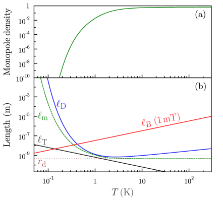
Figure 1: (a) The monopole density (in units of monopoles per tetrahedron) within the framework of Debye-Hückel theory castelnovo . (b) The key lengthscales in spin ice.

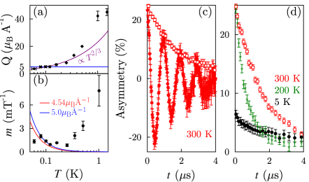
Figure 2: (a) The extracted monopole charge $Q$ from the data in Ref. bramwell, showing the plateau close to $Q=5\mu_{\rm B}$Å^-1, close to the theoretical value 4.54 $\mu_{\rm B}$Å^-1 castelnovo2008 . The low-$T$ data roughly follow a $T^{2/3}$ dependence. (b) The same data transformed to values of $m={1\over\lambda(0)}{{\rm d}\lambda(B)\over{\rm d}B}$ in order to test the expected $m\propto Q^{3}/T^{2}$ behavior, showing only limited agreement. (c,d) Data replotted from the study of Ref. lago, . (c) 300 K, filled points for a TF of 7.5 mT, open symbols for a longitudinal field of 5 mT (which was almost identical to zero-field data, but a small longitudinal field was used to quench any relaxation due to nuclear spins). (d) Measurements in a longitudinal field of 5 mT. Note the reduction in initial asymmetry in the 5 K data due to the largely static spin ice state.

One of the most ingenious experimental demonstrations of monopoles came from the muon-spin rotation ($\mu$SR) study of Bramwell et al. bramwell in which Dy₂Ti₂O₇ was subjected to a weak transverse field (TF). At very low temperature (in a regime such that $\ell_{\rm D}\gg\ell_{\rm B}\gtrsim\ell_{\rm T}$) it was argued that the relaxation rate of the muon precession signal $\lambda(B)$ in a magnetic field $B$ could be interpreted in terms of a fluctuation rate due to monopoles. By analogy with Onsager’s theory onsager , it was argued that one would expect $\lambda(B)/\lambda(0)\approx 1+\frac{b}{2}+\cdots$ where $b=\ell_{\rm T}/\ell_{\rm B}=\mu_{0}Q^{3}B/8\pi k_{\rm B}^{2}T^{2}$. This allows one to measure the field dependence of the relaxation rate and then infer the monopole charge $Q$. Bramwell et al. measured an exponentially damped precession signal, interpreting the form of the damping in terms of magnetic fluctuations resulting from monopoles. The analysis involved no free parameters and gave a value in very close agreement with the theoretical value $Q=4.50\mu_{\rm B}$Å^-1 castelnovo2008 [see Fig. 2(a)]. One prediction of this method is that the experimentally measured quantity $m={1\over\lambda(0)}{{\rm d}\lambda(B)\over{\rm d}B}=b/2B\propto T^{-2}$. As shown in Fig. 2(b), which replots the data of Ref. bramwell, , $m\propto T^{-2}$ only holds for a small subset of the data over a very limited range of $T$. Also, $Q\propto m^{1/3}T^{2/3}$ and it is seen in Fig. 2(a) that most of the temperature dependence in the low-temperature behavior of $Q$ is accounted for by the $T^{2/3}$ factor (present by definition), so that the closeness of the agreement with theory may not be so compelling as it first appears. Moreover because the measured $m(T)$ data [Fig. 2(b)] are found to fall on cooling down to $\sim 0.3$ K, below which they are approximately constant, a limited intersection with the hypothesized $m\propto T^{-2}$ curve is not unexpected even if the model is inapplicable.

Furthermore, despite the elegance of the theoretical approach, a surprising feature of these results was that any signal in a weak TF could be observed at all. An earlier $\mu$SR study using longitudinal-field decoupling lago had shown that the field at the muon site was around 0.5 T, so that a 2 mT field (the maximum field used in Ref. bramwell, ) would not be expected to lead to a precession signal. Some data from Ref. lago, are reproduced in Fig. 2(c,d). The relaxation of the precession signal in a TF at 300 K is the same as that observed in zero field [Fig. 2(c)]. That relaxation rate increases dramatically as the sample is cooled (following an activated behavior governed by transitions to/from the first excited state doublet of the crystal field lago ). At low $T$ [the 5 K data are shown in Fig. 2(d)] the relaxation is so fast that one can only measure the slower relaxation of the remaining “$\frac{1}{3}$-tail” (due to the component of the muon polarization parallel to the local field). These results are consistent with a largely static spin ice state.

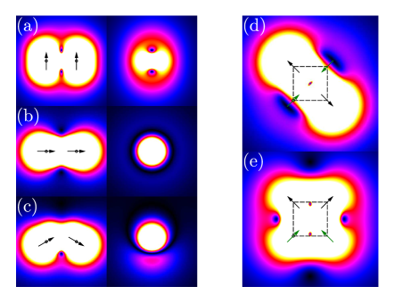
Figure 3: (Color online.) Distribution of $B_{\mu}$ in the vicinity of (a-c) two spins at positions $(\pm a,0,0)$, showing the field in the $y=0$ (left) and $x=0$ (right) planes, and (d-e) four spins on the corners of a tetrahedron (inscribed in a cube of side length $d$, centred at the origin), satisfying the ice rules. (d) $B_{\mu}$ is shown in the plane $z=0.44d$ with the spins at $z=d/2$ ($z=-d/2$) colored black (green). (e) $B_{\mu}$ in the plane $x=0$. The areas with the darkest colors have the smallest $B_{\mu}$.

To be sensitive to a weak TF, the field $B_{\mu}$ at the muon site needs to be very low. The hope that there might be some special site of field cancellation is not borne out by calculations, and the reason for this can be understood from the following considerations. First, it is found that the distribution of the magnitude of $B_{\mu}$ over the unit cell volume assuming various ordered arrangements of spins falls to zero for zero $B_{\mu}$ sjb , so that if present such zeros are extremely isolated and are unlikely to be obtained by chance. Even taking just two spins [say at positions $(\pm a,0,0)$] then the field zeros occupy either isolated points [e.g. if the moments $\parallel z$, then two zeros are found at $(0,0,\pm a/\sqrt{2})$, Fig. 3(a)] or in circles [e.g. if the moments are along $(\cos\alpha,0,\pm\sin\alpha)$, there is a circle of zeros in the $yz$ plane, centred at $(0,0,\frac{3}{2}\tan\alpha)$ with radius $\sqrt{2+\frac{9}{4}\tan^{2}\alpha}$, Fig. 3(b,c)]. For spins on the corners of a tetrahedron satisfying the spin ice rules only isolated zeros are found [see Fig. 3(d,e)]. Crucially their positions do not share the symmetry of the tetrahedron but depend on the particular spin ice configuration. Since muon sites depend on the electrostatic potential and reflect the crystal symmetry, then even if a particular muon sits at a site of field cancellation, many others will sit at crystallographically equivalent sites in which the field is far from zero. In a real crystal of Dy₂Ti₂O₇, containing many tetrahedra, the field from neighbouring tetrahedra (the spins on which can exist in many different configurations) will produce additional contributions which will displace or remove the zeros. In fact, the typical $B_{\mu}\sim(\mu_{0}/4\pi)\mu/r_{\rm d}^{3}\sim 0.1$ T, the same order as found in the earlier $\mu$SR experiment lago . This conclusion is in agreement with other recent calculations dunsiger ; castelnew . Thus it is surprising that applying a TF of $\sim 10^{-3}$ T in the experiment of Ref. bramwell, can have had any effect at all. Moreover, the recent experiment of Ref. dunsiger, provides evidence that no such precession signal is in fact observable when Dy₂Ti₂O₇ is mounted on GaAs and the experiment is repeated (so that muons missing the sample form muonium and do not contribute to the observed TF signal). However, the nature of the signal observed in Ref. bramwell, (with the sample mounted on silver), which seemingly produces a reasonable estimate of $Q$, has remained unaddressed.

I argue that the most likely resolution of this conundrum is that the TF muon signal which was observed originates from outside the sample (as suspected by Ref. dunsiger, ), and furthermore the particular pattern produced by a static, macroscopic exterior dipolar field produces a muon signal that could be misinterpreted as a dynamic signal. Exterior fields are well known to result from magnetized ferromagnets but are much more unusual in systems with no long range order. A macroscopic exterior field directly due to monopoles is unlikely because $\ell_{\rm D}\ll$sample size (unless $T<0.2\,$K, but even here $n_{\rm f}$ is likely to be larger than predicted by DH theory and strongly out of equilibrium bramwell2011 , keeping $\ell_{\rm D}$ small) but it is more likely due to the spin ice magnetization. When this exterior field distribution is “sampled” by muons implanted in the silver sample holder over the area close to the sample shown in Fig. 4(a), simulations show that the resulting relaxation function [Fig. 4(b)] mimics the exponentially relaxing signal reported in Ref. bramwell, .

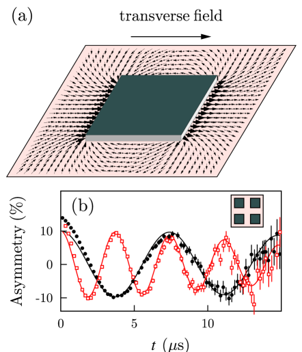
Figure 4: (a) The exterior field in the plane of the silver plate due to a sample magnetized horizontally and placed on top of the plate, evaluated from a closed analytic expression. The applied field adds to this exterior field. (b) The corresponding muon precession signal evaluated for the geometry shown in the inset, together with the 100 mK data from Ref. bramwell, . For this geometry, both $\chi$ and the ratio of sample (grey) to sample holder (pink) were fitted to the 2 mT data (red open squares). The fitted geometry is shown to scale and $\chi=0.45$. The 1 mT line was then evaluated with no further parameter adjustment (data black filled circles).

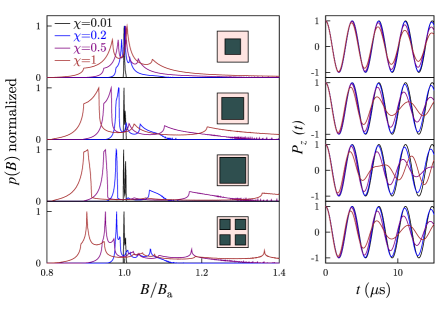
Figure 5: The field distribution $p(B)$ for the muon averaged over the silver plate for a variety of sample geometries (shown in the insets) and values of $\chi$. Also shown are the corresponding simulated muon precession signals $P_{z}(t)$ for a field of 2 mT.

The simulation of this phenomenon proceeds as follows: In an applied magnetic field ${\bf B}_{\rm a}=\mu_{0}{\bf H}_{\rm a}$, the field inside and outside the sample is given by ${\bf H}({\bf r})=(1-\chi{\cal N}({\bf r})){\bf H}_{\rm a}$, where $\chi$ is the magnetic susceptibility and ${\cal N}({\bf r})$ is a symmetrical 3$\times$3 demagnetization tensor that depends on position ${\bf r}$ even outside the sample, which is of particular interest to us. This expression is valid under the assumption that the magnetization inside the sample is uniform. For a sample with a cuboidal shape an analytical closed form for ${\cal N}({\bf r})$ can be used joseph . With the initial polarization along $\hat{\bf n}$, the resulting time-dependence of the muon polarization can be evaluated using

$$P_{\hat{\bf n}}(t)={1\over A}\int{\rm d}{\bf r}\left({B_{\parallel}({\bf r})^{2}\over B({\bf r})^{2}}+{B_{\perp}({\bf r})^{2}\over B({\bf r})^{2}}\cos\gamma_{\mu}B({\bf r})t\right),$$ (1)

where the integral is over the area $A$ of the silver sample holder surrounding the sample in which muons are implanted. Outside the sample ${\bf B}=\mu_{0}{\bf H}$ and we have $B_{\parallel}({\bf r})={\bf B}\cdot\hat{\bf n}$ and $B_{\perp}({\bf r})=|{\bf B}({\bf r})-B_{\parallel}({\bf r})\hat{\bf n}|$. Thus if ${\bf B}_{\rm a}$ is along $\hat{\bf x}$ and one is measuring $P_{z}(t)$, then $B_{\parallel}({\bf r})=\chi B_{\rm a}{\cal N}_{13}({\bf r})$ and $B_{\perp}({\bf r})=B_{\rm a}\sqrt{(1-\chi{\cal N}_{11}({\bf r}))^{2}+\chi^{2}{\cal N}_{21}({\bf r})^{2}}$. The only parameters in this model are (i) the value of $\chi$ and (ii) the geometry of the experiment, specifically the size of the region outside the sample sampled by the muons. Unless $\chi\gg 1$, the oscillatory component of $P_{z}(t)$ dominates and this can be written $\int p(B)\cos\gamma_{\mu}Bt\,{\rm d}B$ where the function $p(B)$ is plotted in Fig. 5 for various geometries and values of $\chi$, together with the corresponding $P_{z}(t)$. The distribution $p(B)$ contains van Hove singularities of the macroscopic field distribution and broadens with increasing $\chi$. It depends on the precise shapes and arrangements of crystallites on the sample holder, with large density far from $B_{\rm a}$ due to regions close to the crystallites. The fit to data in Fig. 4(b) is quite reasonable (and corresponds to $\chi=0.45$ and the geometry shown in the inset), though fits with other geometries are possible. This value of $\chi$ at 0.1 K is larger than observed in zero-field cooled magnetization data snyder2004 , but falls short of the equilibrium susceptibility of spin ice $\chi=\sqrt{3}\pi\ell_{\rm T}/r_{\rm d}\approx 80$ ryzhkin2011 , showing that the magnetization is still slowly developing matsuhira2011 (and this is indeed a manifestation of the Wien effect bramwell ). A single muon measurement at a particular $B_{\rm a}$ and $T$ is performed of a timescale of $\sim 1$ hour, so that the effect of slow dynamics (the monopole hop rate $\sim 10^{3}$ s^-1) can become important. Were larger values of $\chi$ to be obtained in experiment, the simulations in Fig. 5 show that the TF precession signals should become strongly distorted by the very strong stray fields, an effect that can be looked for in future experiments.

The very fast initial relaxation in the data bramwell , not fitted in our formalism [see first 1 $\mu$s in Fig. 4(b)] is due to spin dynamics from muons stopped in the sample lago , superimposed on the weak TF signal. The motion of a monopole is accompanied by the reversal of a Dy spin, resulting in a change $\Delta B_{\mu}$ of up to $(2\mu_{0}/4\pi)2\mu/r^{3}$, where $r$ is the distance from the Dy moment to the muon. Within a radius of $\approx 50$ Å around the muon there are $\sim 10^{4}$ Dy ions, each of which can produce a $\Delta B_{\mu}$ from tenths to tens of mT. Thus even though during the $\mu$SR measurement timescale ($\approx 20$ $\mu$s) most monopoles appear static (and the muon experiences a largely frozen field distribution as discussed above), because the monopole hop rate is only $\sim 10^{3}$ s^-1jaubert ; snyder2004 , the muon is coupled sufficiently strongly to such a large number of Dy ions that even an occasional monopole hop will be enough to contribute to measurable relaxation in the $\frac{1}{3}$-tail. The inferred fluctuation rate of $\sim 10^{6}$ s^-1 lago from this relaxation is thus entirely consistent with this picture. Moreover the muon relaxation rate would be expected to track the underlying monople dynamics (thus the plateau observed in the relaxation time $\tau$ from a.c. susceptibility snyder2004 is found also in $\mu$SR lago , albeit at a scaled rate). Below 1 K however, $n_{\rm f}$ drops dramatically [see Fig. 1(a)] and $\tau$ diverges, while the muon relaxation rate stays approximately constant lago ; dunsiger ; jmmm , an example of the phenomenon of persistent spin dynamics observed in many frustrated systems mcclarty . To understand this effect in Dy₂Ti₂O₇ it is worth remembering that the muon itself brings substantial kinetic energy at implantation. In the final stage of its thermalization, it loses energy from several tens of keV via charge exchange cycles whereby an electron successively adds to and is stripped from the muon cox99 . It is conceivable that this process can nucleate monopoles in the sample (the system is unable to rapidly transport heat away and is susceptible to thermal runaway quenches ; runaway ), and when this muon-induced concentration exceeds the equilibrium concentration, the monopole-induced muon relaxation rate will settle at a fixed value. Such an explanation could have wider applicability in other frustrated magnets.

I am particularly grateful to the following for helpful and enjoyable discussions: Steve Bramwell, Claudio Castelnovo, Sean Giblin, Michel Gingras, Peter Holdsworth, Jorge Lago, Tom Lancaster, Roderich Moessner and Jorge Quintanilla. This work is supported by the EPSRC, UK.

References

- (1) M. J. Harris, S. T. Bramwell, D. F. McMorrow, T. Zeiske and K. W. Godfrey, Phys. Rev. Lett.79, 2554 (1997).
- (2) S. T. Bramwell and M. J. P. Gingras, Science 294, 1495 (2001).
- (3) L. D. C. Jaubert and P. C. W. Holdsworth, J. Phys.: Condens. Matter 23, 164222, (2011)
- (4) B. C. den Hertog and M. J. P. Gingras, Phys. Rev. Lett. 84, 3430 (2000); B. C. den Hertog and M. J. P. Gingras, Can. J. Phys. 79, 1339 (2001).
- (5) S. V. Isakov, R. Moessner and S. L. Sondhi, Phys. Rev. Lett. 95, 217201 (2005).
- (6) L. Pauling, J. Am. Chem. Soc. 57, 2680 (1935).
- (7) A. P. Ramirez, A. Hayashi, R. J. Cava, R. Siddharthan, and B. S. Shastry, Nature (London) 399, 333 (1999).
- (8) I. A. Ryzhkin, JETP 101, 481 (2005).
- (9) C. Castelnovo, R. Moessner, and S. L. Sondhi, Nature (London) 451, 42 (2008).
- (10) C. Castelnovo, R. Moessner, and S. L. Sondhi, Phys. Rev. B 84, 144435 (2011).
- (11) S. T. Bramwell, S. R. Giblin, S. Calder, R. Aldus, D. Prabhakaran, and T. Fennell, Nature (London) 461, 956 (2009).
- (12) S. R. Giblin, S. T. Bramwell, P. C. W. Holdsworth, D. Prabhakaran, and I. Terry, Nature Physics 7, 252 (2011).
- (13) L. Onsager, J. Chem. Phys. 2, 599 (1934).
- (14) J. Lago, S. J. Blundell, and C. Baines, J. Phys.: Condens. Matter 19, 326210, (2007)
- (15) S. J. Blundell, Phil. Trans. R. Soc. Lond. A357, 2923 (1999); S. J. Blundell, Physica B 404, 581 (2009).
- (16) S. R. Dunsiger et al. Phys. Rev. Lett. 107, 207207 (2011)
- (17) G. Sala, C. Castelnovo, R. Moesnner, S. L. Sondhi, T. Kitagawa, R. Higashinaka, and Y. Maeno, unpublished.
- (18) S. T. Bramwell, J. Phys.: Condens. Matter 23, 112201, (2011)
- (19) R. I. Joseph and E. Schloemann, J. Appl. Phys. 36, 1579 (1965).
- (20) J. Snyder, B. G. Ueland, J. S. Slusky, H. Karunadasa, R. J. Cava, and P. Schiffer, Phys. Rev. B 69, 064414 (2004).
- (21) I. A. Ryzhkin and M. I. Ryzhkin, JETP 93, 384 (2011).
- (22) K. Matsuhira, C. Paulsen, E. Lhotel, C. Sekine, Z. Hiroi and S. Takagi, J. Phys. Soc. Jpn. 80, 123711 (2011).
- (23) L. D. C. Jaubert and P. C. W. Holdsworth, Nature Physics 5, 258 (2009).
- (24) M. J. Harris, S. T. Bramwell, T. Zeiske, D. F. McMorrow, and P. J. C. King J. Mag. Mag. Mat. 177, 757 (1998)
- (25) P. A. McClarty, J. N. Cosman, A. G. Del Maestro, and M. J. P. Gingras, J. Phys. Condens. Matter 23, 164216 (2011).
- (26) S. F. J. Cox, Rep. Prog. Phys. 72, 116501 (2009).
- (27) C. Castelnovo, R. Moessner, and S. L. Sondhi, Phys. Rev. Lett. 104, 107201 (2010).
- (28) D. Slobinsky, C. Castelnovo, R. A. Borzi, A. S. Gibbs, A. P. Mackenzie, R. Moessner, and S. A. Grigera, Phys. Rev. Lett. 105, 267205 (2010).