Interest Rates and Information Geometry

Abstract

The space of probability distributions on a given sample space possesses natural geometric properties. For example, in the case of a smooth parametric family of probability distributions on the real line, the parameter space has a Riemannian structure induced by the embedding of the family into the Hilbert space of square-integrable functions, and is characterised by the Fisher-Rao metric. In the nonparametric case the relevant geometry is determined by the spherical distance function of Bhattacharyya. In the context of term structure modelling, we show that minus the derivative of the discount function with respect to the maturity date gives rise to a probability density. This follows as a consequence of the positivity of interest rates. Therefore, by mapping the density functions associated with a given family of term structures to Hilbert space, the resulting metrical geometry can be used to analyse the relationship of yield curves to one another. We show that the general arbitrage-free yield curve dynamics can be represented as a process taking values in the convex space of smooth density functions on the positive real line. It follows that the theory of interest rate dynamics can be represented by a class of processes in Hilbert space. We also derive the dynamics for the central moments associated with the distribution determined by the yield curve. (26 June 2000)

Keywords: Interest rate models, Heath-Jarrow-Morton framework,
principal moments analysis, differential geometry and statistics

1 Introduction

The theory of interest rates has gone through two major developments in recent decades. Following initial investigations by Merton (1973) and others, the first decisive advance culminated in the work of Vasicek (1977) who was able to give a fairly general characterisation of the arbitrage-free dynamics of a family of discount bonds, indexed by their maturity. The well-known model that bears his name appears as an exact solution obtained with specialising assumptions. In the wake of Vasicek’s work were a number of other specific interest rate models, of varying degrees of usefulness and tractability, including, for example, the CIR model (Cox et al. 1985) and its generalisations. The next significant line of development, following the general martingale characterisation of arbitrage-free asset pricing by Harrison $\&$ Kreps (1979) and Harrison $\&$ Pliska (1981), was instigated with the recognition by Ho $\&$ Lee (1986) that the initial term structure might be specified essentially arbitrarily, a feature that has important practical implications. This insight was incorporated into the HJM framework (Heath et al. 1992), which constituted a major advance in the subject, providing a general model-independent basis for the analysis of interest rate dynamics and the pricing of interest rate derivatives.

Since then there have been numerous further developments. These include, for example, the infinite dimensional or ‘string-type’ models of Kennedy (1994), Santa-Clara $\&$ Sornett (1997) and others, the positive interest rate models of Flesaker $\&$ Hughston (1996), the potential approach of Rogers (1997), the so-called market models (Brace et al. 1996, 1997; Jamshidian 1997), and the geometric analysis of the space of yield curves undertaken by Björk $\&$ Svensson (1999).

Nevertheless, no criterion has emerged, based on the extensive econometric evidence available, that allows in a rational way for the identification of a clearly preferred class of models. On these grounds it makes sense to try to cast the general interest rate framework into a new form, with the idea that certain models might thus become recognisable as more natural on mathematical and economic grounds.

With this end in mind, the purpose of the present article is to propose a novel application of information geometry to interest rate theory. The main results are (i) the construction of a geometric measure for how ‘different’ two term structures are from one another; (ii) a characterisation of the evolutionary trajectory of the term structure as a measure-valued process; (iii) the derivation of dynamics for the principal moments of the term structure; and (iv) a reformulation of arbitrage-free interest rate dynamics in terms of a class of processes on Hilbert space.

The paper is organised as follows. In §2 we review the basic idea of information geometry and its role in estimation theory. The geometry of the normal distribution is considered in detail as an illustration. In §3 a remarkable characterisation of the discount function in terms of an abstract probability density function is introduced in Proposition 1. This allows us to apply information geometric techniques to determine the deviation between different term structures within a given model. In this connection, in §4 we consider a class of flat rate models as examples.

The material of the first four sections of the paper is essentially static, i.e., set in the present, whereas in §5 we investigate the dynamics of the density function that generates the term structure. This is carried out in such a way that the resulting dynamics is manifestly arbitrage-free. Our key result here is formula (5.47), in which we establish that the dynamics of the term structure can be characterised as a measure-valued process. This idea is developed further in Proposition 2.

In §6 we introduce an analogue of the classical principal components analysis for yield curves, and in Propositions 3 and 4 we derive formulae for the evolution of the first two moments of the term structure density process. Then, making use of the information geometry developed earlier, in §7 we map the dynamics developed in §5 to Hilbert space. Our main result here is Proposition 5, which shows how this can be achieved.

2 Information geometry

Because some of the mathematical techniques we employ here may not be familiar to those working in finance, it will be appropriate to begin with a few background remarks. It has long been known (see, e.g., Amari 1985; Kass 1989; Murray $\&$ Rice 1993) that a useful approach to statistical inference is to regard a parametric model as a differentiable manifold equipped with a metric. The recognition that a parametric family of probability distributions has a natural geometry associated with it arose in the work of Mahalanobis (1936), Bhattacharyya (1943) and Rao (1945) over half of a century ago.

Suppose, for example, that $X$ is a continuous random variable taking values on the real line ${\bf R}^{1}$, and that $\mathchar 28954\relax(x)$ is a density function for $X$. Because $\mathchar 28954\relax(x)$ is nonnegative and has integral unity, it follows that the square-root likelihood function

$$\mathchar 28952\relax(x)=\sqrt{\mathchar 28954\relax(x)}$$ (2.1)

exists for all $x$, and satisfies the normalisation condition

$$\int_{-\infty}^{\infty}(\mathchar 28952\relax(x))^{2}{\rm d}x=1.$$ (2.2)

We see that $\mathchar 28952\relax(x)$ can be regarded as a unit vector in the Hilbert space ${\cal H}=L^{2}({\bf R}^{1})$. Now let $\mathchar 28954\relax_{1}(x),\mathchar 28954\relax_{2}(x)$ denote a pair of density functions on ${\bf R}^{1}$, and $\mathchar 28952\relax_{1}(x),\mathchar 28952\relax_{2}(x)$ the corresponding Hilbert space elements. Then the inner product

$$\cos\mathchar 28958\relax=\int_{-\infty}^{\infty}\mathchar 28952\relax_{1}(x)\mathchar 28952\relax_{2}(x){\rm d}x$$ (2.3)

defines an angle $\mathchar 28958\relax$ which can be interpreted as the distance between the two probability distributions. More precisely, if we write ${\cal S}$ for the unit sphere in ${\cal H}$, then $\mathchar 28958\relax$ is the spherical distance between the points on ${\cal S}$ determined by the vectors $\mathchar 28952\relax_{1}(x)$ and $\mathchar 28952\relax_{2}(x)$. The maximum possible distance, corresponding to nonoverlapping densities, is given by $\mathchar 28958\relax=\mathchar 28953\relax/2$. This follows from the fact that $\mathchar 28952\relax_{1}(x)$ and $\mathchar 28952\relax_{2}(x)$ are nonnegative functions, and thus define points on the positive orthant of ${\cal S}$. We remark that an alternative way of expressing (2.3) is

$$\cos\mathchar 28958\relax=1-\frac{1}{2}\int_{-\infty}^{\infty}(\left(\mathchar 28952\relax_{1}(x)-\mathchar 28952\relax_{2}(x)\right)^{2}{\rm d}x,$$ (2.4)

which makes it apparent that the angle $\mathchar 28958\relax$ measures the extent to which the two distributions are distinct.

The spherical distance of Bhattacharyya introduced above is applicable in a nonparametric context. In the case of a parametric family of probability distributions we can develop matters further. Let us write $\mathchar 28954\relax(x,\mathchar 28946\relax)$ for the parameterised density function. Here $\mathchar 28946\relax$ stands for a set of parameters $\mathchar 28946\relax^{i}$ $(i=1,\cdots,r)$. By varying $\mathchar 28946\relax$ we obtain an $r$-dimensional submanifold ${\cal M}$ in ${\cal S}$ determined by the unit vectors $\mathchar 28952\relax(x,\mathchar 28946\relax)\in{\cal H}$. The parameters $\mathchar 28946\relax^{i}$ are local coordinates for ${\cal M}$.

The key point that we require in the following (cf. Dawid 1977) is that the spherical geometry of ${\cal S}$ induces a Riemannian geometry on ${\cal M}$, for which the metric tensor $g_{ij}(\mathchar 28946\relax)$ is given, in local coordinates, by

$$g_{ij}(\mathchar 28946\relax)=\int_{-\infty}^{\infty}\frac{\partial\mathchar 28952\relax(x,\mathchar 28946\relax)}{\partial\mathchar 28946\relax^{i}}\frac{\partial\mathchar 28952\relax(x,\mathchar 28946\relax)}{\partial\mathchar 28946\relax^{j}}{\rm d}x.$$ (2.5)

By use of definition (2.1), we see that an alternative expression for $g_{ij}(\mathchar 28946\relax)$ is

$$g_{ij}(\mathchar 28946\relax)=\frac{1}{4}\int_{-\infty}^{\infty}\mathchar 28954\relax(x,\mathchar 28946\relax)\frac{\partial\ln\mathchar 28954\relax(x,\mathchar 28946\relax)}{\partial\mathchar 28946\relax^{i}}\frac{\partial\ln\mathchar 28954\relax(x,\mathchar 28946\relax)}{\partial\mathchar 28946\relax^{j}}{\rm d}x,$$ (2.6)

which shows (cf. Brody $\&$ Hughston 1998) that the metric $g_{ij}$ is, apart from the factor of $\frac{1}{4}$, the Fisher information matrix, i.e., the covariance matrix of the parametric gradient of the log-likelihood function (Fisher 1921). We refer to $g_{ij}(\mathchar 28946\relax)$ as the Fisher-Rao metric on the statistical model ${\cal M}$.

The significance of the Fisher-Rao metric in estimation theory is well known. Suppose that $\mathchar 28956\relax(\mathchar 28946\relax)$ is some given function of the parameters, and that the random variable $T$ represented by the function $T(x)$ on ${\bf R}^{1}$ is an unbiased estimator for $\mathchar 28956\relax(\mathchar 28946\relax)$ in the sense that

$$\int_{-\infty}^{\infty}\mathchar 28954\relax(x,\mathchar 28946\relax)T(x){\rm d}x=\mathchar 28956\relax(\mathchar 28946\relax).$$ (2.7)

The variance of the estimator $T$ is defined, as usual, by

$${\rm Var}[T]=\int_{-\infty}^{\infty}\mathchar 28954\relax(x,\mathchar 28946\relax)(T(x)-\mathchar 28956\relax(\mathchar 28946\relax))^{2}{\rm d}x.$$ (2.8)

Then a set of fundamental bounds on ${\rm Var}[T]$, independent of the choice of the estimator $T(x)$, can be obtained by applying the operator $\sum_{i}\mathchar 28939\relax^{i}\partial_{i}$ to (2.7), letting $\mathchar 28939\relax^{i}$ be arbitrary. By use of (2.1) and the Schwartz inequality for $L^{2}({\bf R}^{1})$, we obtain

$$g_{ij}{\rm Var}[T]\geq\frac{1}{4}\frac{\partial\mathchar 28956\relax}{\partial\mathchar 28946\relax^{i}}\frac{\partial\mathchar 28956\relax}{\partial\mathchar 28946\relax^{j}}.$$ (2.9)

This matrix inequality is interpreted as saying that if we subtract the right side from the left, the result is nonnegative definite. It follows that if the random variables $\Theta^{i}$ $(i=1,\cdots,r)$ are unbiased estimators for the parameters $\mathchar 28946\relax^{i}$, satisfying

$$\int_{-\infty}^{\infty}\mathchar 28954\relax(x,\mathchar 28946\relax)\Theta^{i}(x){\rm d}x=\mathchar 28946\relax^{i},$$ (2.10)

then the covariance matrix of the estimators is bounded by the inverse Fisher information matrix:

$${\rm Cov}[\Theta^{i},\Theta^{j}]\geq\frac{1}{4}g^{ij}.$$ (2.11)

The Riemannian metric (2.5) introduced above can be used to define a distance measure between two distributions belonging to a given parametric family. This measure is invariant in the sense that it is unaffected by a reparameterisation of the distributions. The distance is calculated by integrating the infinitesimal line element ${\rm d}s$ along the geodesic connecting the two points in the statistical manifold ${\cal M}$, where

$${\rm d}s^{2}=\sum_{i,j}g_{ij}{\rm d}\mathchar 28946\relax^{i}{\rm d}\mathchar 28946\relax^{j}.$$ (2.12)

The geodesics with respect to a given metric $g_{ij}$ are the solutions of the differential equation

$$\frac{{\rm d}^{2}\mathchar 28946\relax^{i}}{{\rm d}u^{2}}+\Gamma^{i}_{jk}\frac{{\rm d}\mathchar 28946\relax^{j}}{{\rm d}u}\frac{{\rm d}\mathchar 28946\relax^{k}}{{\rm d}u}=0$$ (2.13)

for the curve $\mathchar 28946\relax^{i}(u)$ in ${\cal M}$, subject to the given boundary conditions at the two end points. Here, we have written

$$\Gamma^{i}_{jk}=\frac{1}{2}g^{il}\left(\partial_{j}g_{kl}+\partial_{k}g_{jl}-\partial_{l}g_{jk}\right),$$ (2.14)

where $\partial_{i}=\partial/\partial\mathchar 28946\relax^{i}$, and the inverse metric $g^{ij}$, also appearing in (2.11), satisfies $g^{ij}g_{jk}=\mathchar 28942\relax^{i}_{k}$, where $\mathchar 28942\relax^{i}_{k}$ is the Kronecker delta. Note that in equations (2.13) and (2.14) above, and elsewhere henceforth in this article, we employ the standard Einstein summation convention on repeated indices.

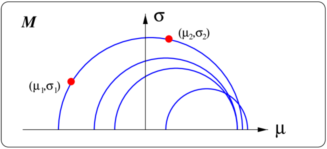
Figure 1: Geodesic curves for normal distributions. The statistical manifold ${\cal M}$ in this case is the upper half plane parameterised by $\mathchar 28950\relax$ and $\mathchar 28955\relax$. We have $-\infty<\mathchar 28950\relax<\infty$ and $0<\mathchar 28955\relax<\infty$. The shortest path joining the two normal distributions ${\cal N}(\mathchar 28950\relax_{1},\mathchar 28955\relax_{1})$ and ${\cal N}(\mathchar 28950\relax_{2},\mathchar 28955\relax_{2})$ is given by the unique semi-circular arc through the given two points and centred on the boundary line $\mathchar 28955\relax=0$.

Let us consider, as an explicit example, the manifold ${\cal M}$ corresponding to the normal distributions ${\cal N}(\mathchar 28950\relax,\mathchar 28955\relax)$ on ${\bf R}^{1}$, with mean $\mathchar 28950\relax$ and standard deviation $\mathchar 28955\relax$. For the parameterised density function we have

$$\mathchar 28954\relax(x,\mathchar 28950\relax,\mathchar 28955\relax)=\frac{1}{\sqrt{2\mathchar 28953\relax}\mathchar 28955\relax}\exp\left(-\frac{(x-\mathchar 28950\relax)^{2}}{2\mathchar 28955\relax^{2}}\right).$$ (2.15)

A straightforward computation, making use of (2.6), gives

$${\rm d}s^{2}=\frac{1}{\mathchar 28955\relax^{2}}({\rm d}\mathchar 28950\relax^{2}+2{\rm d}\mathchar 28955\relax^{2})$$ (2.16)

for the line element, which is defined on the upper half-plane $-\infty<\mathchar 28950\relax<\infty$, $0<\mathchar 28955\relax<\infty$. The resulting Riemannian geometry is that of hyperbolic space, which is a homogeneous manifold with constant negative curvature. The geometry of this space has been studied extensively, and has many intriguing properties. For the distance function in the case of a pair of normal distributions ${\cal N}(\mathchar 28950\relax_{1},\mathchar 28955\relax_{1})$, ${\cal N}(\mathchar 28950\relax_{2},\mathchar 28955\relax_{2})$ we obtain

$$D(\mathchar 28954\relax_{1},\mathchar 28954\relax_{2})=\frac{1}{\sqrt{2}}\log\frac{1+\mathchar 28942\relax_{1,2}}{1-\mathchar 28942\relax_{1,2}},$$ (2.17)

where the function $\mathchar 28942\relax_{1,2}$, defined by

$$\mathchar 28942\relax_{1,2}=\sqrt{\frac{(\mathchar 28950\relax_{2}-\mathchar 28950\relax_{1})^{2}+2(\mathchar 28955\relax_{2}-\mathchar 28955\relax_{1})^{2}}{(\mathchar 28950\relax_{2}-\mathchar 28950\relax_{1})^{2}+2(\mathchar 28955\relax_{2}+\mathchar 28955\relax_{1})^{2}}},$$ (2.18)

lies between 0 and 1. The geodesics, in particular, are given in general by semi-circular arcs centred on the boundary line $\mathchar 28955\relax=0$ (this line itself is not part of the manifold ${\cal M}$). An exceptional situation arises when $\mathchar 28950\relax_{1}=\mathchar 28950\relax_{2}$, for which the geodesic is a straight line given by constant $\mathchar 28950\relax$, and we have

$$D(\mathchar 28954\relax_{1},\mathchar 28954\relax_{2})=\frac{1}{\sqrt{2}}\left|\log\frac{\mathchar 28955\relax_{1}}{\mathchar 28955\relax_{2}}\right|.$$ (2.19)

We refer the reader to Burbea (1986), where metric and distance computations have been carried out explicitly for other families of distributions.

3 Discount bond densities

Our goal now is to make use of the analysis presented in the previous section to construct a natural metric on the space of yield curves. In doing so we shall take advantage of a remarkable ‘probabilistic’ characterisation of discount bonds, which we here proceed to describe.

Let $t=0$ denote the present, and $P_{0T}$ a smooth family of discount bonds, where $T$ is the maturity date $(0\leq T<\infty)$. For positive interest we require

$$0<P_{0T}\leq 1,\ \ \ \frac{\partial}{\partial T}P_{0T}<0,$$ (3.20)

and we assume that $P_{0T}\rightarrow 0$ as $T$ goes to infinity. A term structure that satisfies these conditions will be said to be ‘admissible’. These conditions can, in fact, be relaxed slightly: $P_{0T}$ need not be strictly smooth, nor strictly decreasing; but for most of the present discussion we shall stick with the assumptions indicated.

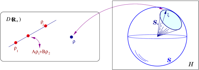
Figure 2: The system of admissible term structures. A smooth positive interest term structure can be regarded as a point in ${\cal D}({\bf R}_{+}^{1})$, the convex space consisting of smooth density functions on ${\bf R}_{+}^{1}$. The points of ${\cal D}({\bf R}_{+}^{1})$ are in one-to-one correspondence with rays lying in the positive orthant ${\cal S}_{+}$ of the unit sphere ${\cal S}$ in the Hilbert space ${\cal H}=L^{2}({\bf R}_{+}^{1})$.

The interesting point that arises here, of which we shall make extensive use in the discussions that follow, is that the discount function $P_{0T}$ can be viewed as a complementary probability distribution. In other words, we think of the maturity date as an abstract random variable $X$, and for its distribution we write

$${\bf P}[X<T]=1-P_{0T}.$$ (3.21)

It should be clear that this can be done if and only if the positive interest rate conditions given in (3.20) hold. As a consequence we are able to embody the positive interest property in a fundamental way in the structure of the theory. Indeed, this basic economic property is essential if we wish to treat the yield curve consistently and naturally as a kind of mathematical object in its own right. Now let us introduce the function $\mathchar 28954\relax(T)$ defined by

$$\mathchar 28954\relax(T)=-\frac{\partial}{\partial T}P_{0T}.$$ (3.22)

Clearly, we have $\mathchar 28954\relax(T)>0$ and

$$\int_{0}^{\infty}\mathchar 28954\relax(T){\rm d}T=1,$$ (3.23)

from which we infer that $\mathchar 28954\relax(T)$ can be consistently viewed as a probability density function. It follows from the defining equation (3.22) that the term structure density $\mathchar 28954\relax(T)$ is the product of the instantaneous forward rate and the discount function itself. Now clearly if $\mathchar 28954\relax_{1}(T)$ and $\mathchar 28954\relax_{2}(T)$ are admissible term structure densities, and if $A$ and $B$ are nonnegative constants satisfying $A+B=1$, then $A\mathchar 28954\relax_{1}(T)+B\mathchar 28954\relax_{2}(T)$ is also an admissible term structure density. Putting these ingredients together, we see that the term structure of interest rates can be given the following general characterisation.

Proposition 1

The system of admissible term structures is isomorphic to the convex space ${\cal D}({\bf R}_{+}^{1})$ of smooth density functions on the positive real line.

At first glance it may seem odd to think of the discount function in this manner. However, it gives us the advantage of being able to apply the tools of information geometry in an unexpected way, as we indicate in what follows.

In particular, there is a one-to-one map from the space ${\cal D}({\bf R}_{+}^{1})$ of such term structure densities to the positive orthant ${\cal S}_{+}$ of the unit sphere ${\cal S}$ in the Hilbert space ${\cal H}$, as indicated in Figure 2. Therefore, given two yield curves we can calculate the distance between them. This can be carried out either in a nonparametric sense, by use of the Bhattacharyya spherical distance, or in a parametric sense, by use of the Fisher-Rao distance. In the former case first we calculate the corresponding term structure densities $\mathchar 28954\relax_{1}(T)$ and $\mathchar 28954\relax_{2}(T)$. These are then mapped to ${\cal S}_{+}$ by taking the square-roots, and their distance $\mathchar 28958\relax(\mathchar 28954\relax_{1},\mathchar 28954\relax_{2})$ is given by

$$\mathchar 28958\relax(\mathchar 28954\relax_{1},\mathchar 28954\relax_{2})=\cos^{-1}\int_{0}^{\infty}\sqrt{\mathchar 28954\relax_{1}(T)\mathchar 28954\relax_{2}(T)}{\rm d}T.$$ (3.24)

In the parametric case we regard the given parametric family of yield curves as defining a statistical model ${\cal M}\subset{\cal S}_{+}$, and the distance between the two yield curves within the given family is then defined by the Fisher-Rao metric.

4 Flat term structures

To provide some illustrations of the principles set forth in the previous section we consider here properties of yield curves for which the term structure is flat. Such yield curves, which are of various types, are on the whole too simple for use in practical modelling. Nevertheless, they are of interest as examples, because many of the relevant computations can be carried out explicitly.

In this connection we begin by introducing a representation of the discount function as a Laplace transform

$$P_{0T}=\int_{0}^{\infty}e^{-rT}\mathchar 28960\relax(r){\rm d}r$$ (4.25)

for some function $\mathchar 28960\relax(r)$. Thus we think of the discount function $P_{0T}$ as being given by a weighted superposition of elementary discount functions, each of the form $e^{-rT}$ for some value of $r$. Taking the limit $T\rightarrow 0$, we find that $\mathchar 28960\relax(r)$ must satisfy $\int_{0}^{\infty}\mathchar 28960\relax(r){\rm d}r=1$. In general the inverse Laplace transform $\mathchar 28960\relax(r)$ need not be positive. However, if we restrict our consideration to nonnegative functions, then $\mathchar 28960\relax(r)$ can be interpreted as a density function, and by various choices of $\mathchar 28960\relax(r)$ we are led to some interesting candidates for term structures.

First we consider the case where $\mathchar 28960\relax(r)$ is a Dirac $\mathchar 28942\relax$-function concentrated at a point, that is, $\mathchar 28960\relax(r)=\mathchar 28942\relax(r-R)$. A direct substitution gives $P_{0T}=\exp(-RT)$, corresponding to a ‘flat’ term structure with a continuously compounded rate $R$ for each value of the maturity date $T$. If the density function $\mathchar 28960\relax(r)$ is given by an exponential distribution $\mathchar 28960\relax(r)=\mathchar 28956\relax\exp(-\mathchar 28956\relax r)$, with parameter $\mathchar 28956\relax$, then one sees that $\mathchar 28956\relax$ must have dimensions of time, and a short calculation gives $P_{0T}=\mathchar 28956\relax/(\mathchar 28956\relax+T)$, which also corresponds to a flat term structure, in this case with a simple percentage yield of $\mathchar 28956\relax^{-1}$ for all maturities. We see that the characteristic time-scale $\mathchar 28956\relax$ allows us to define an interest rate $R=\mathchar 28956\relax^{-1}$, which turns out to be the characteristic interest rate of the resulting structure, and we can write $P_{0T}=1/(1+RT)$ for the discount function.

We note that flatness is not a completely unambiguous notion, because having a uniform continuously compounded yield for all maturities is not the same thing as having a uniform simple yield for all maturities. Both define plausible albeit quite distinct systems of discount bonds. This example illustrates how by superposing term structures of the elementary form $\exp(-RT)$ for various maturities, we can obtain other reasonable looking and well behaved term structures. We mention one more example, which contains the previous two examples as special cases. Consider the standard gamma distribution, with parameters $\mathchar 28948\relax$ and $\mathchar 28949\relax$, defined for nonnegative values of $r$ by the density function

$$\mathchar 28960\relax(r)=\frac{1}{\Gamma(\mathchar 28948\relax)}\mathchar 28949\relax^{\mathchar 28948\relax}r^{\mathchar 28948\relax-1}\exp(-\mathchar 28949\relax r).$$ (4.26)

In this case, we can verify that the resulting system of discount bonds is given by

$$P_{0T}=\left(\frac{\mathchar 28949\relax}{\mathchar 28949\relax+T}\right)^{\mathchar 28948\relax},$$ (4.27)

which assumes a more recognisable form if we set $\mathchar 28949\relax=\mathchar 28948\relax\mathchar 28956\relax$, where $\mathchar 28956\relax$ again defines a characteristic time scale, and $\mathchar 28948\relax$ is a dimensionless number. Then we have

$$P_{0T}=\left(1+\frac{RT}{\mathchar 28948\relax}\right)^{-\mathchar 28948\relax},$$ (4.28)

where $R=\mathchar 28956\relax^{-1}$. The system of discount bonds arising here can also be interpreted as a flat term structure, in this case with a constant annualised rate of interest $R$ assuming compounding at the frequency $\mathchar 28948\relax$ over the life of each bond ($\mathchar 28948\relax$ need not be an integer). It is not difficult to check that for $\mathchar 28948\relax=1$ this reduces to the case of a flat rate on the basis of a simple yield, whereas in the limit $\mathchar 28948\relax\rightarrow\infty$ we recover the case of a flat rate on the basis of continuous compounding.

Now we shall apply the ideas of statistical geometry to make comparisons between various term structures of the form (4.28). For density function $\mathchar 28954\relax(T)=-\partial_{T}P_{0T}$ in this case we obtain

$$\mathchar 28954\relax(T,R)=R\left(1+\frac{RT}{\mathchar 28948\relax}\right)^{-(\mathchar 28948\relax+1)}.$$ (4.29)

Here we find it convenient to label the density function by the flat rate $R$. Note that in the limit $\mathchar 28948\relax\rightarrow\infty$ we have $\mathchar 28954\relax(T,R)\rightarrow Re^{-RT}$. First consider the nonparametric separation between different term structures in this model via spherical distance of Bhattacharyya given in formula (3.24), where in the present example we write $\mathchar 28954\relax_{i}(T)=\mathchar 28954\relax(T,R_{i})$ for $i=1,2$. A direct integration leads to the expression

$$\mathchar 28958\relax(\mathchar 28954\relax_{1},\mathchar 28954\relax_{2})=\cos^{-1}\left(\frac{\sqrt{R_{1}R_{2}}}{R_{1}-R_{2}}\log\frac{R_{1}}{R_{2}}\right)$$ (4.30)

for the distance when $\mathchar 28948\relax=1$, whereas in the limit $\mathchar 28948\relax\rightarrow\infty$ (continuous compounding) we have

$$\mathchar 28958\relax(\mathchar 28954\relax_{1},\mathchar 28954\relax_{2})=\cos^{-1}\left(\frac{2\sqrt{R_{1}R_{2}}}{R_{1}+R_{2}}\right).$$ (4.31)

It is interesting to observe that the bracketed term in (4.31) is given by the ratio of the geometric and arithmetic means of the two rates.

Alternatively, we can view (4.29) as a parametric family of distributions, parameterised by the flat rate $R$. Then it is natural to consider the Fisher-Rao distance between the two term structures characterised by $R_{1}$ and $R_{2}$. A straightforward calculation then leads to a simple distance formula given by

$$D(R_{1},R_{2})=\sqrt{\frac{\mathchar 28948\relax}{\mathchar 28948\relax+2}}\log\frac{R_{2}}{R_{1}},$$ (4.32)

where we have assumed $R_{2}\geq R_{1}$.

5 Interest rate dynamics

The formalism we have developed so far is essentially a static one, set in the present. Now we turn to the problem of developing a dynamical theory of interest rates. The idea is that, at each instant of time, the yield curve is characterised by a term structure density according to the scheme described in the previous sections. Then, as time passes, the density function evolves randomly. As a consequence we obtain a measure-valued process. In particular, we obtain a process on ${\cal D}({\bf R}_{+}^{1})$. Our goal in this section is to determine a set of conditions on this process necessary and sufficient to ensure that the resulting interest rate dynamics will be arbitrage-free.

We shall assume the reader is familiar with the general theory of interest rate dynamics as laid out, for example, in Carverhill (1994), Rogers (1994), Hughston (1996), Baxter (1997), Musiela $\&$ Rutkowski (1997), Brody (2000) or Hunt $\&$ Kennedy (2000). For the general discount bond dynamics, let us write

$${\rm d}P_{tT}=\mathchar 28950\relax_{tT}{\rm d}t+\Sigma_{tT}\cdot{\rm d}W_{t},$$ (5.33)

where $\mathchar 28950\relax_{tT}$ and $\Sigma_{tT}$ are the absolute drift and absolute volatility processes, respectively, for a bond with maturity $T$. Here, $W_{t}$ is a vector Brownian motion, and $\Sigma_{tT}$ is a vector process, and there is an inner product implied between $\Sigma_{tT}$ and ${\rm d}W_{t}$, signified by a dot. We need not specify the dimensionality of the Brownian motion, which might be infinite, and indeed in some respects the infinite dimensional setting is the most natural one. In fact, it suffices for our purposes merely to assume that $P_{tT}$ is a one-parameter family of continuous semi-martingales on the given probability space, with respect to the given filtration. However, for simplicity of exposition we shall stick to the case where the relevant stochastic basis is generated by a multidimensional Brownian motion. Here, as in Flesaker $\&$ Hughston (1997a,b), we regard the discount bond dynamics as the natural starting position, rather than, say, the instantaneous forward rate dynamics (Heath et al. 1992), which we need not consider here directly. We shall assume nevertheless, as in the HJM framework, that the processes $\mathchar 28950\relax_{tT}$ and $\Sigma_{tT}$ are both smooth in the variable $T$, and that sufficiently strong technical conditions are in place to ensure that the instantaneous forward rate processes are semimartingales.

In order to extend the analysis of the previous section it is convenient to introduce what is sometimes conveniently referred to as the ‘Musiela parameterisation’, given by

$$B_{tx}=P_{t,t+x},$$ (5.34)

where $T=t+x$ represents the maturity date of the bond, and hence $x$ is the time left until maturity. Thus $B_{tx}$ is the value at time $t$ of a discount bond that has $x$ years left to mature. This choice of parameterisation has already been shown to be useful in the geometric analysis of interest rates (Björk $\&$ Svensson 1999, Björk $\&$ Christensen 1999, Björk $\&$ Gombani 1999, Björk 2000). We note that $B_{t0}=1$ for all $t$, and that $B_{tx}\rightarrow 0$ as $x\rightarrow\infty$. It follows that

$$\mathchar 28954\relax_{t}(x)=-\frac{\partial}{\partial x}B_{tx}$$ (5.35)

is a measure-valued process in the sense that, for each value of $t$ the random function $\mathchar 28954\relax_{t}(x)$ satisfies $\mathchar 28954\relax_{t}(x)>0$ and the normalisation condition

$$\int_{0}^{\infty}\mathchar 28954\relax_{t}(x){\rm d}x=1.$$ (5.36)

Here we have chosen the notation $\mathchar 28954\relax_{t}(x)$ that makes the $x$ dependence more prominent, to emphasise the fact that, for each value of $t$, and conditional on information given up to time $t$, $\mathchar 28954\relax_{t}(x)$ is a density function, though we might have written $\mathchar 28954\relax_{tx}$ instead. As a consequence $\mathchar 28954\relax_{t}(x)$ describes a process on ${\cal D}({\bf R}_{+}^{1})$. By consideration of (5.33) and (5.34) we deduce for the dynamics of $B_{tx}$ that

$${\rm d}B_{tx}=\left.{\rm d}P_{tT}\right|_{T=t+x}+\frac{\partial}{\partial x}B_{tx}{\rm d}t,$$ (5.37)

and thus, by use of (5.33), that

$${\rm d}B_{tx}=\left(\mathchar 28950\relax_{t,t+x}+\partial_{x}B_{tx}\right){\rm d}t+\Sigma_{t,t+x}\cdot{\rm d}W_{t},$$ (5.38)

where $\partial_{x}=\partial/\partial x$. Differentiating this expression with respect to $x$ and introducing the measure-valued process $\mathchar 28954\relax_{t}(x)$ according to formula (5.35) we therefore obtain

$${\rm d}\mathchar 28954\relax_{t}(x)=\left(-\partial_{x}\mathchar 28950\relax_{t,t+x}+\partial_{x}\mathchar 28954\relax_{t}(x)\right){\rm d}t-\partial_{x}\Sigma_{t,t+x}\cdot{\rm d}W_{t}.$$ (5.39)

A further simplification is then achieved by introducing the notation

$$\mathchar 28940\relax_{tx}=-\partial_{x}\mathchar 28950\relax_{t,t+x}$$ (5.40)

and

$$\mathchar 28961\relax_{tx}=-\partial_{x}\Sigma_{t,t+x},$$ (5.41)

which gives us

$${\rm d}\mathchar 28954\relax_{t}(x)=\left(\mathchar 28940\relax_{tx}+\partial_{x}\mathchar 28954\relax_{t}(x)\right){\rm d}t+\mathchar 28961\relax_{tx}\cdot{\rm d}W_{t}.$$ (5.42)

In the foregoing discussion we have not yet imposed the arbitrage-free condition. This is given by the drift constraint

$$\mathchar 28950\relax_{tT}=r_{t}P_{tT}+\Sigma_{tT}\cdot\mathchar 28949\relax_{t},$$ (5.43)

where $\mathchar 28949\relax_{t}$ is the process for the market price of risk. We note that $\mathchar 28949\relax_{t}$, like $\Sigma_{tT}$, is a vector process. However, $\mathchar 28949\relax_{t}$ does not depend on the maturity $T$. The absence of arbitrage ensures the existence of $\mathchar 28949\relax_{t}$. For our purposes we do not need to insist that the bond market is complete: all we require is the existence of a pricing kernel, or equivalently the existence of a self-financing ‘natural numeraire’ portfolio with value process $N_{t}$ such that $P_{tT}/N_{t}$ is a martingale for each value of $T$ (cf. Flesaker $\&$ Hughston 1997c). The numeraire process satisfies

$$\frac{{\rm d}N_{t}}{N_{t}}=(r_{t}+\mathchar 28949\relax_{t}^{2}){\rm d}t+\mathchar 28949\relax_{t}\cdot{\rm d}W_{t},$$ (5.44)

and the corresponding pricing kernel is given by $1/N_{t}$. As a consequence of the constraint (5.43) we then have

$$\mathchar 28950\relax_{t,t+x}=r_{t}B_{tx}+\Sigma_{t,t+x}\cdot\mathchar 28949\relax_{t},$$ (5.45)

and therefore, by differentiation of this expression with respect to $x$, we obtain

$$\mathchar 28940\relax_{tx}=r_{t}\mathchar 28954\relax_{t}(x)+\mathchar 28961\relax_{tx}\cdot\mathchar 28949\relax_{t}.$$ (5.46)

Inserting (5.46) in (5.42) we are thus able to express the dynamics of the density function $\mathchar 28954\relax_{t}(x)$ in the form

$${\rm d}\mathchar 28954\relax_{t}(x)=\left(r_{t}\mathchar 28954\relax_{t}(x)+\partial_{x}\mathchar 28954\relax_{t}(x)\right){\rm d}t+\mathchar 28961\relax_{tx}\cdot\left({\rm d}W_{t}+\mathchar 28949\relax_{t}{\rm d}t\right).$$ (5.47)

Before proceeding further, let us verify, as a consistency check, that the dynamics given by (5.47) preserves the normalisation condition on $\mathchar 28954\relax_{t}(x)$, given by (5.36). Integrating the right hand side of (5.47) with respect to $x$ and equating the drift and volatility terms separately to zero leads to the relations

$$r_{t}+\int_{0}^{\infty}\partial_{x}\mathchar 28954\relax_{t}(x){\rm d}x=0$$ (5.48)

and

$$\int_{0}^{\infty}\mathchar 28961\relax_{tx}{\rm d}x=0,$$ (5.49)

which must hold for all $t$. Condition (5.48) is satisfied because $\mathchar 28954\relax_{t}(x)\rightarrow 0$ as $x\rightarrow\infty$ and

$$\mathchar 28954\relax_{t}(0)=r_{t}.$$ (5.50)

Condition (5.49) is satisfied because, by definition, we have $\mathchar 28961\relax_{tx}=-\partial_{x}\Sigma_{t,t+x}$, and the absolute volatility $\Sigma_{t,t+x}$ vanishes both as $x\rightarrow 0$ (a maturing bond has a definite value and thus has no absolute volatility), and as $x\rightarrow\infty$ (a bond with infinite maturity has no value, and hence no absolute volatility).

Summing up matters so far, we see that in (5.47) we are able to cut the standard HJM arbitrage-free interest rate dynamics in the form of a measure-valued process $\mathchar 28954\relax_{t}(x)$ subject to the constraints (5.48) and (5.49). At first glance the role of the short rate $r_{t}$ in (5.47) seems anomalous, because it might appear that this has to be specified separately. However, by virtue of (5.50) we can incorporate $r_{t}$ directly into the dynamics of $\mathchar 28954\relax_{t}(x)$.

In fact, there is another way of expressing (5.47) which is very suggestive, and ties in naturally with the Hilbert space approach to dynamics introduced in §7. First we note that (5.48) can be rewritten in the form

$$r_{t}=-\int_{0}^{\infty}\mathchar 28954\relax_{t}(x)\partial_{x}\ln\mathchar 28954\relax_{t}(x){\rm d}x.$$ (5.51)

In other words, $r_{t}$ is minus the expectation of the gradient of the log-likelihood function. Here the expectation is taken with respect to $\mathchar 28954\relax_{t}(x)$ itself. Writing $E_{\mathchar 28954\relax}$ for this abstract expectation, we have

$${\rm d}\mathchar 28954\relax_{t}(x)=\mathchar 28954\relax_{t}(x)\left(\partial_{x}\ln\mathchar 28954\relax_{t}(x)-E_{\mathchar 28954\relax}[\partial_{x}\ln\mathchar 28954\relax_{t}(x)]\right){\rm d}t+\mathchar 28961\relax_{tx}\cdot{\rm d}W_{t}^{*},$$ (5.52)

where ${\rm d}W_{t}^{*}={\rm d}W_{t}+\mathchar 28949\relax_{t}{\rm d}t$. We note that $W_{t}^{*}$ has the interpretation of being a Brownian motion with respect to the risk-neutral measure associated with the given pricing kernel. In the risk-neutral measure, for which the term involving $\mathchar 28949\relax_{t}$ effectively disappears, the remaining drift for $\mathchar 28954\relax_{t}(x)$ is determined by the deviation of $\partial_{x}\ln\mathchar 28954\relax_{t}(x)$ from its abstract mean.

Let us now examine more closely the volatility term $\mathchar 28961\relax_{tx}$ appearing in (5.52), with a view to gaining a better understanding of the significance of the volatility constraint (5.49). Because $\mathchar 28954\relax_{t}(x)$ must remain positive for all values of $x$, the coefficient of ${\rm d}W_{t}^{*}$ in (5.52) must be of the form

$$\mathchar 28961\relax_{tx}=\mathchar 28954\relax_{t}(x)\mathchar 28955\relax_{tx}$$ (5.53)

for some bounded process $\mathchar 28955\relax_{tx}$, to ensure that $\mathchar 28961\relax_{tx}$ dies off appropriately for values of $x$ such that $\mathchar 28954\relax_{t}(x)$ approaches zero. As a consequence, we can write (5.47) in the quasi-lognormal form

$$\frac{{\rm d}\mathchar 28954\relax_{t}(x)}{\mathchar 28954\relax_{t}(x)}=(r_{t}+\partial_{x}\ln\mathchar 28954\relax_{t}(x)){\rm d}t+\mathchar 28955\relax_{tx}\cdot{\rm d}W_{t}^{*},$$ (5.54)

and for the constraint (5.49) we have

$$E_{\mathchar 28954\relax}[\mathchar 28955\relax_{tx}]=0,$$ (5.55)

which can be satisfied by writing

$$\mathchar 28955\relax_{tx}=\mathchar 28951\relax_{tx}-E_{\mathchar 28954\relax}[\mathchar 28951\relax_{tx}],$$ (5.56)

where $\mathchar 28951\relax_{tx}$ is an exogenously specifiable unconstrained process. Here, for any process $A_{tx}$ we define $E_{\mathchar 28954\relax}[A_{tx}]=\int_{0}^{\infty}\mathchar 28954\relax_{t}(x)A_{tx}{\rm d}x$. The results established above can then be summarised as follows.

Proposition 2

The general admissible term structure evolution based on the information set generated by a multidimensional Brownian motion $W_{t}$ is given by a measure-valued process $\mathchar 28954\relax_{t}(x)$ in ${\cal D}({\bf R}_{+}^{1})$ satisfying

$$\frac{{\rm d}\mathchar 28954\relax_{t}(x)}{\mathchar 28954\relax_{t}(x)} = \left(\partial_{x}\ln\mathchar 28954\relax_{t}(x)-E_{\mathchar 28954\relax}[\partial_{x}\ln\mathchar 28954\relax_{t}(x)]\right){\rm d}t$$ (5.57)

$$+\left(\mathchar 28951\relax_{tx}-E_{\mathchar 28954\relax}[\mathchar 28951\relax_{tx}]\right)\cdot\left({\rm d}W_{t}+\mathchar 28949\relax_{t}{\rm d}t\right),$$

where the processes $\mathchar 28949\relax_{t}$ and $\mathchar 28951\relax_{tx}$ are specified exogenously, along with the initial term structure density $\mathchar 28954\relax_{0}(x)$.

An advantage of the particular expression (5.57) given for the dynamics above is that the preservation of the normalisation condition on $\mathchar 28954\relax_{t}(x)$ is evident by inspection, because this is equivalent to the relation

$$E_{\mathchar 28954\relax}\left[\frac{{\rm d}\mathchar 28954\relax_{t}(x)}{\mathchar 28954\relax_{t}(x)}\right]=0.$$ (5.58)

An alternative expression for (5.57), which brings out more explicitly the nonlinearities in the dynamics, is given by

$${\rm d}\mathchar 28954\relax_{t}(x) = \left(\partial_{x}\mathchar 28954\relax_{t}(x)+\mathchar 28954\relax_{t}(0)\mathchar 28954\relax_{t}(x)\right){\rm d}t$$ (5.59)

$$+\mathchar 28954\relax_{t}(x)\left(\mathchar 28951\relax_{tx}-\int_{0}^{\infty}\mathchar 28954\relax_{t}(y)\mathchar 28951\relax_{ty}{\rm d}y\right)\cdot{\rm d}W^{*}_{t},$$

where ${\rm d}W^{*}_{t}={\rm d}W_{t}+\mathchar 28949\relax_{t}{\rm d}t$ as defined earlier.

6 Principal moment analysis

The characterisation of the yield curve as an abstract probability density enables us to develop a rigourous analogue of the classical ‘principal component’ analysis often used in the study of yield curve dynamics. To this end we let $\mathchar 28954\relax_{t}(x)=-\partial_{x}P_{t,t+x}$ be the density process associated with an admissible family of discount bond prices, and define the moment processes

$${\bar{x}}_{t}=\int_{0}^{\infty}x\mathchar 28954\relax_{t}(x){\rm d}x$$ (6.60)

and

$${\bar{x}}_{t}^{\prime(n)}=\int_{0}^{\infty}x^{n}\mathchar 28954\relax_{t}(x){\rm d}x$$ (6.61)

for $n\geq 2$, along with the central moment processes

$${\bar{x}}_{t}^{(n)}=\int_{0}^{\infty}(x-{\bar{x}}_{t})^{n}\mathchar 28954\relax_{t}(x){\rm d}x.$$ (6.62)

It is important to note that in some cases the relevant moments may not exist. For example, in the case of a continuously compounded flat yield curve given at $t=0$ by the density function $\mathchar 28954\relax_{0}(x)=R{\rm e}^{-Rx}$, we have ${\bar{x}}_{0}=R^{-1}$, ${\bar{x}}_{0}^{(2)}=R^{-2}$, ${\bar{x}}_{0}^{(3)}=3R^{-3}$, and ${\bar{x}}_{0}^{(4)}=9R^{-4}$ for the first four central moments. On the other hand, in the example of the simple flat term structure for which $\mathchar 28954\relax_{0}(x)=R/(1+Rx)^{2}$ we find that none of the moments exist, on account of the fatness of the tail of the distribution. In fact, for the flat rate term structures with compounding frequency $\mathchar 28948\relax$ the moments exist only up to order $\mathchar 28948\relax-1$.

The first four moments, if they exist, are the mean, variance, skewness and kurtosis of the distribution of the abstract random variable $X$ characterising the yield curve, and we refer to these (and other) moments as the ‘principal moments’ of the given term structure. At $t=0$ the mean ${\bar{x}}_{0}$ determines a characteristic time-scale associated with the given term structure, and its inverse $1/{\bar{x}}_{0}$ can be thought of as an associated characteristic yield. The difference ${\bar{x}}_{0}^{(2)}-({\bar{x}}_{0})^{2}$ then measures the departure of the given term structure from flatness on a continuously compounded basis. This is on account of the fact that in the case of an exponential distribution the variance is given by the square of the mean.

It is legitimate to conjecture that for some purposes the specification of, e.g., the first three or four moments will be sufficient to provide an accurate representation of the term structure. One way of implementing this idea is to introduce the entropy $S_{\mathchar 28954\relax}$ of the given distribution, defined by

$$S_{\mathchar 28954\relax}=-\int_{0}^{\infty}\mathchar 28954\relax(x)\ln\mathchar 28954\relax(x){\rm d}x.$$ (6.63)

Because $\mathchar 28954\relax(x)$ has dimensions of inverse time, $S_{\mathchar 28954\relax}$ is defined only up to an overall additive constant. Therefore, the difference of the entropies associated with two yield curves has an invariant significance.

For yield curve calibration we propose that $\mathchar 28954\relax(x)$ should be chosen such that $S_{\mathchar 28954\relax}$ is maximised subject to the constraints of the data available. For example, if we are given as data only the mean ${\bar{x}}_{0}$, then the maximum entropy term structure is $\mathchar 28954\relax_{0}(x)=Re^{-Rx}$, where $R=1/{\bar{x}}_{0}$.

It is also of great interest to study the dynamics of the principal characteristics in the case of a general admissible arbitrage-free term structure. We examine here, in particular, the mean and the variance processes. For this purpose we introduce a simplified notation $v_{t}={\bar{x}}_{t}^{(2)}$ for the variance process, i.e.,

$$v_{t}=\int_{0}^{\infty}x^{2}\mathchar 28954\relax_{t}(x){\rm d}x-({\bar{x}}_{t})^{2},$$ (6.64)

where the mean process ${\bar{x}}_{t}$ is given as in (6.60). We assume that both $\mathchar 28954\relax_{t}(x)$ and the discount bond volatility $\Sigma_{t,t+x}$ fall off to zero sufficiently rapidly to ensure that $\lim_{x\rightarrow\infty}x^{n}\mathchar 28954\relax_{t}(x)=0$ and $\lim_{x\rightarrow\infty}x^{n}\Sigma_{t,t+x}=0$ for $n=1,2$, and that the integrals $\int_{0}^{\infty}x^{n}\mathchar 28954\relax_{t}(x){\rm d}x$ and $\int_{0}^{\infty}x^{n-1}\Sigma_{t,t+x}{\rm d}x$ exist for $n=1,2$. A straightforward calculation then leads us to the following conclusion:

Proposition 3

The first principal moment ${\bar{x}}_{t}$ of an admissible, arbitrage-free term structure satisfies the dynamical law

$${\rm d}{\bar{x}}_{t}=(r_{t}{\bar{x}}_{t}-1){\rm d}t+{\bar{\Sigma}}_{t}\cdot{\rm d}W^{*}_{t},$$ (6.65)

where ${\bar{\Sigma}}_{t}=\int_{0}^{\infty}\Sigma_{t,t+x}{\rm d}x$.

Proof. Starting with (5.54) and (6.60) we have

$${\rm d}{\bar{x}}_{t} = \int_{0}^{\infty}x{\rm d}\mathchar 28954\relax_{t}(x){\rm d}x$$ (6.66)

$$= \left(r_{t}{\bar{x}}_{t}+\int_{0}^{\infty}x\partial_{x}\mathchar 28954\relax_{t}(x){\rm d}x\right){\rm d}t-\left(\int_{0}^{\infty}x\partial_{x}\Sigma_{t,t+x}{\rm d}x\right)\cdot{\rm d}W_{t}^{*}$$

by use of (5.41). Then, integrating by parts and using the assumed asymptotic behaviours for $\mathchar 28954\relax_{t}(x)$ and $\Sigma_{t,t+x}$, we obtain the desired result. $\diamondsuit$

We note that there is a critical level ${\bar{x}}_{t}^{*}$ for the first principal moment given by

$${\bar{x}}_{t}^{*}=\frac{1}{r_{t}}(1-\mathchar 28949\relax_{t}\cdot{\bar{\Sigma}}_{t}).$$ (6.67)

When ${\bar{x}}_{t}>{\bar{x}}_{t}^{*}$ the drift of ${\bar{x}}_{t}$ is positive, and the drift increases further as ${\bar{x}}$ increases. On the other hand, when ${\bar{x}}_{t}<{\bar{x}}_{t}^{*}$, the drift of ${\bar{x}}_{t}$ is negative, and the drift decreases further as ${\bar{x}}_{t}$ decreases. For the variance process, we have:

Proposition 4

The second principal moment $v_{t}$ of an admissible, arbitrage-free term structure satisfies the dynamical law

$${\rm d}v_{t}=\left(r_{t}(v_{t}-{\bar{x}}_{t}^{2})-{\bar{\Sigma}}_{t}^{2}\right){\rm d}t+2\left({\bar{\Sigma}}_{t}^{(1)}-{\bar{x}}_{t}{\bar{\Sigma}}_{t}\right)\cdot{\rm d}W_{t}^{*},$$ (6.68)

where ${\bar{\Sigma}}_{t}^{(1)}=\int_{0}^{\infty}x\Sigma_{t,t+x}{\rm d}x$.

Proof. Starting with formula (6.64) for $v_{t}$ we have

$${\rm d}v_{t}=\int_{0}^{\infty}x^{2}{\rm d}\mathchar 28954\relax_{t}(x){\rm d}x-{\rm d}({\bar{x}}_{t}^{2}).$$ (6.69)

For the first term we obtain

$$\int_{0}^{\infty}x^{2}\mathchar 28954\relax_{t}(x){\rm d}x = \left(r_{t}\int_{0}^{\infty}x^{2}\mathchar 28954\relax_{t}(x){\rm d}x+\int_{0}^{\infty}x^{2}\partial_{x}\mathchar 28954\relax_{t}(x){\rm d}x\right){\rm d}t$$ (6.70)

$$-\left(\int_{0}^{\infty}x^{2}\partial_{x}\Sigma_{t,t+x}\right)\cdot{\rm d}W_{t}^{*},$$

where we have used (5.41) and (5.54). As a consequence of the assumed asymptotic behaviour of $\mathchar 28954\relax_{t}(x)$ and $\Sigma_{t,t+x}$, this becomes

$$\int_{0}^{\infty}x^{2}\mathchar 28954\relax_{t}(x){\rm d}x=\left(r_{t}{\bar{x}}_{t}^{\prime(2)}-2{\bar{x}}_{t}\right){\rm d}t+2{\bar{\Sigma}}_{t}^{(1)}\cdot{\rm d}W_{t}^{*},$$ (6.71)

after an integration by parts. For the second term in (6.69) we have

$${\rm d}({\bar{x}}_{t}^{2})=2{\bar{x}}_{t}{\rm d}{\bar{x}}_{t}+({\rm d}{\bar{x}}_{t})^{2}$$ (6.72)

by Ito’s lemma, and thus

$${\rm d}({\bar{x}}_{t}^{2})=\left(2r_{t}{\bar{x}}_{t}^{2}-2{\bar{x}}_{t}+\Sigma_{t}^{2}\right){\rm d}t+2{\bar{x}}_{t}{\bar{\Sigma}}_{t}\cdot{\rm d}W_{t}^{*}$$ (6.73)

by use of Proposition 3. Combining (6.71) and (6.73), and using the definition (6.64) we obtain (6.68). $\diamondsuit$

In this case we recall that the difference $v_{t}-{\bar{x}}_{t}^{2}$ acts as a simple measure of the extent to which the distribution deviates from the ‘flat’ term structure. As a consequence we see that the effect of the dynamics here is that the second principal moment of the term structure tends to increase, i.e., has a positive drift, providing $v_{t}-{\bar{x}}_{t}^{2}$ is already above the level given by

$$v_{t}-{\bar{x}}_{t}^{2}=\frac{1}{r_{t}}\left({\bar{\Sigma}}_{t}^{2}-2\mathchar 28949\relax_{t}\cdot({\bar{\Sigma}}_{t}^{(1)}-{\bar{x}}_{t}{\bar{\Sigma}}_{t})\right).$$ (6.74)

7 Hilbert space dynamics for term structures

Now that we have examined some of the advantages of expressing the arbitrage-free interest rate term structure dynamics as a randomly evolving density function, let us consider how we transform to the Hilbert space representation for density functions considered in §2. Denote by $\mathchar 28952\relax_{tx}$ the process for the square-root likelihood function, defined by

$$\mathchar 28954\relax_{t}(x)=\mathchar 28952\relax_{tx}^{2}.$$ (7.75)

It follows then, by Ito’s lemma, that

$${\rm d}\mathchar 28954\relax_{t}(x)=2\mathchar 28952\relax_{tx}{\rm d}\mathchar 28952\relax_{tx}+({\rm d}\mathchar 28952\relax_{tx})^{2},$$ (7.76)

and hence $({\rm d}\mathchar 28954\relax_{t}(x))^{2}=4\mathchar 28952\relax_{tx}^{2}({\rm d}\mathchar 28952\relax_{tx})^{2}$. By rearranging (7.76) we thus obtain

$${\rm d}\mathchar 28952\relax_{tx}=\frac{1}{2\mathchar 28952\relax_{tx}}{\rm d}\mathchar 28954\relax_{t}(x)-\frac{1}{8\mathchar 28952\relax_{tx}^{3}}({\rm d}\mathchar 28954\relax_{t}(x))^{2}$$ (7.77)

for the dynamics of the process $\mathchar 28952\relax_{tx}$, and hence

$${\rm d}\mathchar 28952\relax_{tx}=\left(\partial_{x}\mathchar 28952\relax_{tx}+\frac{1}{2}r_{t}\mathchar 28952\relax_{tx}-\frac{1}{8\mathchar 28952\relax_{tx}^{3}}\mathchar 28961\relax_{tx}^{2}\right){\rm d}t+\frac{1}{2\mathchar 28952\relax_{tx}}\mathchar 28961\relax_{tx}\cdot{\rm d}W_{t}^{*},$$ (7.78)

where $\mathchar 28961\relax^{2}_{tx}=\mathchar 28961\relax_{tx}\cdot\mathchar 28961\relax_{tx}$. Now suppose we define $\mathchar 28955\relax_{tx}$ by the quotient

$$\mathchar 28955\relax_{tx}=\frac{\mathchar 28961\relax_{tx}}{\mathchar 28952\relax_{tx}^{2}},$$ (7.79)

as before, and set $\mathchar 28955\relax_{tx}^{2}=\mathchar 28955\relax_{tx}\cdot\mathchar 28955\relax_{tx}$. Then the process for the square-root density $\mathchar 28952\relax_{tx}$ can be written in the form

$${\rm d}\mathchar 28952\relax_{tx}=\left(\partial_{x}\mathchar 28952\relax_{tx}+\mbox{$\textstyle\frac{1}{2}$}r_{t}\mathchar 28952\relax_{tx}-\mbox{$\textstyle\frac{1}{8}$}\mathchar 28952\relax_{tx}\mathchar 28955\relax_{tx}^{2}\right){\rm d}t+\mbox{$\textstyle\frac{1}{2}$}\mathchar 28952\relax_{tx}\mathchar 28955\relax_{tx}\cdot{\rm d}W_{t}^{*}.$$ (7.80)

We recall that the volatility process $\mathchar 28955\relax_{tx}$ arising again in this connection, which is given more explicitly by the ratio

$$\mathchar 28955\relax_{tx}=\frac{\partial_{x}\Sigma_{t,t+x}}{\partial_{x}B_{tx}},$$ (7.81)

can be specified exogenously, subject only to the condition that it has mean zero in the measure $\mathchar 28954\relax_{t}(x)$, which implies that $\mathchar 28955\relax_{tx}$ can be written in the form (5.56).

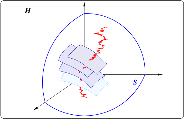
Figure 3: Interest rate dynamics. At each instant of time the interest rate term structure can be represented as a point on the positive orthant of the unit sphere ${\cal S}$ in the Hilbert space ${\cal H}=L^{2}({\bf R}_{+}^{1})$. The associated arbitrage-free interest rate dynamics gives rise to a stochastic trajectory on this space, which is foliated by hypersurfaces corresponding to level values of the short-term interest rate.

We would now like to interpret the Hilbert space dynamics in equation (7.80) more directly in a geometrical fashion. For this purpose we find it expedient to introduce an index notation, using Greek letters to signify Hilbert space operations (cf. Brody $\&$ Hughston 1998).

Thus if the function $\mathchar 28960\relax(x)$ is an element of ${\cal H}=L^{2}({\bf R}_{+}^{1})$, we denote it by $\mathchar 28960\relax^{\mathchar 28939\relax}$, and if $\mathchar 28967\relax(x)$ belongs to the dual Hilbert space ${\cal H}^{*}$ we denote this by $\mathchar 28967\relax_{\mathchar 28939\relax}$. Furthermore, their inner product is written

$$\mathchar 28960\relax^{\mathchar 28939\relax}\mathchar 28967\relax_{\mathchar 28939\relax}=\int_{0}^{\infty}\mathchar 28960\relax(x)\mathchar 28967\relax(x){\rm d}x.$$ (7.82)

There is a preferred symmetric quadratic form $g_{\mathchar 28939\relax\mathchar 28940\relax}$ on ${\cal H}$, given by $g_{\mathchar 28939\relax\mathchar 28940\relax}\mathchar 28960\relax^{\mathchar 28939\relax}\mathchar 28960\relax^{\mathchar 28940\relax}=\int_{0}^{\infty}(\mathchar 28960\relax(x))^{2}{\rm d}x$, which thus establishes an isomorphism between ${\cal H}$ and ${\cal H}^{*}$, given by $\mathchar 28960\relax^{\mathchar 28939\relax}\rightarrow\mathchar 28960\relax_{\mathchar 28939\relax}=g_{\mathchar 28939\relax\mathchar 28940\relax}\mathchar 28960\relax^{\mathchar 28940\relax}$. Intuitively, one can think of $g_{\mathchar 28939\relax\mathchar 28940\relax}$ as corresponding to the delta function $\mathchar 28942\relax(x,y)$, and then we have

$$g_{\mathchar 28939\relax\mathchar 28940\relax}\mathchar 28960\relax^{\mathchar 28939\relax}\mathchar 28967\relax^{\mathchar 28940\relax}=\int_{0}^{\infty}\mathchar 28960\relax(x)\mathchar 28942\relax(x,y)\mathchar 28967\relax(y){\rm d}x{\rm d}y.$$ (7.83)

There are a number of Hilbert space technicalities that have to be considered for a complete exposition of the matter, but that is not our immediate concern.

If $\mathchar 28952\relax(x)>0$ belongs to the positive orthant of $L^{2}({\bf R}^{1}_{+})$ then the corresponding indexed quantity $\mathchar 28952\relax^{\mathchar 28939\relax}$ has the interpretation of a ‘state vector’. In that case we can think of symmetric quadratic forms as representing certain classes of random variables. The expectation of the random variable $H_{\mathchar 28939\relax\mathchar 28940\relax}$ in the state $\mathchar 28952\relax^{\mathchar 28939\relax}$ is

$$E_{\mathchar 28952\relax}[H]=\frac{H_{\mathchar 28939\relax\mathchar 28940\relax}\mathchar 28952\relax^{\mathchar 28939\relax}\mathchar 28952\relax^{\mathchar 28940\relax}}{\mathchar 28952\relax_{\mathchar 28941\relax}\mathchar 28952\relax^{\mathchar 28941\relax}}.$$ (7.84)

Therefore, a state vector determines a mapping from random variables to real numbers, through (7.84). For a normalised state vector we have $\mathchar 28952\relax_{\mathchar 28939\relax}\mathchar 28952\relax^{\mathchar 28939\relax}=1$, although for some purposes it is convenient to relax the normalisation condition. In particular, we notice that the expectation (7.84) only depends on the direction of $\mathchar 28952\relax^{\mathchar 28939\relax}$.

Now suppose $\mathchar 28952\relax(x)$ is a positive function. In that case, the derivative $\partial_{x}$ can be thought of as a linear operator $D^{\mathchar 28939\relax}_{\ \mathchar 28940\relax}$ on ${\cal H}$, and we have an endomorphism given by $\mathchar 28952\relax^{\mathchar 28939\relax}\rightarrow D^{\mathchar 28939\relax}_{\ \mathchar 28940\relax}\mathchar 28952\relax^{\mathchar 28940\relax}$. By making use of this, we can now interpret, in the language of Hilbert space geometry, the first two terms appearing in the drift in the dynamical equation (7.80).

Let us begin by noting first that (5.48) can be rewritten in the form

$$\int_{0}^{\infty}\mathchar 28952\relax_{tx}\partial_{x}\mathchar 28952\relax_{tx}{\rm d}x=-\frac{1}{2}r_{t}.$$ (7.85)

This allows us to interpret the short term interest rate process $r_{t}$ in terms of the mean of the symmetric part of the operator $D^{\mathchar 28939\relax}_{\ \mathchar 28940\relax}$ in the state $\mathchar 28952\relax_{t}^{\mathchar 28939\relax}$, i.e.,

$$\frac{D_{\mathchar 28939\relax\mathchar 28940\relax}\mathchar 28952\relax^{\mathchar 28939\relax}_{t}\mathchar 28952\relax^{\mathchar 28940\relax}_{t}}{g_{\mathchar 28939\relax\mathchar 28940\relax}\mathchar 28952\relax^{\mathchar 28939\relax}_{t}\mathchar 28952\relax^{\mathchar 28940\relax}_{t}}=-\frac{1}{2}r_{t},$$ (7.86)

where $D_{\mathchar 28939\relax\mathchar 28940\relax}=g_{\mathchar 28939\relax\mathchar 28941\relax}D^{\mathchar 28941\relax}_{\ \mathchar 28940\relax}$. Therefore, if we let $D_{(\mathchar 28939\relax\mathchar 28940\relax)}$ denote the symmetric part of the operator $D^{\mathchar 28939\relax}_{\ \mathchar 28940\relax}$, then the abstract random variable in ${\cal H}$ corresponding to the short rate $r_{t}$ is given by $r_{\mathchar 28939\relax\mathchar 28940\relax}=-2D_{(\mathchar 28939\relax\mathchar 28940\relax)}$. Similarly we can represent the abstract random variable $x$ for the time left until maturity in ${\cal H}$ by a symmetric matrix $X_{\mathchar 28939\relax\mathchar 28940\relax}$. It is interesting to note that the random variables $X_{\mathchar 28939\relax\mathchar 28940\relax}$ for the maturity date and $r_{\mathchar 28939\relax\mathchar 28940\relax}$ for the short term interest rate are not ‘compatible’. Two random variables $A$ and $B$ are said to be compatible if the expression $\{\{A,C\},B\}-\{A,\{C,B\}\}$ vanishes for any random variable $C$, where $\{A,B\}=AB+BA$ denotes the anticommutator (Segal 1947). The lack of compatibility here indicates that the abstract probability system containing both $r_{\mathchar 28939\relax\mathchar 28940\relax}$ and $X_{\mathchar 28939\relax\mathchar 28940\relax}$ as random variables is not Kolmogorovian. However, the algebra of random variables generated by $X_{\mathchar 28939\relax\mathchar 28940\relax}$ is Kolmogorovian.

Now, let $\mathchar 28945\relax(x)$ be an arbitrary element of $L^{2}({\bf R}_{+}^{1})$, and let $\mathchar 28945\relax^{\mathchar 28939\relax}$ be the corresponding Hilbert space vector. Then clearly we have

$$\int_{0}^{\infty}\mathchar 28945\relax(x)\left[\partial_{x}\mathchar 28952\relax_{tx}+\mbox{$\textstyle\frac{1}{2}$}r_{t}\mathchar 28952\relax_{tx}\right]{\rm d}x=\mathchar 28945\relax_{\mathchar 28939\relax}\left[D^{\mathchar 28939\relax}_{\ \mathchar 28940\relax}\mathchar 28952\relax^{\mathchar 28940\relax}_{t}-\left(\frac{D_{\mathchar 28940\relax\mathchar 28941\relax}\mathchar 28952\relax^{\mathchar 28940\relax}_{t}\mathchar 28952\relax_{t}^{\mathchar 28941\relax}}{g_{\mathchar 28942\relax\mathchar 28943\relax}\mathchar 28952\relax_{t}^{\mathchar 28942\relax}\mathchar 28952\relax_{t}^{\mathchar 28943\relax}}\right)\mathchar 28952\relax^{\mathchar 28939\relax}_{t}\right].$$ (7.87)

In other words, the first two terms of the drift in (7.80) can be replaced by the expression ${\tilde{D}}^{\mathchar 28939\relax}_{\ \mathchar 28940\relax}\mathchar 28952\relax^{\mathchar 28940\relax}_{t}$, where

$${\tilde{D}}^{\mathchar 28939\relax}_{\ \mathchar 28940\relax}=D^{\mathchar 28939\relax}_{\ \mathchar 28940\relax}-\left(\frac{D_{\mathchar 28941\relax\mathchar 28942\relax}\mathchar 28952\relax^{\mathchar 28941\relax}_{t}\mathchar 28952\relax_{t}^{\mathchar 28942\relax}}{g_{\mathchar 28941\relax\mathchar 28942\relax}\mathchar 28952\relax_{t}^{\mathchar 28941\relax}\mathchar 28952\relax_{t}^{\mathchar 28942\relax}}\right)\mathchar 28942\relax^{\mathchar 28939\relax}_{\ \mathchar 28940\relax},$$ (7.88)

where $\mathchar 28942\relax^{\mathchar 28939\relax}_{\ \mathchar 28940\relax}$ is the Kronecker delta. Clearly, we have ${\tilde{D}}_{\mathchar 28939\relax\mathchar 28940\relax}\mathchar 28952\relax^{\mathchar 28939\relax}\mathchar 28952\relax^{\mathchar 28940\relax}=0$.

With this in mind, let us now proceed to the interpretation of the volatility process $\mathchar 28955\relax_{tx}$. Again, $\mathchar 28955\relax_{tx}$ has the character of a linear operator acting on $\mathchar 28952\relax_{tx}$, subject to the constraint $E_{\mathchar 28954\relax}[\mathchar 28955\relax_{tx}]=0$. This can be consistently enforced if there exists a symmetric process $\mathchar 28951\relax_{t\mathchar 28939\relax\mathchar 28940\relax}$ such that

$$\int_{0}^{\infty}\mathchar 28945\relax(x)\mathchar 28952\relax_{tx}\mathchar 28955\relax_{tx}{\rm d}x=\mathchar 28945\relax^{\mathchar 28939\relax}\left(\mathchar 28951\relax_{t\mathchar 28939\relax\mathchar 28940\relax}\mathchar 28952\relax^{\mathchar 28940\relax}_{t}-E_{\mathchar 28952\relax}[\mathchar 28951\relax_{t}]\mathchar 28952\relax_{t\mathchar 28939\relax}\right).$$ (7.89)

The symmetric operator-valued random process $\mathchar 28951\relax_{t\mathchar 28939\relax\mathchar 28940\relax}$, whose existence is thus implied, is ‘primitive’ in the sense that it is unconstrained and can be specified exogenously. If we write

$$\mathchar 28955\relax_{t\mathchar 28939\relax\mathchar 28940\relax}=\mathchar 28951\relax_{t\mathchar 28939\relax\mathchar 28940\relax}-E_{\mathchar 28952\relax}[\mathchar 28951\relax_{t}]g_{\mathchar 28939\relax\mathchar 28940\relax},$$ (7.90)

we obtain

$$\int_{0}^{\infty}\mathchar 28945\relax(x)\mathchar 28952\relax_{tx}\mathchar 28955\relax_{tx}{\rm d}x=\mathchar 28945\relax_{\mathchar 28939\relax}\mathchar 28955\relax_{t\mathchar 28940\relax}^{\mathchar 28939\relax}\mathchar 28952\relax^{\mathchar 28940\relax}_{t},$$ (7.91)

and also

$$\int_{0}^{\infty}\mathchar 28945\relax(x)\mathchar 28952\relax_{tx}\mathchar 28955\relax_{tx}^{2}{\rm d}x=\mathchar 28945\relax_{\mathchar 28939\relax}\mathchar 28955\relax_{t\mathchar 28940\relax}^{\mathchar 28939\relax}\mathchar 28955\relax_{t\mathchar 28941\relax}^{\mathchar 28940\relax}\mathchar 28952\relax^{\mathchar 28941\relax}_{t}.$$ (7.92)

Therefore, putting the various ingredients together, we obtain:

Proposition 5

The dynamics of the Hilbert space vector $\mathchar 28952\relax^{\mathchar 28939\relax}_{t}$ that characterises the term structure in an admissible, arbitrage-free interest rate framework is governed by the stochastic differential equation

$${\rm d}\mathchar 28952\relax^{\mathchar 28939\relax}_{t}=\left({\tilde{D}}^{\mathchar 28939\relax}_{\ \mathchar 28940\relax}-\mbox{$\textstyle\frac{1}{8}$}\mathchar 28955\relax^{\mathchar 28939\relax}_{t\mathchar 28941\relax}\cdot\mathchar 28955\relax^{\mathchar 28941\relax}_{t\mathchar 28940\relax}\right)\mathchar 28952\relax^{\mathchar 28940\relax}_{t}{\rm d}t+\mbox{$\textstyle\frac{1}{2}$}\mathchar 28955\relax^{\mathchar 28939\relax}_{t\mathchar 28940\relax}\mathchar 28952\relax^{\mathchar 28940\relax}_{t}\cdot\left({\rm d}W_{t}+\mathchar 28949\relax_{t}{\rm d}t\right),$$ (7.93)

where ${\tilde{D}}^{\mathchar 28939\relax}_{\ \mathchar 28940\relax}$ is given as in (7.88), and the adapted operator-valued process $\mathchar 28955\relax_{t\mathchar 28939\relax\mathchar 28940\relax}$ is expressible in the form

$$\mathchar 28955\relax_{t\mathchar 28939\relax\mathchar 28940\relax}=\mathchar 28951\relax_{t\mathchar 28939\relax\mathchar 28940\relax}-\left(\frac{\mathchar 28951\relax_{\mathchar 28941\relax\mathchar 28942\relax}\mathchar 28952\relax^{\mathchar 28941\relax}_{t}\mathchar 28952\relax_{t}^{\mathchar 28942\relax}}{g_{\mathchar 28941\relax\mathchar 28942\relax}\mathchar 28952\relax_{t}^{\mathchar 28941\relax}\mathchar 28952\relax_{t}^{\mathchar 28942\relax}}\right)g_{\mathchar 28939\relax\mathchar 28940\relax},$$ (7.94)

where $\mathchar 28951\relax_{t\mathchar 28939\relax\mathchar 28940\relax}$ is an arbitrary adapted operator-valued process.

This result shows that the evolution of the yield curve can be viewed consistently as a process on the positive orthant of the unit sphere in Hilbert space, and thus gives rise to an entirely new way of understanding the dynamics of the term structure. The purpose of the quadratic term in the drift of (7.93) is to keep the process on the sphere, and in the absence of the term involving the operator $D^{\mathchar 28939\relax}_{\ \mathchar 28940\relax}$ we would have a general local martingale on the sphere ${\cal S}$ with respect to the risk-neutral measure, where the martingale property on ${\cal S}$ is characterised in a standard way by use of the techniques of stochastic differential geometry (see, e.g., Emery 1989, Ikeda $\&$ Watanabe 1989, Hughston 1996). The term involving the operator $D^{\mathchar 28939\relax}_{\ \mathchar 28940\relax}$ splits into a symmetric and an antisymmetric part. The drift generated by the antisymmetric part of $D^{\mathchar 28939\relax}_{\ \mathchar 28940\relax}$ is generated by a symmetry of the sphere ${\cal S}$. The drift generated by the symmetric part of $D^{\mathchar 28939\relax}_{\ \mathchar 28940\relax}$, on the other hand, is a negative gradient vector field orthogonal to surfaces in ${\cal S}$ generated by level values of the short rate $r_{t}$. This term therefore creates a tendency for the vector $\mathchar 28952\relax^{\mathchar 28939\relax}$ to drift towards a lower interest rate, a property of the negative gradient field which is then counterbalanced by the effects of the diffusive term.

Acknowledgements

LPH acknowledges the hospitality of the Finance Department of the Graduate School of Business of the University of Texas at Austin, where part of this work was carried out. DCB gratefully acknowledges financial support from The Royal Society.

References

1
2Amari, S. (1985) Differential-Geometric
Methods in Statistics (Springer-Verlag, Berlin).
3
4Bhattacharyya, A. (1943) Proc. 29th Indian Sci.
Cong. 3, 13.
5
6Baxter, M. (1997) General Interest Rate Models, in
Mathematics of Derivative Securities, eds.
Dempster, M. A. H. Pliska, S. R. (Cambridge University
Press, Cambridge).
7
8Björk, T. Svensson, L. (1999) On the existence
of finite dimensional realisations for nonlinear forward rate
models (Preprint, Stockholm School of Economics).
9
10Björk, T. Christensen, B. J. (1999)
Mathematical Finance, 9, 323.
11
12Björk, T. Gombani, A. (1999)
Finance and Stochastics, 3, 413.
13
14Björk, T. (2000)
A Geometric View of Interest Rate Theory.
To appear in Handbook of Mathematical Finance
(Cambridge University Press, Cambridge).
15
16Brace, A., Gatarek, D. Musiela, M. (1996)
The Market Model of Interest Rate Dynamics, in Vasicek
and Beyond: Approach to Building and Applying Interest Rate
Models, ed. Hughston, L. P. (Risk Publications, London).
17
18Brace, A., Gatarek, D. Musiela, M. (1997)
Math. Finance 7, 125.
19
20Brody, D. C. (2000) Mathematical Theory of Finance
(Nihon-Hyoronsya, Tokyo).
21
22Brody, D. C. Hughston, L. P. (1998) Proc.
Roy. Soc. London 454, 2445.
23
24Burbea, J. (1986) Expo. Math. 4, 347.
25
26Carverhill, A. (1994) Stochast. Rep. 53, 227.
27
28Cox, J. C., Ingersoll, J. Ross, S. (1985)
Econometrica 53, 385.
29
30Dawid, A. P. (1977) Ann. Statist. 5, 1249.
31
32Emery, M. (1989) Stochastic Calculus on
Manifolds (Springer-Verlag, Berlin).
33
34Fisher, R. A. (1921) Phil. Trans. Roy. Soc. A
222, 309.
35
36Flesaker, B. Hughston, L. P. (1996) Risk
Magazine 9, 46.
37
38Flesaker, B. Hughston, L. P. (1997a)
Exotic Interest Rate Options, in Exotic Options:
the State of the Art, eds. Clewlow, L. Strickland, C.
(International Thompson Press, London).
39
40Flesaker, B. Hughston, L. P. (1997b)
Dynamic Models of Yield Curve Evolution, in Mathematics of Derivative Securities, eds. Dempster, M. A. H.
Pliska, S. R. (Cambridge University Press, Cambridge).
41
42Flesaker, B. Hughston, L. P. (1997c) Net
Exposure 3, 55.
43
44Harrison, J. M. Kreps, D. M. (1979) J. Econom.
Theory 20, 381.
45
46Harrison, J. M. Pliska, S. R. (1981) Stochast.
Proc. Appl. 11, 215.
47
48Heath, D., Jarrow, R. Morton, A. (1992)
Econometrica 60, 77.
49
50Ho, T. S. Y. Lee, S.B. (1986) J. Finance 41,
1011.
51
52Hughston, L. P. (1996a) Proc. Roy. Soc. London
452, 953.
53
54Hughston, L. P. (1996) Introduction, in
Vasicek and Beyond: Approaches to Building and Applying
Interest Rate Models, ed. Hughston, L. P. (Risk Publications,
London).
55
56Hunt, P. J. Kennedy, J. E. (2000) Financial
Derivatives in Theory and Practice (Wiley, Chichester)
57
58Ikeda, N. Watanabe, S. (1989) Stochastic
Differential Equations and Diffusion Process (North-Holland,
Amsterdam).
59
60Jamshidian, F. (1997) Finance and Stochastics 1,
293.
61
62Kass, R. E. (1989) Statist. Sci. 4, 188.
63
64Kennedy, D. (1994) Math. Finance 4, 247.
65
66Mahalanobis, P. C. (1936) Proc. Nat. Inst. Sci. India
A 2, 49.
67
68Merton, R. C. (1973) Bell. J. Econ. Manag. Sci. 4,
141.
69
70Murray, M. K. Rice, J. W. (1993) Differential
Geometry and Statistics (Chapman Hall, London).
71
72Musiela, M. Rutkowski, M. (1997) Martingale
Methods in Financial Modelling (Springer-Verlag, Berlin).
73
74Nielsen, L. T. (1999) Pricing and Hedging of
Derivative Securities (Oxford University Press, Oxford).
75
76Rao, C. R. (1945) Bull. Calcutta Math. Soc.
37, 81.
77
78Rogers, L. C. G. (1994) Which model of the term
structure of interest rate should one use?, in Mathematical Finance, IMA 65, 63. (Springer-Verlag,
Berlin).
79
80Rogers, L. C. G. (1997) Math. Finance 7, 157.
81
82Santa-Clara, P. Sornette, D. (1997) The dynamics
of the forward interest rate curve with stochastic string
shocks (Preprint, University of California at Los Angeles).