Oceanic three-dimensional Lagrangian Coherent Structures:
A study of a mesoscale eddy in the Benguela ocean region.

Abstract

We study three dimensional oceanic Lagrangian Coherent Structures (LCSs) in the Benguela region, as obtained from an output of the ROMS model. To do that we first compute Finite-Size Lyapunov exponent (FSLE) fields in the region volume, characterizing mesoscale stirring and mixing. Average FSLE values show a general decreasing trend with depth, but there is a local maximum at about 100 m depth. LCSs are extracted as ridges of the calculated FSLE fields. They present a “curtain-like” geometry in which the strongest attracting and repelling structures appear as quasivertical surfaces. LCSs around a particular cyclonic eddy, pinched off from the upwelling front are also calculated. The LCSs are confirmed to provide pathways and barriers to transport in and out of the eddy.

1 Introduction.

Mixing and transport processes are fundamental to determine the physical, chemical and biological properties of the oceans. From plankton dynamics to the evolution of pollutant spills, there is a wide range of practical issues that benefit from a correct understanding and modeling of these processes. Although mixing and transport in the oceans occur in a wide range of scales, mesoscale and sub-mesoscale variability are known to play a very important role (Thomas et al., 2008; Klein and Lapeyre, 2009).

Mesoscale eddies are especially important in this aspect because of their long life in oceanic flows, and their stirring and mixing properties. In the southern Benguela, for instance, cyclonic eddies shed from the Agulhas current can transport and exchange warm waters from the Indian Ocean to the South Atlantic (Byrne et al., 1995; Lehahn et al., 2011). Moreover, mesoscale eddies have been shown to drive important biogeochemical processes in the ocean such as the vertical flux of nutrients into the euphotic zone (McGillicuddy et al., 1998; Oschlies and Garçon, 1998). Another effect of eddy activity seems to be the intensification of mesoscale and sub-mesoscale variability due to the filamentation process where strong tracer gradients are created by the stretching of tracers in the shear- and strain-dominated regions in between eddy cores (Elhmaïdi et al., 1993). Studies of the vertical structure of such eddies in the Benguela region (e. g. Doglioli et al. (2007) and Rubio et al. (2009)) have shown that they can extended to one thousand meters deep waters.

In the last decades new developments in the description and modelling of oceanic mixing and transport from a Lagrangian viewpoint have emerged (Mariano et al., 2002; Lacasce, 2008). These Lagrangian approaches have become more and more frequent due to the increased availability of detailed knowledge of the velocity field from Lagrangian drifters, satellite measurements and computer models. In particular, the very relevant concept of Lagrangian Coherent Structure (LCS) (Haller, 2000; Haller and Yuan, 2000) is becoming crucial for the analysis of transport in flows. LCSs are structures that separate regions of the flow with different dynamical behavior. They give a general geometric view of the dynamics, acting as a (time-dependent) roadmap for the flow. They are templates serving as proxies to, for instance, barriers and avenues to transport or eddy boundaries (Boffetta et al., 2001; Haller and Yuan, 2000; Haller, 2002; d’Ovidio et al., 2004, 2009; Mancho et al., 2006).

The relevance of the three-dimensional structure of LCSs begins to be unveiled in atmospheric contexts (du Toit and Marsden, 2010; Tang et al., 2011; Tallapragada et al., 2011). In the case of oceanic flows, however, the identification of the LCSs and the study of their role on biogeochemical tracers transport has been mostly restricted to the marine surface (d’Ovidio et al., 2004; Waugh et al., 2006; d’Ovidio et al., 2009; Beron-Vera et al., 2008). This is mainly due to two reasons: a) tracer vertical displacement is usually very small with respect to the horizontal one; and b) satellite data of any quantity (temperature, chlorophyll, altimetry for velocity, etc..) are only available from the observation of the ocean surface.

Oceanic flows can be considered mainly two-dimensional, because there is a great disparity between the horizontal and vertical length scales, and they are strongly stratified due to the Earth’s rotation. There are, however, areas in the ocean where vertical motions are fundamental. Firstly there are the so-called upwelling regions, which are the most biologically active marine zones in the world (Rossi et al., 2008; Pauly and Christensen, 1995). The reason is that due to an Ekmann pumping mechanism close to the coast, there is a surface uprising of deep cold waters rich in nutrients, inducing a high proliferation of plankton concentration. Typically, vertical velocities in upwelling regions are much larger than in open ocean, but still one order of magnitude smaller than horizontal velocities. Another example where there are significant vertical processes are mesoscale eddies producing submesoscale structures (frontogenesis), which are responsible for strong ageostrophic vertical process, in addition to the vertical exchange thought to occur at the eddy interior (Klein and Lapeyre, 2009). Thus, the identification of the three-dimensional (3d) LCSs in these areas is crucial, as well as understanding their correlations with biological activity. Another reason to include the third dimension in LCS studies is to investigate the vertical variation in their properties.

The main objective of this paper is the characterization of 3d LCSs, extracted in an upwelling region, the Benguela area in the Southern Atlantic Ocean. For this goal we use Finite-Size Lyapunov Exponents (FSLEs). FSLEs (Aurell et al., 1997; Artale et al., 1997) measure the separation rate of fluid particles between two given distance thresholds. LCSs are computed as the ridges of the FSLE field (d’Ovidio et al., 2004; Molcard et al., 2006; Haza et al., 2008; d’Ovidio et al., 2009; Poje et al., 2010; Haza et al., 2010). The rigorous definition of LCS as ridges of a Lagrangian stretching measure was given for the Finite-Time Lyapunov Exponents (FTLE) in Shadden et al. (2005) and Lekien et al. (2007), which are closely related to FSLEs. More recently, hyperbolic LCS have been defined independently of such stretching measures by Haller (2011). Following many previous studies (d’Ovidio et al., 2004; Molcard et al., 2006; d’Ovidio et al., 2009; Branicki and Wiggins, 2009) we adopt the mathematical results for Finite-Time Lyapunov Exponents (FTLE) to FSLE, assuming them to be valid. In particular, we assume that LCS are identified with ridges (Haller, 2001), i.e., the local extrema of the FTLE field, and also we expect, in accordance to the results in Shadden et al. (2005) and Lekien et al. (2007) for FTLEs, that the material flux through these LCS is small and that they are transported by the flow as quasi-material surfaces.

To confirm that our identification of LCSs with ridges of the FSLE field, we perform (in Sect. III) direct particle trajectory integrations that show that the computed LCS really organize the tracer flow. In our work, we will emphasize the numerical methodology since up to now FSLEs have only been computed for the marine surface (an exception is Özgökmen et al. (2011)). We then focus on a particular eddy very prominent in the area at the chosen temporal window and study the stirring and mixing on it’s vicinity. Some previous results for Lagrangian eddies were obtained by Branicki and Kirwan (2010) and Branicki et al. (2011), applying the methodology of lobe dynamics and the turnstile mechanism to eddies pinched off from the Loop Current. In this paper we focus on FSLE fields and the associated particle trajectories to study transport in and out of the chosen mesoscale eddy. Since this is a first attempt to study 3d oceanic LCS, more general results (on Benguela and other upwelling regions) are left for future work.

To circumvent the lack of appropriate observational data in the vertical direction, we use velocity fields from a numerical simulation. They are high resolution simulations from the ROMS model (see section 2 below) thus appropriate to study regional-medium scale basins.

The paper is organized as follows: In section II we describe the data and methods. In section III we present our results. Section IV contains a discussion of the results and Section V summarizes our conclusions.

2 Data and Methods.

2.1 Velocity data set.

The Benguela ocean region is situated off the west coast of southern Africa. It is characterized by a vigorous coastal upwelling regime forced by equatorward winds, a substantial mesoscale activity of the upwelling front in the form of eddies and filaments, and also by the northward drift of Agulhas eddies.

The velocity data set comes from a regional ocean model simulation of the Benguela Region (Le Vu et al., 2011). ROMS (Shchepetkin and McWilliams, 2003, 2005) is a split-explicit free-surface, topography following model. It solves the incompressible primitive equations using the Boussinesq and hydrostatic approximations. Potential temperature and salinity transport are included by coupling advection/diffusion schemes for these variables. The model was forced with climatological data. The data set area extends from 12°S to 35°S and from 4°E to 19°E (see Fig. 1). The velocity field $\mathbf{u}=(u,v,w)$ consists of two years of daily averaged zonal ($u$), meridional ($v$), and vertical velocity ($w$) components, stored in a three-dimensional grid with an horizontal resolution of $1/12$ degrees $\sim 8$ km, and $32$ vertical terrain-following levels using a stretched vertical coordinate where the layer thickness varies, increasing from the surface to the ocean interior. Since the ROMS model considers the hydrostatic approximation it is important to note that Mahadevan (2006), when comparing results from non-hydrostatic and hydrostatic versions of the same model of vertical motions at submesoscale fronts, found that while instantaneous vertical velocities structures differ, the averaged vertical flux is similar in both hydrostatic and non-hydrostatic simulations.

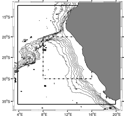
Figure 1: Benguela ocean region. The velocity field domain is limited by the continuous black line. The FSLE calculation area is limited by the dash-dot black line. Bathymetric contour lines are from ETOPO1 global relief model (Amante and Eakins, 2009) starting a 0 m depth up to 4000 m at 500 m interval.

2.2 Finite-Size Lyapunov Exponents.

In order to study non-asymptotic dispersion processes such as stretching at finite scales and time intervals, the Finite Size Lyapunov Exponent (Aurell et al., 1997; Artale et al., 1997) is particularly well suited. It is defined as:

$$\lambda=\frac{1}{\tau}\log\frac{\delta_{f}}{\delta_{0}},$$ (1)

where $\tau$ is the time it takes for the separation between two particles, initially $\delta_{0}$, to reach $\delta_{f}$. In addition to the dependence on the values of $\delta_{0}$ and $\delta_{f}$, the FSLE depends also on the initial position of the particles and on the time of deployment. Locations (i.e. initial positions) leading to high values of this Lyapunov field identify regions of strong separation between particles, i.e., regions that will exhibit strong stretching during evolution, that can be identified with the LCS (Boffetta et al., 2001; d’Ovidio et al., 2004; Joseph and Legras, 2002).

In principle, for computing FSLEs in three dimensions one just needs to extend the method of d’Ovidio et al. (2004), that is, one needs to compute the time that fluid particles initially separated by $\delta_{0}=[(\delta x_{0})^{2}+(\delta y_{0})^{2}+(\delta z_{0})^{2}]^{1/2}$ need to reach a final distance of $\delta_{f}=[(\delta x_{f})^{2}+(\delta y_{f})^{2}+(\delta z_{f})^{2}]^{1/2}$. The main difficulty in doing this is that in the ocean vertical displacements (even in upwelling regions) are much smaller than the horizontal ones, and so do not contribute significantly to total particle dispersion (Özgökmen et al., 2011). By the time the horizontal particle dispersion has scales of tenths or hundreds of kilometers (typical mesoscale structures are studied using $\delta_{f}\approx 100km$ (d’Ovidio et al., 2004)), particle dispersion in the vertical can have at most scales of hundreds of meters and usually less. This means that the vertical separation will not contribute significantly to the accumulated distance between particles. In addition, since length scales in the horizontal and vertical differ by several orders of magnitude, one faces the impossibility of assigning equal $\delta_{0}$ to the horizontal and vertical particle pairs. It should be noted however that these shortcomings arise from the different scales of length and time that characterize horizontal and vertical dispersion processes in the ocean, and so should not be seem as intrinsic limitations of the method. For non-oceanic flows a direct generalization of FSLEs is straightforward.

Thus, in this paper we implemented a quasi three-dimensional computation of FSLEs. That is, we make the computation for every (2d) ocean layer, but where the particle trajectories calculation use the full 3d velocity field. I.e., at each level (depth) we set $\delta z_{O}=0$, and the final distance is computed without taking the vertical distance between particles. It is important to note that, since we allow the particles to evolve in the full 3d velocity field, we take into account vertical quantities such as vertical velocity shear that may influence the horizontal separation between particle pairs.

There are other possible approaches to the issue of different scales in the vertical and horizontal. One way is to assign anisotropic initial and final displacements in the FSLE calculation (i. e., including a $\delta z_{0}$ and $\delta z_{f}$ much smaller than the horizontal initial and final separations). A second approach is to use different weights for the horizontal and vertical separations in the calculations of the distance, perhaps in combination with the first. We have cheked both alternatives and found that, with reasonable choices of initial and final distances and distance metrics, the results were equivalent to the quasi-3d computation. The reason is that actual dispersion is primarily horizontal as commented above.

More in detail, a grid of initial locations $\textbf{x}_{0}$ in the longitude/latitude/depth geographical space $(\phi,\theta,z)$, fixing the spatial resolution of the FSLE field, is set up at time $t$. The horizontal distance among the grid points, $\delta_{0}$, was set to $1/36$ degrees ($\approx 3$ km), i.e. three times finer resolution than the velocity field (Hernandez-Carrasco et al., 2011), and the vertical resolution (distance between layers) was set to $20$ m in order to have a good representation of the vertical variations in the FSLE field. Particles are released from each grid point and their three dimensional trajectories calculated. The distances of each particle with respect to the ones that were initially neighbors at an horizontal distance $\delta_{0}$ are monitored until one of the horizontal separations reaches a value $\delta_{f}$. By integrating the three dimensional particle trajectories backward and forward in time, we obtain the two different types of FSLE maps: the attracting LCS (for the backward), and the repelling LCS (forward) (d’Ovidio et al., 2004; Joseph and Legras, 2002). We obtain in this way FSLE fields with a horizontal spatial resolution given by $\delta_{0}$. The final distance $\delta_{f}$ was set to $100$ km, which is, as already mentioned, a typical length scale for mesoscale studies. The trajectories were integrated for a maximum of $T=178$ days (approximately six months) using an integration time step of $6$ hours. When a particle reached the coast or left the velocity field domain, the FSLE value at its initial position and initial time was set to zero. If the interparticle horizontal separation remains smaller than $\delta_{f}$ during all the integration time, then the FSLE for that location is also set to zero.

The equations of motion that describe the evolution of particle trajectories are

$$\frac{d\phi}{dt} = \frac{1}{R_{z}}\frac{u(\phi,\theta,z,t)}{cos(\theta)},$$ (2)

$$\frac{d\theta}{dt} = \frac{1}{R_{z}}v(\phi,\theta,z,t),$$ (3)

$$\frac{dz}{dt} = w(\phi,\theta,z,t),$$ (4)

where $\phi$ is longitude, $\theta$ is latitude and $z$ is the depth. $R_{z}$ is the radial coordinate of the moving particle $R_{z}=R-z$, with $R=6371$ km the mean Earth radius. For all practical purposes, $R_{z}\approx R$. Particle trajectories are integrated using a $4^{th}$ order Runge-Kutta method. For the calculations, one needs the (3d) velocity values at the current location of the particle. Since the six grid nodes surrounding the particle do not form a regular cube, direct trilinear interpolation can not be used. Thus, an isoparametric element formulation is used to map the nodes of the velocity grid surrounding the particles position to a regular cube, and an inverse isoparametric mapping scheme (Yuan et al., 1994) is used to find the coordinates of the interpolation point in the regular cube coordinate system.

2.3 Lagrangian Coherent Structures.

In 2d, LCS practically coincide with (finite-time) stable and unstable manifolds of relevant hyperbolic structures in the flow (Haller, 2000; Haller and Yuan, 2000; Joseph and Legras, 2002). The structure of these last objects in 3d is generally much more complex than in 2d (Haller, 2001; Pouransari et al., 2010), and they can be locally either lines or surfaces. As commented before, however, vertical motions in the ocean are slow. Thus, at each fluid parcel the strongest attracting and repelling directions should be nearly horizontal. This, combined with the incompressibility property, implies that the most attracting and repelling regions (i.e. the LCSs) should appear as almost vertical surfaces, since the attraction or repulsion should occur normally to the LCS. As a consequence, the LCSs will have a “curtain-like” geometry, with deviations from the vertical due to either the orientation of the most attracting or repelling direction deviating from the horizontal, or when strong vertical shear produces variations along the vertical in the most repelling or attracting regions in the flow. We expect the LCS sheet-like objects to coincide with the strongest hyperbolic manifolds when these are two dimensional, and to contain the strongest hyperbolic lines.

The curtain-like geometry of the LCS was already commented in Branicki and Malek-Madani (2010), Branicki and Kirwan (2010), or Branicki et al. (2011). In the latter paper it was shown that, in a 3d flow, these structures would appear mostly vertical when the ratio of vertical shear of the horizontal velocity components to the average horizontal velocities is small. This ratio also determines the vertical extension of the structures. In Branicki and Kirwan (2010), the argument was used to construct a 3d picture of hyperbolic structures from the computation in a 2d slice. In the present paper we confirm the curtain-like geometry of the LCSs, and show that they are relevant to organize the fluid flow in this realistic 3d oceanic setting. This is done in the next section by comparing actual particle trajectories with the computed LCSs.

Differently than 2d, where LCS can be visually identified as the maxima of the FSLE field, in 3d the ridges are hidden within the volume data. Thus, one needs to explicitly compute and extract them, using the definition of LCSs as the ridges of the FSLEs. A ridge $L$ is a co-dimension 1 orientable, differentiable manifold (which means that for a three-dimensional domain $D$, ridges are surfaces) satisfying the following conditions (Lekien et al., 2007):

1. The field $\lambda$ attains a local extremum at $L$.

2. The direction perpendicular to the ridge is the direction of fastest descent of $\lambda$ at $L$.

Mathematically, the two previous requirements can be expressed as

$$\mathbf{n}^{\mathrm{T}}\nabla\lambda = 0,$$ (5)

$$\mathbf{n}^{\mathrm{T}}\mathbf{H}\mathbf{n}=\min_{\lVert\mathbf{u}\rVert=1}\mathbf{u}^{\mathrm{T}}\mathbf{H}\mathbf{u} < 0,$$ (6)

where $\nabla\lambda$ is the gradient of the FSLE field $\lambda$, $\mathbf{n}$ is the unit normal vector to $L$ and $\mathbf{H}$ is the Hessian matrix of $\lambda$.

The method used to extract the ridges from the scalar field $\lambda(\mathbf{x}_{0},t)$ is from Schultz et al. (2010). It uses an earlier (Eberly et al., 1994) definition of ridge in the context of image analysis, as a generalized local maxima of scalar fields. For a scalar field $f:\mathbb{R}^{n}\rightarrow\mathbb{R}$ with gradient $\mathbf{g}=\nabla f$ and Hessian $\mathbf{H}$, a d-dimensional height ridge is given by the conditions

$$\forall_{d<i\leq n}\quad\mathbf{g}^{\mathrm{T}}\mathbf{e}_{i}=0\ \textrm{and}\ \alpha_{i}<0,$$ (7)

where $\alpha_{i},i\in\{1,2,\dotsc,n\}$, are the eigenvalues of $\mathbf{H}$, ordered such that $\alpha_{1}\geq\dotsc\geq\alpha_{n}$, and $\mathbf{e}_{i}$ is the eigenvector of $\mathbf{H}$ associated with $\alpha_{i}$. For $n=3$, (7) becomes

$$\mathbf{g}^{\mathrm{T}}\mathbf{e}_{3}=0\ \textrm{and}\ \alpha_{3}<0.$$ (8)

This ridge definition is equivalent to the one given by (5) since the unit normal $\mathbf{n}$ is the eigenvector (when normalized) associated with the minimum eigenvalue of $\mathbf{H}$. In other words, in $\mathbb{R}^{3}$ the $\mathbf{e}_{1},\mathbf{e}_{2}$ eigenvectors point locally along the ridge and the $\mathbf{e}_{3}$ eigenvector is orthogonal to it.

The ridges extracted from the backward FSLE map approximate the attracting LCS, and the ridges extracted from the forward FSLE map approximate the repelling LCS. The attracting ones are the more interesting from a physical point of view (d’Ovidio et al., 2004, 2009), since particles (or any passive scalar driven by the flow) typically approach them and spread along them, giving rise to filament formation. In the extraction process it is necessary to specify a threshold $s$ for the ridge strength $|\alpha_{3}|$, so that ridge points whose value of $\alpha_{3}$ is lower (in absolute value) than $s$ are discarded from the extraction process. Since the ridges are constructed by triangulations of the set of extracted ridge points, the $s$ threshold greatly determines the size and shape of the extracted ridge, by filtering out regions of the ridge that have low strength. The reader is referred to Schultz et al. (2010) for details about the ridge extraction method. The height ridge definition has been used to extract LCS from FTLE fields in several works (see, among others, Sadlo and Peikert (2007)).

3 Results

3.1 Three dimensional FSLE field

The three dimensional FSLE field was calculated for a $30$ day period starting September 17, with snapshots taken every $2$ days. The fields were calculated for an area of the Benguela ocean region between latitudes 20°S and 30°S and longitudes 8°E to 16°E (see figure 1). The area is bounded at NW by the Walvis Ridge and the continental slope approximately bisects the region from NW to SE. The western half of the domain has abyssal depths of about 4000 m. The calculation domain extended vertically from $20$ up to $580$ m of depth. Both backward and forward calculations were made in order to extract the attracting and repelling LCS.

Figure 2: Vertical profile of 30 day average backward and forward FSLE. The 30 day average field was spatially averaged at each layer over the FSLE calculation area to produce the vertical profiles. The backward FSLE average is shown in continuous and the forward FSLE is shown in dashed.

Figure 2 displays the vertical profile of the average FSLE for the 30 day period. There are small differences between the backward and the forward values due to the different intervals of time involved in their calculation. But both profiles have a similar shape and show a general decrease with depth. There is a notable peak in the profiles at about 100 m depth that indicates increased mesoscale variability (and transport, as shown in Sect. 3.2 at that depth).

A snapshot of the attracting LCSs for day 1 of the calculation period is shown in figure 3. As expected, the structures appear as thin vertical curtains, most of them extending throughout the depth of the calculation domain. The area is populated with LCS, denoting the intense mesoscale activity in the Benguela region. As already mentioned, in three dimensions the ridges are not easily seen, since they are hidden in the volume data. However the horizontal slices of the field in figure 3 show that the attracting LCS fall on the maximum backward FSLE field lines of the 2d slices. The repelling LCS (not shown) also fall on the maximum forward FSLE field lines of the 2d slices.

Figure 3: Attracting LCS (blue) for day 1 of the calculation period, together with horizontal slices of the backward FSLE field at 120 m and 300 m depth. Colorbar refers to colormap of horizontal slices. The units of the colorbar are $day^{-1}$.

Since the $\lambda$ value of a point on the ridge and the ridges strength $\alpha_{3}$ are only related through the expressions (7) and (8), the relationship between the two quantities is not direct. This creates a difficulty in choosing the appropriate strength threshold for the extraction process. A too small value of $s$ will result in very small LCS that appear to have little influence on the dynamics, while a greater value will result in only a partial rendering of the LCS, limiting the possibility of observing their real impact on the flow. Computations with several values of $s$ lead us to the optimum choice $s=20\>day^{-1}m^{-2}$, meaning that grid nodes with $\alpha_{3}<-20\>day^{-1}m^{-2}$ were filtered out from the LCS triangulation.

We have seen in this section an example of how the ridges of the $3d$ FSLE field, the LCS, distribute in the Benguela ocean region. Their ubiquity shows their impact on the transport and mixing properties. In the next section we concentrate on the properties of a single 3d mesoscale eddy.

3.2 Study of the dynamics of a relevant mesoscale eddy

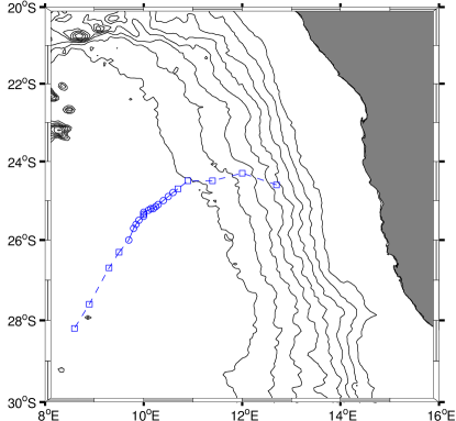
Figure 4: Trajectory (advancing from NE to SW) of the eddy center inside the calculation domain. Circles indicate the center location during the 30 day FSLE calculation period, and squares previous and posterior positions. Bathymetric lines same as in figure 1.

Let us study a prominent cyclonic eddy observed in the data set. The trajectory of the center of the eddy was tracked and it is shown in figure 4. The eddy was apparently pinched off at the upwelling front. At day $1$ of the FSLE calculation period its center was located at latitude 24.8°S and longitude 10.6°E, leaving the continental slope, and having a diameter of approximately $100$ km. One may ask: what is its vertical size? is it really a barrier, at any depth, for particle transport?

To properly answer these questions the eddy, in particular its frontiers, should be located. From the Eulerian point of view it is commonly accepted that eddies are delimited by closed contours of vorticity and that the existence of strong vorticity gradients prevent the transport in and out of the eddy. Such transport may occur when the eddy is destroyed or undergoes strong interactions with other eddies (Provenzale, 1999). In a Lagrangian view point, however, an eddy can be defined as a region delimited by intersections and tangencies of LCS, whether in 2d or 3d space. The eddy itself is an elliptic structure (Haller and Yuan, 2000; Branicki and Kirwan, 2010; Branicki et al., 2011). In this Lagrangian view of an eddy, the transport inhibition to and from the eddy is now related to the existence of these transport barriers delimiting the eddy region, which are known to be quasi impermeable.

Using the first approach, i.e., the Eulerian view, the vertical distribution of the $Q$-criteria (Hunt et al., 1988; Jeong and Hussain, 1995) was used to determine the vertical extension of the mesoscale eddy. The $Q$ criterium is a 3d version of the Okubo-Weiss criterium (Okubo, 1970; Weiss, 1991) and measures the relative strength of vorticity and straining. In this context, eddies are defined as regions with positive $Q$, with $Q$ the second invariant of the velocity gradient tensor

$$Q=\frac{1}{2}(\|\mathbf{\Omega}\|^{2}-\|\mathbf{S}\|^{2}),$$ (9)

where $\|\mathbf{\Omega}\|^{2}=tr(\mathbf{\Omega}\mathbf{\Omega}^{\mathrm{T}})$, $\|\mathbf{S}\|^{2}=tr(\mathbf{S}\mathbf{S}^{\mathrm{T}})$ and $\mathbf{\Omega}$, $\mathbf{S}$ are the antisymmetric and symmetric components of $\nabla\mathbf{u}$. Using $Q=0$ as the Eulerian eddy boundary, it can be seen from Fig. 5 that the eddy extends vertically down to, at least, $600$ m.

Figure 5: Colormap of $Q$-criterium. White contours have $Q=0$. Day $1$ of the $30$ day FSLE calculation period. Left panel: Latitude $24.5^{\circ}S$; Rigth panel: Longitude $10.5^{\circ}E$. Colorbar values are $Q\times 10^{10}\>s^{-2}$.

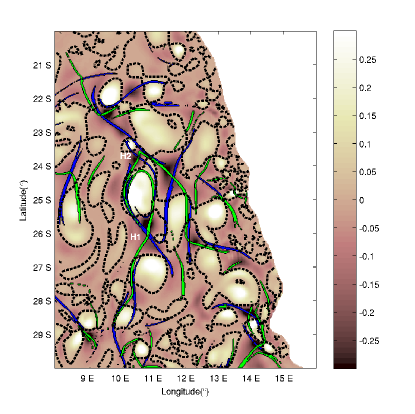
Figure 6: $Q$-criterium map at 200 m depth together with patches of backward (blue) and forward (green) FSLE values. Black dashed lines have $Q=0$. FSLE patches contain the highest 60% of FSLE values. Colorbar values are $Q\times 10^{10}\>s^{-2}$.The eddy we study is the clear region in between points H1 and H2.

Let us move to the Lagrangian description of eddies, which is much in the spirit of our study, and will allow us to study particle transport: eddies can be defined as the region bounded by intersecting or tangent repelling and attracting LCS (Branicki and Kirwan, 2010; Branicki et al., 2011). Using this criterion, and first looking at the surface located at 200 m depth, we see in Fig. 6 that certainly the Eulerian eddy seems to be located inside the area defined by several intersections and tangencies of the LCS. This eddy has an approximate diameter of $100$ km. In the south-north direction there are two intersections that appear to be hyperbolic points (H1 and H2 in figure 6). In the West-East direction, the eddy is closed by a tangency at the western boundary, and a intersection of lines at the eastern boundary. The eddy core is devoid of high FSLE lines, indicating that weak stirring occurs inside (d’Ovidio et al., 2004). As additional Eulerian properties, we note that near or at the intersections H1 and H2 the $Q$-criterium indicates straining motions. In the case of H2, figure 5 (right panel) indicates high shear up to 200 m depth. The fact that the hyperbolic regions H1 and H2 lie in strain dominated regions of the flow ($Q<0$) highlights the connection between hyperbolic particle behavior and instantaneous hyperbolic regions of the flow. The ridges of the FSLE field, however, do not remain in the negative $Q$ regions but cross into rotation dominated regions with $Q>0$. This indicates that there are some differences between the Eulerian view (Q) and the Lagrangian view (FSLE). It is the latter that can be understood in terms of particle behaviour as limiting regions of initial conditions (particles) that stay away from hyperbolic regions for long enough time (Haller and Yuan, 2000).

In 3d, the eddy is also surrounded by a set of attracting and repelling LCS (figure 7), calculated as explained in Subsection 2.3. The lines identified in figure 6 are now seen to belong to the vertical of these surfaces.

Figure 7: 3d LCSs around the mesoscale eddy at day $1$ of the $30$ day FSLE calculation period. Green: repelling LCS; Blue: attracting LCS.

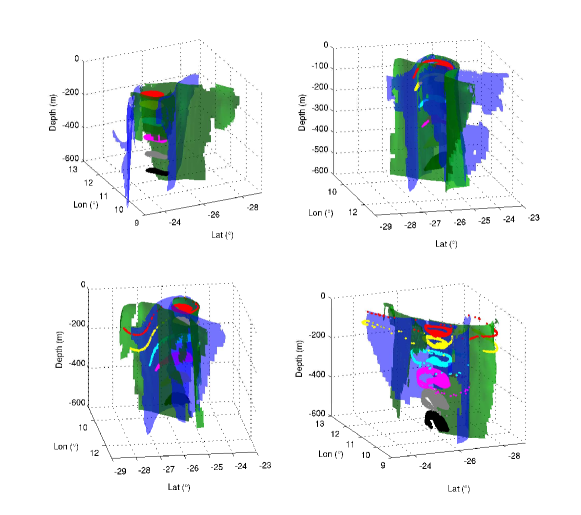
Figure 8: Three dimensional view of the evolution of elliptic patches released at different depths inside of the eddy at day 1 of the 30 day FSLE calculaton period. Top left: day 3; Top right: day 13; Bottom left: day 19: Bottom right: day 29. Red: 40 m; Yellow: 100 m; Cyan: 200 m; Magenta: 300 m; Grey: 400 m; Black: 500 m. Attracting LCS are shaded in blue while repelling LCS are shaded in green.

Note that the vertical extent of these surfaces is in part determined by the strength parameter used in the LCS extraction process, so their true vertical extension is not clear from the results presented here. On the south, the closure of the Lagrangian eddy boundary extends down to the maximum depth of the calculation domain, but moving northward it is seen that the LCS shorten their depth. Probably this does not mean that the eddy is shallower in the North, but rather that the LCS are losing strength (lower $|\alpha_{3}|$) and portions of it are filtered out by the extraction process. In any case, it is seen that as in two-dimensional calculations, the LCS delimiting the eddy do not perfectly coincide with its Eulerian boundary (Joseph and Legras, 2002), and we expect the Lagrangian view to be more relevant to address transport questions.

In the next paragraphs we analyze the fluid transport across the eddy boundary. Some previous results for Lagrangian eddies were obtained by Branicki and Kirwan (2010) and Branicki et al. (2011). Applying the methodology of lobe dynamics and the turnstile mechanism to eddies pinched off from the Loop Current, Branicki and Kirwan (2010) observed a net fluid entrainment near the base of the eddy, and net detrainment near the surface, being fluid transport in and out of the eddy essentially confined to the boundary region. Let us see what happens in our setting.

We consider six sets of $1000$ particles each, that were released at day $1$ of the FSLE calculation period, and their trajectories integrated by a fourth-order Runge-Kutta method with a integration time step of $6$ hours. The sets of particles were released at depths of $50$, $100$, $200$, $300$, $400$ and $500$ m. In figure 8 we plot the particle sets together with the Lagrangian boundaries of the mesoscale eddy viewed in 3d. A top view is shown in figure 9. As expected, vertical displacements are small.

At day $3$ (top left panel of figures 8 and 9) it can be seen that there is a differential rotation (generally cyclonic, i.e. clockwise) between the sets of particles at different depths. The shallower sets rotate faster than the deeper ones. This differential rotation of the fluid particles could be viewed, in a Lagrangian perspective, as the fact that the attracting and repelling strength of the LCS that limit the eddy varies with depth. Note that the six sets of particles are released at the same time and at the same horizontal positions, and thereby their different behavior is due to the variations of the LCS properties along depth.

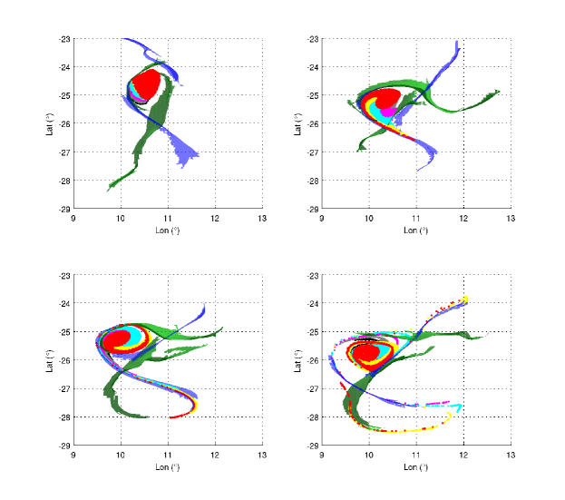
Figure 9: Top view of the evolution of particle patches and LCSs shown in Fig. 8. Top left: day 3; Top right: day 13; Bottom left: day 19: Bottom right: day 29. Colors as in figure 8.

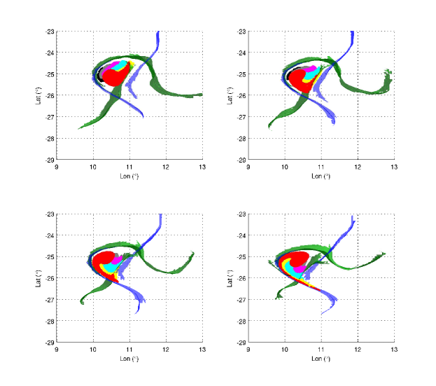
Figure 10: Top view of the initial stages of evolution of the particle patches and LCSs of Figs. 8 and 9. Top left: day 7; Top right: day 9; Bottom left: day 11: Bottom right: day 13. Colors as in figure 8.

At day $13$ the vortex starts to expel material trough filamentation (Figs.8 and 9, top right panels). A fraction of the particles approach the southern boundaries of the eddy from the northeast. Those to the west of the repelling LCS (green) turn west and recirculate inside the eddy along the southern attracting LCS (blue). Particles to the east of the repelling LCS turn east and leave the eddy forming a filament aligned with an attracting (blue) LCS. At longer times trajectories in the south of the eddy are influenced by additional structures associated to a different southern eddy. At day 29 (bottom right panels) the same process is seen to have occurred in the northern boundary, with a filament of particles leaving the eddy along the northern attracting (blue) LCS. The filamentation seems to begin earlier at shallower waters than at deeper ones since the length of the expelled filament diminishes with depth. However all of the expelled filaments follow the same attracting LCS. Figure 10 shows the stages previous to filamentation in which the LCS structure, their tangencies and crossings, and the paths of the particle patches are more clearly seen. Note that the LCS do not form fully closed structures and the particles escape the eddy through their openings. The images suggest lobe-dynamics processes, but much higher precision in the LCS extraction would be needed to really see such details.

This filamentation event seems to be the only responsible for transport of material outside of the eddy, since the rest of the particles remained inside the eddy boundaries. To get a rough estimate of the amount of matter expelled in the filamentation process we tracked the percentage of particles leaving a circle of diameter 200 km centered on the eddy center. In Fig. 11 the time evolution of this percentage is shown for the particle sets released at different depths. The onset of filamentation is clearly visible around days 9-12 as a sudden increase in the percentage of particles leaving the eddy. The percentage is maximum for the particles located at 100 m depth and decreases as the depth increases. At 400 and 500 m depth there are no particles leaving the circle. There is a clear lag between the onset of filamentation between the different depths: the onset is simultaneous for the 40 m and 100 m depths but occurs later for larger depths.

4 Discussion.

The spatial average of FSLEs defines a measure of stirring and thus of horizontal mixing between the scales used for its computation. The larger the average, the larger the mixing activity (d’Ovidio et al., 2004). The general trend in the vertical profiles of the average FSLE (Fig. 3) shows a reduction of mesoscale mixing with depth. There is however a rather interesting peak in this average profile occurring at 100 m, i.e. close to the thermocline. It could be related to submesoscale processes that occur alongside the mesoscale ones. Submesoscale is associated to filamentation (the thickness of filaments is of the order of $10$ km or less), and we have seen that the filamentation and the associated transport intensity (Fig. 11) is higher at $100$ m depth. It is not clear at the moment what is the precise mechanism responsible for this increased activity at around 100 m depth (perhaps associated to instabilities in the mixed layer), but we note that the intensity of shearing motions (see the $Q$ plots in 5) is higher in the top 200 meters. Less intense filamentation could be caused by reduction of shear in depths larger than these values.

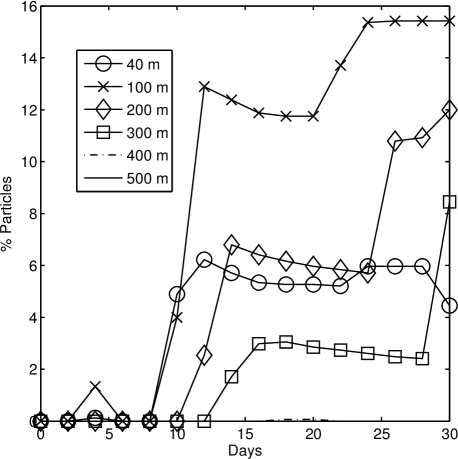
Figure 11: Percentage of particles outside a $200$ km diameter circle centered at the eddy center, as a function of time.

From an Eulerian perspective, it is thought that vortex filamentation occurs when the potential vorticity (PV) gradient aligns itself with the compressional axis of the velocity field, in strain coordinates (Louazel and Hua (2004);Lapeyre et al. (1999)). This alignment is accompanied by exponential growth of the PV gradient magnitude. The fact that the filamentation occurs along the attracting LCS seems to indicate that this exponential growth of the PV gradient magnitude occurs across the attracting LCS.

In the specific spatiotemporal area we have studied, and in particular, for the eddy on which we focussed our analysis, we have confirmed that the structure of the LCSs is “curtain-like”, so that the strongest attracting and repelling structures are quasivertical surfaces. Their vertical extension would depend of the physical transport properties, but it is also altered by the particular threshold parameter selected to extract the LCSs. These observations imply that transport and stirring occurs mainly on the horizontal, which is a reasonable result considering the disparity between horizontal and vertical velocities in the ocean, and its stratification. However, we should mention that our results are not fully generalizable to all ocean situations, and that any ocean area or oceanic event should be studied in particular to reveal the shape of the associated 3d LCS.

Some comments follow about the nature of vertical transport structures. FSLEs are suited to the identification of hyperbolic structures (structures that exhibit high rates of transversal stretching or compression in their vicinity). The question is if one can expect that structures responsible for vertical transport will also exhibit substantial (vertical) stretching. This is not so clear in the ocean for the reasons already indicated. If one considers the case (relevant to our work) of purely isopycnal flow, then strong vertical stretching would be associated with a rapid divergence of isopycnic surfaces. In the case of coastal upwelling, for instance, the lifted isopycnic surfaces move vertically in a coherent fashion, so one should not expect strong vertical divergence of particles flowing along neighbouring isopycnic surfaces. This is just an example of the fact that it is possible that coherent vertical motions do not imply the presence of hyperbolic coherent structures such as those the FSLE may indicate.

Another possible limitation worth mentioning is the velocity field resolution and its relation to the intensity of the vertical velocity. It is accepted that in fronts or in the eddy periphery, vertical velocities are significantly greater than, for instance, in the eddy interior. These zones of enhanced vertical transport correspond to submesoscale features that were not adequately captured in the velocity field used in this work due to its coarse resolution, since submesoscale studies usually have resolutions $<10$ km (the literature on this subject is quite large, so we refer the reader to Klein and Lapeyre (2009) and Lévy (2008) ).

In any case, a most important point for the LCS we have computed is that in 3d, as in 2d, they act as pathways and barriers to transport, so that they provide a skeleton organizing the transport processes.

5 Conclusions

Three dimensional Lagrangian Coherent Structures were used to study stirring processes leading to dispersion and mixing at the mesoscale in the Benguela ocean region. We have computed 3d Finite Size Lyapunov Exponent fields, and LCSs were identified with the ridges these fields. LCSs appear as quasivertical surfaces, so that horizontal cuts of the FSLE fields gives already a quite accurate vision of the 3d FSLE distribution. These quasivertical surfaces appear to be coincident with the maximal lines of the FSLE field (see fig. 3) so that surface FSLE maps could be indicative of the position of 3d LCS, as long as the vertical shear of the velocity does not result in a significant deviation of the LCS with respect to the vertical. Average FSLE values generally decrease with depth, but we find a local maximum, and thus enhanced stretching and dispersion, at about 100 m depth.

We have also analyzed a prominent cyclonic eddy, pinched off the upwelling front and study the filamentation dynamics in 3d. Lagrangian boundaries of the eddy were made of intersections and tangencies of attracting and repelling LCS that apparently emanating from two hyperbolic locations North and South of the eddy. The LCS are seen to provide pathways and barriers organizing the transport processes and geometry. This pattern extends down up to the maximum depth were we calculated the FSLE fields ($\sim 600$ m), but the exact shape of the boundary is difficult to determine due to the decrease in ridge strength with depth. This caused some parts of the LCS not to be extracted. The inclusion of a variable strength parameter in the extraction process is an important step to be included in the future.

The filamentation dynamics, and thus the transport out of the eddy, showed time lags with increasing depth. This arises from the vertical variation of the flow field. However the filamentation occurred along all depths, indicating that in reality vertical sheets of material are expelled from these eddies.

Many more additional studies are needed to further clarify the details of the geometry of the LCSs, their relationships with finite-time hyperbolic manifolds and three dimensional lobe dynamics, and specially their interplay with mesoscale and submesoscale transport and mixing processes.

References

- Amante and Eakins (2009) Amante, C., Eakins, B.W., 2009. ETOPO1 1 Arc-Minute Global Relief Model: Procedures, Data Sources and Analysis. NOAA Technical Memorandum NESDIS NGDC-24.
- Artale et al. (1997) Artale, V., Boffetta, G., Celani, A., Cencini, M., Vulpiani, A., 1997. Dispersion of passive tracers in closed basins: Beyond the diffusion coefficient. Phys. Fluids 9, 3162–3171.
- Aurell et al. (1997) Aurell, E., Boffetta, G., Crisanti, A., Paladin, G., Vulpiani, A., 1997. Predictability in the large: an extension of the Lyapunov exponent. J. Phys. A 30, 1–26.
- Beron-Vera et al. (2008) Beron-Vera, F., Olascoaga, M., Goni, G., 2008. Oceanic mesoscale eddies as revealed by Lagrangian coherent structures. Geophys. Res. Lett 35, L12603.
- Boffetta et al. (2001) Boffetta, G., Lacorata, G., Redaelli, G., Vulpiani, A., 2001. Detecting barriers to transport: a review of different techniques. Physica D 159, 58–70.
- Branicki and Kirwan (2010) Branicki, M., Kirwan, A., 2010. Stirring: The Eckart paradigm revisited. Int. J. Eng. Sci. 48, 1027–1042.
- Branicki and Malek-Madani (2010) Branicki, M., Malek-Madani, R., 2010. Lagrangian structure of flows in the Chesapeake Bay: challenges and perspectives on the analysis of estuarine flows. Nonlinear Processes in Geophysics 17, 149–168.
- Branicki et al. (2011) Branicki, M., Mancho, A.M., Wiggins, S., 2011. A Lagrangian description of transport associated with a front-eddy interaction: Application to data from the North-Western Mediterranean sea. Physica D: Nonlinear Phenomena 240, 282 – 304.
- Branicki and Wiggins (2009) Branicki, M., Wiggins, S., 2009. Finite-time Lagrangian transport analysis: Stable and unstable manifolds of hyperbolic trajectories and finite-time Lyapunov exponents. Nonlinear Processes in Geophysics 17, 1–36.
- Byrne et al. (1995) Byrne, D.A., Gordon, A.L., Haxby, W.F., 1995. Agulhas eddies: A synoptic view using Geosat ERM data. J. Phys. Oceanogr. 25, 902–917.
- Doglioli et al. (2007) Doglioli, A., Blanke, B., Speich, S., Lapeyre, G., 2007. Tracking coherent structures in a regional ocean model with wavelet analysis: Application to cape basin eddies. Journal of Geophysical Research C: Oceans 112, C05043.
- d’Ovidio et al. (2004) d’Ovidio, F., Fernández, V., Hernández-García, E., López, C., 2004. Mixing structures in the Mediterranean sea from Finite-Size Lyapunov Exponents. Geophys. Res. Lett. 31, L17203.
- d’Ovidio et al. (2009) d’Ovidio, F., Isern, J., López, C., Hernández-García, E., García-Ladona, E., 2009. Comparison between Eulerian diagnostics and Finite-Size Lyapunov Exponents computed from Altimetry in the Algerian basin. Deep-Sea Res. I 56, 15–31.
- Eberly et al. (1994) Eberly, D., Gardner, R., Morse, B., Pizer, S., Scharlach, C., 1994. Ridges for image analysis. Journal of Mathematical Imaging and Vision 4, 353–373.
- Elhmaïdi et al. (1993) Elhmaïdi, D., Provenzale, A., Babiano, A., 1993. Elementary topology of two-dimensional turbulence from a Lagrangian viewpoint and single-particle dispersion. J. Fluid Mech. 257, 533–558.
- Haller (2000) Haller, G., 2000. Finding finite-time invariant manifolds in two-dimensional velocity fields. Chaos 10(1), 99–108.
- Haller (2001) Haller, G., 2001. Distinguished material surfaces and coherent structure in three-dimensional fluid flows. Physica D 149, 248–277.
- Haller (2002) Haller, G., 2002. Lagrangian coherent structures from approximate velocity data. Phys. Fluids A14, 1851–1861.
- Haller (2011) Haller, G., 2011. A variational theory of hyperbolic lagrangian coherent structures. Physica D 240, 574–598.
- Haller and Yuan (2000) Haller, G., Yuan, G., 2000. Lagrangian coherent structures and mixing in two-dimensional turbulence. Physica D 147, 352–370.
- Haza et al. (2010) Haza, A., Özgökmen, T., Griffa, A., Molcard, A., Poulain, P.M., Peggion, G., 2010. Transport properties in small-scale coastal flows: relative dispersion from VHF radar measurements in the Gulf of La Spezia. Ocean Dynamics 60, 861–882.
- Haza et al. (2008) Haza, A.C., Poje, A.C., Özgökmen, T.M., Martin, P., 2008. Relative dispersion from a high-resolution coastal model of the Adriatic Sea. Ocean Modell. 22, 48–65.
- Hernandez-Carrasco et al. (2011) Hernandez-Carrasco, I., López, C., Hernández-García, E., Turiel, A., 2011. How reliable are finite-size Lyapunov exponents for the assessment of ocean dynamics? Ocean Modell. 36, 208–218.
- Hunt et al. (1988) Hunt, J.C.R., Wray, A.A., Moin, P., 1988. Eddies, Streams and Convergence Zones in Turbulent Flows. Technical Report CTR-S88. Center for Turbulence Research, Standford University. 193–208.
- Jeong and Hussain (1995) Jeong, J., Hussain, F., 1995. On the identification of a vortex. J. Fluid Mech. 285, 69–94.
- Joseph and Legras (2002) Joseph, B., Legras, B., 2002. Relation between kinematic boundaries, stirring, and barriers for the Antartic polar vortex. J. Atm. Sci. 59, 1198–1212.
- Klein and Lapeyre (2009) Klein, P., Lapeyre, G., 2009. The oceanic vertical pump induced by mesoscale and submesoscale turbulence. Ann. Rev. Mar. Sci. 1, 351–375.
- Lacasce (2008) Lacasce, J., 2008. Statistics from Lagrangian observations. Progress in oceanography 77, 1–29.
- Lapeyre et al. (1999) Lapeyre, G., Klein, P., Hua, B., 1999. Does the tracer gradient vector align with strain eigenvectors in 2d turbulence? Phys. Fluids 11, 3729–3737.
- Le Vu et al. (2011) Le Vu, B., Gutknecht, E., Machu, E., Dadou, I., Veitch, J., Sudre, J., Paulmier, A., Garçon, V., 2011. Processes maintaining the OMZ of the benguela upwelling systemusing an eddy resolving model. submitted to JMR .
- Lehahn et al. (2011) Lehahn, Y., d’Ovidio, F., Lévy, M., Amitai, Y., Heifetz, E., 2011. Long range transport of a quasi isolated chlorophyll patch by an Agulhas ring. Geophys. Res. Lett. 38, L16610.
- Lekien et al. (2007) Lekien, F., Shadden, S.C., Marsden, J.E., 2007. Lagrangian coherent structures in n-dimensional systems. J. Math. Phys. 48, 065404.
- Louazel and Hua (2004) Louazel, S., Hua, B.L., 2004. Vortex erosion in a shallow-water model. Physics of Fluids 16, 3079–3085.
- Lévy (2008) Lévy, M., 2008. The modulation of biological production by oceanic mesoscale turbulence, in: Weiss, J., Provenzale, A. (Eds.), Transport and Mixing in Geophysical Flows. Springer Berlin / Heidelberg. volume 744 of Lecture Notes in Physics, pp. 219–261.
- Mahadevan (2006) Mahadevan, A., 2006. Modeling vertical motion at ocean fronts: Are nonhydrostatic effects relevant at submesoscales? Ocean Modelling 14, 222 – 240.
- Mancho et al. (2006) Mancho, A.M., Small, D., Wiggins, S., 2006. A tutorial on dynamical systems concepts applied to Lagrangian transport in ocean flows defined as finite time data sets: theoretical and computational issues. Phys. Rep. 437, 55–124.
- Mariano et al. (2002) Mariano, A.J., Griffa, A., Özgökmen, T., Zambianchi, E., 2002. Lagrangian analysis and predictability of coastal and ocean dynamics 2000. J. Atmos. Oceanic Technol. 19, 1114–1126.
- McGillicuddy et al. (1998) McGillicuddy, D.J., Robinson, A.R., Siegel, D.A., Jannasch, H.W., Johnson, R., Dickey, T.D., McNeil, J., Michaels, A.F., Knap, A.H., 1998. Influence of mesoscale eddies on new production in the Sargasso sea. Nature 394, 263–266.
- Molcard et al. (2006) Molcard, A., Poje, A., Özgökmen, T., 2006. Directed drifter launch strategies for Lagrangian data assimilation using hyperbolic trajectories. Ocean Modell. 12, 268–289.
- Okubo (1970) Okubo, A., 1970. Horitzontal dispersion of floatable particles in the vicinity of velocity singularities such as convergences. Deep-Sea Res. I 17, 445–454.
- Oschlies and Garçon (1998) Oschlies, A., Garçon, V., 1998. Eddy-induced enhancement of primary productivity in a model of the North Atlantic ocean. Nature 394, 266–269.
- Özgökmen et al. (2011) Özgökmen, T.M., Poje, A.C., Fischer, P.F., Haza, A.C., 2011. Large eddy simulations of mixed layer instabilities and sampling strategies. Ocean Modell. 39, 311–331.
- Pauly and Christensen (1995) Pauly, D., Christensen, V., 1995. Primary production required to sustain global fisheries 374, 255–257.
- Poje et al. (2010) Poje, A.C., Haza, A.C., Özgökmen, T.M., Magaldi, M.G., Garraffo, Z.D., 2010. Resolution dependent relative dispersion statistics in a hierarchy of ocean models. Ocean Modell. 31, 36–50.
- Pouransari et al. (2010) Pouransari, Z., Speetjens, M., Clercx, H., 2010. Formation of coherent structures by fluid inertia in three-dimensional laminar flows. J. Fluid Mech. 654, 5–34.
- Provenzale (1999) Provenzale, A., 1999. Transport by coherent barotropic vortices. Annu. Rev. Fluid Mech. 31, 55–93.
- Rossi et al. (2008) Rossi, V., López, C., Sudre, J., Hernández-García, E., Garçon, V., 2008. Comparative study of mixing and biological activity of the Benguela and Canary upwelling systems. Geophys. Res. Lett. 35, L11602.
- Rubio et al. (2009) Rubio, A., Blanke, B., Speich, S., Grima, N., Roy, C., 2009. Mesoscale eddy activity in the southern Benguela upwelling system from satellite altimetry and model data. Progress In Oceanography 83, 288 – 295.
- Sadlo and Peikert (2007) Sadlo, F., Peikert, R., 2007. Efficient visualization of Lagrangian Coherent Structures by filtered AMR ridge extraction. IEEE Transactions on Visualization and Computer Graphics 13, 1456–1463.
- Schultz et al. (2010) Schultz, T., Theisel, H., Seidel, H.P., 2010. Crease surfaces: From theory to extraction and application to diffusion tensor MRI. IEEE Transactions on Visualization and Computer Graphics 16, 109–119.
- Shadden et al. (2005) Shadden, S.C., Lekien, F., Marsden, J.E., 2005. Definition and properties of Lagrangian coherent structures from finite-time Lyapunov exponents in two-dimensional aperiodic fows. Physica D. 212, 271–304.
- Shchepetkin and McWilliams (2003) Shchepetkin, A.F., McWilliams, J.C., 2003. A method for computing horizontal pressure-gradient force in an oceanic model with a nonaligned vertical coordinate. J. Geophys. Res. 108, 3090.
- Shchepetkin and McWilliams (2005) Shchepetkin, A.F., McWilliams, J.C., 2005. The regional ocean modeling system: A split-explicit, free-surface, topography following coordinates ocean model. Ocean Modell. 9, 347–404.
- Tallapragada et al. (2011) Tallapragada, P., Ross, S.D., Schmale III, D.G., 2011. Lagrangian coherent structures are associated with fluctuations in airborne microbial populations. Chaos 21, 033122.
- Tang et al. (2011) Tang, W., Chan, P.W., Haller, G., 2011. Lagrangian coherent structure analysis of terminal winds detected by lidar. part i: Turbulence structures. Journal of Applied Meteorology and Climatology 50, 325–338.
- Thomas et al. (2008) Thomas, L., Tandon, A., Mahadevan, A., 2008. Submesoscale ocean processes and dynamics, in: Hecht, M., Hasume, H. (Eds.), Ocean Modeling in an Eddying Regime, Geophysical Monograph 177, American Geophysical Union, Washington D.C.. pp. 17–38.
- du Toit and Marsden (2010) du Toit, P., Marsden, J., 2010. Horseshoes in hurricanes. Journal of Fixed Point Theory and Applications 7, 351–384. 10.1007/s11784-010-0028-6.
- Waugh et al. (2006) Waugh, D.W., Abraham, E.R., Bowen, M.M., 2006. Spatial variations of stirring in the surface ocean: A case of study of the Tasman sea. J. Phys. Oceanogr. 36, 526–542.
- Weiss (1991) Weiss, J., 1991. The dynamics of enstrophy transfer in two-dimensional hydrodynamics. Physica D 48, 273–294.
- Yuan et al. (1994) Yuan, K.Y., Huang, Y.S., Yang, H.T., Pian, T.H.H., 1994. The inverse mapping and distortion measures for 8-node hexahedral isoparametric elements. Computational Mechanics 14, 189–199.