THE NUMERICAL GENERALIZED LEAST-SQUARES ESTIMATOR OF AN UNKNOWN CONSTANT MEAN OF RANDOM FIELD

Abstract.

We constraint on computer the best linear unbiased generalized statistics of random field for the best linear unbiased generalized statistics of an unknown constant mean of random field and derive the numerical generalized least-squares estimator of an unknown constant mean of random field. We derive the third constraint of spatial statistics and show that the classic generalized least-squares estimator of an unknown constant mean of the field is only an asymptotic disjunction of the numerical one.

1. The best linear unbiased generalized statistics

Remark. To simplify notation we use Einstein summation convention then

$$\sum_{i=1}^{n}\omega^{i}_{j}\rho_{ij}=\omega^{i}_{j}\rho_{ij}=w^{\prime}r\,$$

where

$$\begin{array}[]{cccccccccc}w&=&\underbrace{\left[\begin{array}[]{c}\omega_{j}^{\it 1}\\ \vdots\\ \omega_{j}^{\it n}\\ \end{array}\right]}_{n\times 1}\ ,&r&=&\underbrace{\left[\begin{array}[]{c}\rho_{\it 1j}\\ \vdots\\ \rho_{\it nj}\\ \end{array}\right]}_{n\times 1}\end{array}$$

are given vectors and

$$\sum_{i=1}^{n}\omega^{i}_{j}\sum_{l=1}^{n}\rho_{il}\omega^{l}_{j}=\omega^{i}_{j}\rho_{il}\omega^{l}_{j}=w^{\prime}\Lambda w\ ,$$

where

$$\begin{array}[]{ccccc}\Lambda&=&{\underbrace{\left[\begin{array}[]{ccc}\rho_{\it 11}&\ldots&\rho_{\it 1n}\\ \vdots&\ddots&\vdots\\ \rho_{\it n1}&\ldots&\rho_{\it nn}\\ \end{array}\right]}_{n\times n}}\end{array}$$

is given matrix.

Let us consider the random field $V_{j};~{}j\in{\mathbb{N}}_{1}$ with an unknown constant mean $m$ and variance $\sigma^{2}$ its estimation statistics $\hat{V}_{j}$ and the variance of the difference $R_{j}=V_{j}-\hat{V}_{j}$, where $E\{V_{j}\}=E\{\hat{V}_{j}\}=m$, as covariance

$$\begin{array}[]{ccc}D^{2}\{V_{j}-\hat{V}_{j}\}&=&Cov\{(V_{j}-\hat{V}_{j})(V_{j}-\hat{V}_{j})\}\\ &=&Cov\{V_{j}V_{j}\}-Cov\{V_{j}\hat{V}_{j}\}-Cov\{\hat{V}_{j}V_{j}\}+Cov\{\hat{V}_{j}\hat{V}_{j}\}\\ &=&Cov\{V_{j}V_{j}\}-2Cov\{\hat{V}_{j}V_{j}\}+Cov\{\hat{V}_{j}\hat{V}_{j}\}\end{array}$$

and the linear estimation statistics (weighted variable) $\hat{V}_{j}=\sum_{i=1}^{n}\omega^{i}_{j}V_{i}=\omega^{i}_{j}V_{i};~{}j\subset i=1,\ldots,n$ at $j\geq n+1$ then

(1) $$D^{2}\{R_{j}\} = Cov\{V_{j}V_{j}\}-2Cov\{\hat{V}_{j}V_{j}\}+Cov\{\hat{V}_{j}\hat{V}_{j}\}$$

$$= Var\{V_{j}\}-2Cov\{\sum_{i}\omega_{j}^{i}V_{i}V_{j}\}+Cov\{(\sum_{i}\omega^{i}_{j}V_{i})(\sum_{i}\omega^{i}_{j}V_{i})\}$$

$$= \sigma^{2}-2\sum_{i}\omega^{i}_{j}Cov\{V_{i}V_{j}\}+\sum_{i}\sum_{l}\omega^{i}_{j}\omega^{l}_{j}Cov\{V_{i}V_{l}\}$$

$$= \sigma^{2}-2\sigma^{2}|\omega^{i}_{j}\rho_{ij}|+\sigma^{2}|\omega^{i}_{j}\rho_{il}\omega^{l}_{j}|$$

$$= \sigma^{2}\pm 2\sigma^{2}\omega^{i}_{j}\rho_{ij}\mp\sigma^{2}\omega^{i}_{j}\rho_{il}\omega^{l}_{j}\ ,$$

where $\rho_{ij};~{}i=1,\ldots,n$ is given vector of correlations and $\rho_{il};~{}i,l=1,\ldots,n$ is given (symmetric) matrix of correlations (see Appendix A).
The unbiasedness constraint (the first constraint on the estimation statistics)

$$E\{R_{j}\}=E\{V_{j}-\hat{V}_{j}\}=E\{V_{j}\}-E\{\hat{V}_{j}\}=E\{V_{j}\}-E\{\omega^{i}_{j}V_{i}\}=m-m\sum_{i=1}^{n}\omega^{i}_{j}=0$$

equal to

(2) $$\sum_{i=1}^{n}\omega^{i}_{j}=f_{\it 1i}\omega^{i}_{j}=\omega^{i}_{j}f_{\it i1}=1$$

gives the first equation

$$\begin{array}[]{ccccccccc}{\underbrace{\left[\begin{array}[]{ccc}1&\ldots&1\end{array}\right]}_{1\times n}}&\cdot&\underbrace{\left[\begin{array}[]{c}\omega^{1}_{j}\\ \vdots\\ \omega^{n}_{j}\\ \end{array}\right]}_{n\times 1}&=&{\underbrace{\left[\begin{array}[]{ccc}\omega^{1}_{j}&\ldots&\omega^{n}_{j}\end{array}\right]}_{1\times n}}&\cdot&\underbrace{\left[\begin{array}[]{c}1\\ \vdots\\ 1\\ \end{array}\right]}_{n\times 1}&=&1\ .\end{array}$$

The minimization constraint (the second constraint on the estimation statistics – the statistics is the best)

(3) $$\frac{\partial D^{2}\{R_{j}\}}{\partial\omega^{i}_{j}}=\pm 2\sigma^{2}\rho_{ij}\mp 2\sigma^{2}\rho_{il}\omega^{l}_{j}\mp 2\sigma^{2}f_{\it i1}\mu_{j}^{\it 1}=0\ ,$$

where (1)

$$D^{2}\{R_{j}\}=\sigma^{2}\pm 2\sigma^{2}\omega^{i}_{j}\rho_{ij}\mp\sigma^{2}\omega^{i}_{j}\rho_{il}\omega^{l}_{j}\mp 2\sigma^{2}\underbrace{\left(\omega^{i}_{j}f_{\it i1}-1\right)}_{0}\mu_{j}^{\it 1}\ ,$$

produces $n$ equations in $n+1$ unknowns the kriging weights $\omega_{j}^{i}$ and a Lagrange parameter $\mu^{\it 1}_{j}$

$$\begin{array}[]{cccccl}{\underbrace{\left[\begin{array}[]{cccc}\rho_{\it 11}&\ldots&\rho_{\it 1n}&1\\ \vdots&\ddots&\vdots&\vdots\\ \rho_{\it n1}&\ldots&\rho_{\it nn}&1\\ \end{array}\right]}_{n\times(n+1)}}&\cdot&\underbrace{\left[\begin{array}[]{c}\omega_{j}^{\it 1}\\ \vdots\\ \omega_{j}^{\it n}\\ \mu_{j}^{\it 1}\\ \end{array}\right]}_{(n+1)\times 1}&=&\underbrace{\left[\begin{array}[]{c}\rho_{\it 1j}\\ \vdots\\ \rho_{\it nj}\\ \end{array}\right]}_{n\times 1}\end{array}$$

this system of equations if multiplied by $\omega^{i}_{j}$

$$\omega^{i}_{j}\rho_{il}\omega^{l}_{j}+\underbrace{\omega^{i}_{j}f_{\it i1}}_{1}\mu^{\it 1}_{j}=\omega^{i}_{j}\rho_{ij}\ ,$$

and substituted into

$$\begin{array}[]{ccc}D^{2}\{R_{j}\}&=&E\{[V_{j}-\hat{V}_{j}]^{2}\}-\underbrace{E^{2}\{V_{j}-\hat{V}_{j}\}}_{0}\\ &=&E\{[(V_{j}-m)-(\hat{V}_{j}-m)]^{2}\}\\ &=&E\{[V_{j}-m]^{2}\}-2(E\{V_{j}\hat{V}_{j}\}-m^{2})+E\{[\hat{V}_{j}-m]^{2}\}\\ &=&\sigma^{2}-2\sigma^{2}|\omega^{i}_{j}\rho_{ij}|+\sigma^{2}|\omega^{i}_{j}\rho_{il}\omega^{l}_{j}|\\ &=&\sigma^{2}\pm 2\sigma^{2}\omega^{i}_{j}\rho_{ij}\mp\sigma^{2}\omega^{i}_{j}\rho_{il}\omega^{l}_{j}\end{array}$$

since variance of the (estimation) statistics is minimized

(4) $$E\{[\hat{V}_{j}-m]^{2}\} = Cov\{(\omega^{i}_{j}V_{i})(\omega^{i}_{j}V_{i})\}$$

$$= \sum_{i}\sum_{l}\omega^{i}_{j}\omega^{l}_{j}Cov\{V_{i}V_{l}\}$$

$$= \sigma^{2}|\omega^{i}_{j}\rho_{il}\omega^{l}_{j}|$$

$$= \mp\sigma^{2}\omega^{i}_{j}\rho_{il}\omega^{l}_{j}$$

$$= \mp\sigma^{2}(\omega^{i}_{j}\rho_{ij}-\mu_{j}^{\it 1})$$

gives

(5) $$D^{2}\{R_{j}\}=E\{[V_{j}-\hat{V}_{j}]^{2}\}=E\{[(V_{j}-m)-(\hat{V}_{j}-m)]^{2}\}=\sigma^{2}(1\pm(\omega^{i}_{j}\rho_{ij}+\mu^{\it 1}_{j}))$$

the constraints (2) and (3) produce $n+1$ equations in $n+1$ unknowns

(6) $$\begin{array}[]{cccccl}{\underbrace{\left[\begin{array}[]{cccc}\rho_{\it 11}&\ldots&\rho_{\it 1n}&1\\ \vdots&\ddots&\vdots&\vdots\\ \rho_{\it n1}&\ldots&\rho_{\it nn}&1\\ 1&\ldots&1&0\\ \end{array}\right]}_{(n+1)\times(n+1)}}&\cdot&\underbrace{\left[\begin{array}[]{c}\omega_{j}^{\it 1}\\ \vdots\\ \omega_{j}^{\it n}\\ \mu^{\it 1}_{j}\\ \end{array}\right]}_{(n+1)\times 1}&=&\underbrace{\left[\begin{array}[]{c}\rho_{\it 1j}\\ \vdots\\ \rho_{\it nj}\\ 1\\ \end{array}\right]}_{(n+1)\times 1}\ .\end{array}$$

2. The classic best linear unbiased generalized statistics of an unknown constant mean of the field

Remark. When we consider an independent set of the random variables $V_{i};~{}i=1,\ldots,n$ with an unknown constant mean $m$ and variance $\sigma^{2}$ the best linear unbiased ordinary (estimation) statistics $\hat{V}_{j}=\omega^{i}_{j}V_{i}$ of the field $V_{j};~{}j\subset i=1,\ldots,n$ has the asymptotic property

(7) $$\lim_{n\rightarrow\infty}E\{[\omega^{i}_{j}V_{i}-m]^{2}\}=0$$

whilst for spatial dependence between random variables (the best linear unbiased generalized statistics) we get (see Appendix B)

(8) $$\lim_{n\rightarrow\infty}\lim_{j\rightarrow\infty}E\{[\omega^{i}_{j}V_{i}-m]^{2}\}=0\ .$$

Due to different asymptotic limits between (7) and (8) the ordinary least-squares estimator of an unknown constant mean $m$ of the field, the best linear unbiased estimator of an unknown constant mean $m$ of the field, can not be so easy generalized (like it was in past).

Let us constraint the best linear unbiased generalized (estimation) statistics $\hat{V}_{j}=\omega^{i}_{j}V_{i}$ of the random field $V_{j};~{}j\subset i=1,\ldots,n$, when for finite $n$ and $j\rightarrow\infty$ the vector of correlations simplifies to

(9) $$\underbrace{\left[\begin{array}[]{c}\rho_{1j}\\ \vdots\\ \rho_{nj}\\ \end{array}\right]}_{n\times 1}=\xi\underbrace{\left[\begin{array}[]{c}1\\ \vdots\\ 1\\ \end{array}\right]}_{n\times 1}\qquad\xi\rightarrow 0^{-}~{}(\mbox{or}~{}\xi\rightarrow 0^{+})$$

then from (2)

(10) $$\lim_{j\rightarrow\infty}\omega^{i}_{j}\rho_{ij}=\xi\omega^{i}_{j}f_{\it i1}=\xi$$

it holds (5)

(11) $$\lim_{j\rightarrow\infty}E\{[V_{j}-\omega^{i}_{j}V_{i}]^{2}\}=\lim_{j\rightarrow\infty}\sigma^{2}(1\pm(\omega^{i}_{j}\rho_{ij}+\mu^{\it 1}_{j}))=\sigma^{2}(1\pm(\xi+\mu^{\it 1}_{j}))$$

for the co-ordinate independent statistics of an unknown constant mean of the field $V_{j}$ with the constraint on (11)

(12) $$\lim_{j\rightarrow\infty}E\{[V_{j}-\omega^{i}_{j}V_{i}]^{2}\}=\sigma^{2}=E\{[V_{j}-m]^{2}\}$$

given by constrained from (11)

(13) $$\mu_{j}^{\it 1}=-\xi$$

and from (9) the system of equations (6)

$$\begin{array}[]{cccccl}{\underbrace{\left[\begin{array}[]{cccc}\rho_{\it 11}&\ldots&\rho_{\it 1n}&1\\ \vdots&\ddots&\vdots&\vdots\\ \rho_{\it n1}&\ldots&\rho_{\it nn}&1\\ 1&\ldots&1&0\\ \end{array}\right]}_{(n+1)\times(n+1)}}&\cdot&\underbrace{\left[\begin{array}[]{c}\omega_{j}^{\it 1}\\ \vdots\\ \omega_{j}^{\it n}\\ -\xi\\ \end{array}\right]}_{(n+1)\times 1}&=&\underbrace{\left[\begin{array}[]{c}\xi\\ \vdots\\ \xi\\ 1\\ \end{array}\right]}_{(n+1)\times 1}&\end{array}$$

equivalent to

$$\Lambda w-\xi F=\xi F$$

and

$$F^{\prime}w=1\ ,$$

where

$$\begin{array}[]{cccccccccccc}w&=&\underbrace{\left[\begin{array}[]{c}\omega_{j}^{\it 1}\\ \vdots\\ \omega_{j}^{\it n}\\ \end{array}\right]}_{n\times 1}\ ,&F&=&\underbrace{\left[\begin{array}[]{c}1\\ \vdots\\ 1\\ \end{array}\right]}_{n\times 1}&,&\Lambda&=&\Lambda^{\prime}&=&{\underbrace{\left[\begin{array}[]{ccc}\rho_{\it 11}&\ldots&\rho_{\it 1n}\\ \vdots&\ddots&\vdots\\ \rho_{\it n1}&\ldots&\rho_{\it nn}\\ \end{array}\right]}_{n\times n}}\ ,\end{array}$$

with the solution

(14) $$\xi=\frac{1}{2F^{\prime}\Lambda^{-1}F}$$

and

(15) $$w=\frac{\Lambda^{-1}F}{F^{\prime}\Lambda^{-1}F}$$

of the classic best linear unbiased generalized statistics for finite $n$ and $j\rightarrow\infty$ of an unknown constant mean of the field

(16) $$\lim_{j\rightarrow\infty}w^{\prime}V=\frac{F^{\prime}\Lambda^{-1}V}{F^{\prime}\Lambda^{-1}F}\ ,$$

where

$$V=\underbrace{\left[\begin{array}[]{c}V_{1}\\ \vdots\\ V_{n}\\ \end{array}\right]}_{n\times 1}\ ,$$

with constrained minimized variance of the best linear unbiased generalized (estimation) statistics (4) as its variance (from(10) and (13))

$$\lim_{j\rightarrow\infty}E\{[\omega^{i}_{j}V_{i}-m]^{2}\}=\lim_{j\rightarrow\infty}\mp\sigma^{2}(\omega^{i}_{j}\rho_{ij}-\mu_{j}^{\it 1})=\mp\sigma^{2}(\xi-\mu_{j}^{\it 1})=\mp\sigma^{2}2\xi$$

then (from(14))

$$\lim_{j\rightarrow\infty}E\{[w^{\prime}V-m]^{2}\}=\mp\sigma^{2}2\xi=\frac{\mp\sigma^{2}}{F^{\prime}\Lambda^{-1}F}\ ,$$

with the classic generalized least-squares estimator for finite $n$ and $j\rightarrow\infty$ of an unknown constant mean $m$ of the field

(17) $$\lim_{j\rightarrow\infty}w^{\prime}{\bf v}=\frac{F^{\prime}\Lambda^{-1}{\bf v}}{F^{\prime}\Lambda^{-1}F}$$

based on observation ${\bf v}$ seen as outcome of $V$.

3. The numerical best linear unbiased generalized statistics of an unknown constant mean of the field

To remove the asymptotic limit of the classic best linear unbiased generalized statistics for finite $n$ and $j\rightarrow\infty$ of an unknown constant mean $m=E\{V_{j}\}$ of the field $V_{j}$ with the constraint (12)

$$\lim_{j\rightarrow\infty}E\{[V_{j}-\omega^{i}_{j}V_{i}]^{2}\}=\sigma^{2}=E\{[V_{j}-m]^{2}\}\ ,$$

the best linear unbiased generalized (estimation) statistic of the field $V_{j};~{}j\subset i=1,\ldots,n$ at finite $j\geq n+1=182+1$

$$\hat{V}_{j}=\sum_{i=1}^{n=182}\omega^{i}_{j}V_{i}$$

given by the kriging algorithm (6) for $n=182$

$$\begin{array}[]{cccccl}\underbrace{\left[\begin{array}[]{c}\omega_{j}^{\it 1}\\ \vdots\\ \omega_{j}^{\it n}\\ \mu^{\it 1}_{j}\\ \end{array}\right]}_{(n+1)\times 1}&={\underbrace{\left[\begin{array}[]{cccc}\rho_{\it 11}&\ldots&\rho_{\it 1n}&1\\ \vdots&\ddots&\vdots&\vdots\\ \rho_{\it n1}&\ldots&\rho_{\it nn}&1\\ 1&\ldots&1&0\\ \end{array}\right]}_{(n+1)\times(n+1)}}^{-1}&\cdot&\underbrace{\left[\begin{array}[]{c}\rho_{\it 1j}\\ \vdots\\ \rho_{\it nj}\\ 1\\ \end{array}\right]}_{(n+1)\times 1}\end{array}$$

the negative correlation function with the parameter $t=182+1,\ldots,182+139$

(18) $$\rho(\Delta_{ij})=\left\{\begin{array}[]{ll}-1\cdot{\displaystyle t}^{-0.62590\displaystyle[\Delta_{ij}/t]^{2}},&\qquad\mbox{for}~{}~{}\Delta_{ij}=|i-j|>0,\\ +1,&\qquad\mbox{for}~{}~{}\Delta_{ij}=|i-j|=0,\\ \end{array}\right.$$

was constrained (from (5)) on computer (139 times) for the numerical best linear unbiased generalized statistics for finite $n$ at finite $j$ of an unknown constant mean $m=E\{V_{j}\}$ of the field $V_{j}$ with the third constraint of spatial statistics

(19) $$E\{[V_{j}-\omega^{i}_{j}V_{i}]^{2}\}=\sigma^{2}=E\{[V_{j}-m]^{2}\}$$

equivalent to

(20) $$\omega^{i}_{j}\rho_{ij}+\mu_{j}^{\it 1}=0$$

with constrained minimized variance of the best linear unbiased generalized (estimation) statistics (4) as its variance (see Fig. 1).

Figure 1. Variance of the numerical best linear unbiased generalized statistics for finite $n$ at finite $j\geq n+1=182+1$ of an unknown constant mean $m=E\{V_{j}\}$ of the field $V_{j}$ in units of the variance $\sigma^{2}$ of the field computed 139 times for the negative correlation function (18) with the parameter $t=182+1,\ldots,182+139$.

Our aim was to derive for the negative correlation function (18) with the parameter $t=182+1,\ldots,182+139$ the numerical generalized least-squares estimator $\omega^{i}_{j}v_{i}$ of an unknown constant mean $m=E\{V_{j}\}$ of the field $V_{j}$ in fact the proper best linear unbiased (generalized) estimator of an unknown constant mean $m=E\{V_{j}\}$ of the field $V_{j}$

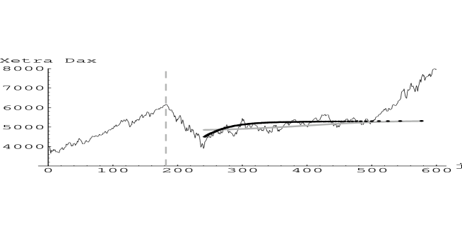
Figure 2. Long-lived asymmetric index profile,Xetra Dax Index from 23 X 1997 up to 10 III 2000 (600 close quotes) the numerical generalized least-squares estimator $\omega^{i}_{j}v_{i}$ of an unknown constant mean $m=E\{V_{j}\}$ of the field $V_{j};~{}j\subset i=1,\ldots,182$ (black dots) based on $v_{i}=v_{1},\ldots,v_{182}$ is compared for the negative correlation function (18) with the parameter $t=182+1,\ldots,182+139$ at finite $j\geq n+1=182+1$ to the classic generalized least-squares estimator $\lim_{j\rightarrow\infty}\omega^{i}_{j}v_{i}$ of an unknown constant mean $m=E\{V_{j}\}$ of the field $V_{j}$ (grey line) with the same correlation function and based on the same sample. The classic estimator is the first approximation of the numerical estimator at final $j=577$ for final $t=182+139$. The dashed vertical line represents $j=n=182$.

given at finite $j\geq n+1=182+1$ by numerical approximation to root of the equation (20). This (co-ordinate dependent) generalized least-squares estimator $\omega^{i}_{j}v_{i}$ was compared to the (co-ordinate independent) classic generalized least-squares estimator $\lim_{j\rightarrow\infty}\omega^{i}_{j}v_{i}$ of an unknown constant mean of the field (17)

$$\lim_{j\rightarrow\infty}w^{\prime}{\bf v}=\frac{F^{\prime}\Lambda^{-1}{\bf v}}{F^{\prime}\Lambda^{-1}F}$$

based on the same observation an initial amplification $v_{i}=v_{1},\ldots,v_{182}$ of long-lived asymmetric index profile recorded by $600$ close quotes of Xetra Dax Index shown in Fig. 2 then

$${\bf v}=\underbrace{\left[\begin{array}[]{c}v_{1}\\ \vdots\\ v_{182}\\ \end{array}\right]}_{n\times 1}$$

with the same correlation function (18).

Since the classic best linear unbiased generalized statistics for finite $n$ and $j\rightarrow\infty$ of an unknown constant mean $m=E\{V_{j}\}$ of the field $V_{j}$ with the constraint

$$\lim_{j\rightarrow\infty}E\{[V_{j}-\omega^{i}_{j}V_{i}]^{2}\}=\sigma^{2}=E\{[V_{j}-m]^{2}\}\ ,$$

is an asymptotic disjunction for $j\rightarrow\infty$ of the numerical best linear unbiased generalized statistics for finite $n$ at finite $j$ of an unknown constant mean $m=E\{V_{j}\}$ of the field $V_{j}$ with the constraint

$$E\{[V_{j}-\omega^{i}_{j}V_{i}]^{2}\}=\sigma^{2}=E\{[V_{j}-m]^{2}\}\ ,$$

then the correct classic generalized least-squares estimator $\lim_{j\rightarrow\infty}\omega^{i}_{j}v_{i}$ of an unknown constant mean $m$ of the field is an asymptotic disjunction for $j\rightarrow\infty$ of the numerical generalized least-squares estimator $\omega^{i}_{j}v_{i}$ of an unknowm constant mean $m$ of the field (see Fig. 2).

4. Summary

It was shown that the (estimation) statistics of the field $V_{j};j~{}\subset i=1,\ldots,n$ with an unknown constant mean $m$ and variance $\sigma^{2}$

$$\hat{V}_{j}=\sum_{i=1}^{n}\omega^{i}_{j}V_{i}=\omega^{i}_{j}V_{i}$$

that assumes – the unbiasedness constraint (2)

$$E\{V_{j}\}-E\{\omega^{i}_{j}V_{i}\}=0$$

that assumes – the minimization constraint (3)

$$\frac{\partial D^{2}\{V_{j}-\omega^{i}_{j}V_{j}\}}{\partial\omega^{i}_{j}}=0$$

given by the kriging system of equations (6)

$$\begin{array}[]{cccccl}{\underbrace{\left[\begin{array}[]{cccc}\rho_{\it 11}&\ldots&\rho_{\it 1n}&1\\ \vdots&\ddots&\vdots&\vdots\\ \rho_{\it n1}&\ldots&\rho_{\it nn}&1\\ 1&\ldots&1&0\\ \end{array}\right]}_{(n+1)\times(n+1)}}&\cdot&\underbrace{\left[\begin{array}[]{c}\omega_{j}^{\it 1}\\ \vdots\\ \omega_{j}^{\it n}\\ \mu^{\it 1}_{j}\\ \end{array}\right]}_{(n+1)\times 1}&=&\underbrace{\left[\begin{array}[]{c}\rho_{\it 1j}\\ \vdots\\ \rho_{\it nj}\\ 1\\ \end{array}\right]}_{(n+1)\times 1}\end{array}$$

is the best linear unbiased generalized (estimation) statistics of random field $V_{j}$ with minimized variance of the statistics

(21) $$E\{[\omega^{i}_{j}V_{i}-m]^{2}\}=\mp\sigma^{2}\left(\omega^{i}_{j}\rho_{ij}-\mu^{\it 1}_{j}\right)$$

and (minimized)

(22) $$E\{[V_{j}-\omega^{i}_{j}V_{i}]^{2}\}=\sigma^{2}\left(1\pm\left(\omega^{i}_{j}\rho_{ij}+\mu^{\it 1}_{j}\right)\right)$$

with the asymptotic property (Appendix B)

$$\lim_{n\rightarrow\infty}\lim_{j\rightarrow\infty}E\{[\omega^{i}_{j}V_{i}-m]^{2}\}=0$$

and

$$\lim_{n\rightarrow\infty}\lim_{j\rightarrow\infty}E\{[V_{j}-\omega^{i}_{j}V_{i}]^{2}\}=\sigma^{2}$$

constrained once again from (22) on computer – the third constraint of spatial statistics

$$E\{[V_{j}-\omega^{i}_{j}V_{i}]^{2}\}=\sigma^{2}=E\{[V_{j}-m]^{2}\}$$

is the numerical best linear unbiased generalized statistics for finite $n$ at finite $j$ of an unknown constant mean $m=E\{V_{j}\}$ of the field $V_{j}$ with the numerical generalized least-squares estimator $\omega^{i}_{j}v_{i}$ of an unknown constant mean of the field and its asymptotic disjunction for $j\rightarrow\infty$ the classic generalized least-squares estimator $\lim_{j\rightarrow\infty}\omega^{i}_{j}v_{i}$ of an unknown constant mean of the field.

Appendix A The sign of the terms

If for correlation matrix $\rho_{il};~{}i,l=1,\ldots,n$ that consists of unit diagonal elements (see (18)) and non-positive off-diagonal elements holds

$$\omega^{i}_{j}\rho_{il}\omega^{l}_{j}<0$$

like at $j\geq n+1$ for vector $\rho_{ij};~{}i=1,\ldots,n$ that consists of non-positive correlations holds

$$\omega^{i}_{j}\rho_{ij}<0$$

then (1)

$$D^{2}\{R_{j}\}=\sigma^{2}+2\sigma^{2}\omega^{i}_{j}\rho_{ij}-\sigma^{2}\omega^{i}_{j}\rho_{il}\omega^{l}_{j}$$

for non-negative correlation function

$$D^{2}\{R_{j}\}=\sigma^{2}-2\sigma^{2}\omega^{i}_{j}\rho_{ij}+\sigma^{2}\omega^{i}_{j}\rho_{il}\omega^{l}_{j}$$

for white noise

$$D^{2}\{R_{j}\}=\sigma^{2}+\sigma^{2}\omega^{i}_{j}\rho_{il}\omega^{l}_{j}\ ,$$

where $\rho_{il}$ is the identity matrix.

Appendix B The asymptotic property of the best linear unbiased generalized statistics of random field

From the minimization constraint (3)

$$\rho_{is}\omega^{s}_{j}+f_{\it i1}\mu^{\it 1}_{j}=\rho_{ij}$$

we get

$$\delta^{l}_{s}\omega^{s}_{j}=\omega^{l}_{j}=-\rho^{li}f_{\it i1}\mu^{\it 1}_{j}+\rho^{li}\rho_{ij}\ ,$$

where

$$\rho^{li}\rho_{is}=\delta^{l}_{s}\ ,$$

substituted into (2)

$$f_{\it 1l}\omega^{l}_{j}=1$$

gives

$$\mu^{\it 1}_{j}=(f_{\it 1l}\rho^{li}f_{\it i1})^{-1}(f_{\it 1l}\rho^{li}\rho_{ij}-1)$$

for $j\rightarrow\infty$ (9)

$$\rho_{ij}=\xi f_{\it i1}$$

then the Lagrange parameter simplifies to

$$\lim_{j\rightarrow\infty}\mu^{\it 1}_{j}=\xi-(f_{\it 1l}\rho^{li}f_{\it i1})^{-1}$$

from the unbiasedness condition (2) it also holds

$$\lim_{j\rightarrow\infty}\omega^{i}_{j}\rho_{ij}=\xi\omega^{i}_{j}f_{\it i1}=\xi$$

then the minimized variance of the estimation statistics (4)

$$E\{[\omega^{i}_{j}V_{i}-m]^{2}\}=\mp\sigma^{2}(\omega^{i}_{j}\rho_{ij}-\mu^{\it 1}_{j})$$

simplifies to

$$\lim_{j\rightarrow\infty}E\{[\omega^{i}_{j}V_{i}-m]^{2}\}=\mp\sigma^{2}\left(\xi-\xi+(f_{\it 1l}\rho^{li}f_{\it i1})^{-1}\right)$$

and (5)

$$E\{[V_{j}-\omega^{i}_{j}V_{i}]^{2}\}=\sigma^{2}(1\pm(\omega^{i}_{j}\rho_{ij}+\mu^{\it 1}_{j}))$$

simplifies to

$$\lim_{j\rightarrow\infty}E\{[V_{j}-\omega^{i}_{j}V_{i}]^{2}\}=\sigma^{2}(1\pm(\xi+\xi-(f_{\it 1l}\rho^{li}f_{\it i1})^{-1}))$$

since

$$\lim_{n\rightarrow\infty}\left(f_{\it 1l}\rho^{li}f_{\it i1}\right)^{-1}=0$$

and

$$\xi\rightarrow 0$$

we get the asymptotic property of the best linear unbiased generalized statistics of random field

$$\lim_{n\rightarrow\infty}\lim_{j\rightarrow\infty}E\{[\omega^{i}_{j}V_{i}-m]^{2}\}=0$$

and

$$\lim_{n\rightarrow\infty}\lim_{j\rightarrow\infty}E\{[V_{j}-\omega^{i}_{j}V_{i}]^{2}\}=\sigma^{2}\ .$$

References

• [1] E. H. Isaaks and R. M. Srivastava, An Introduction to Applied Geostatistics, New York: Oxford Univ. Press (1989).