Analysis of the consistency of parity-odd
nonbirefringent modified Maxwell theory

Abstract

There exist two deformations of standard electrodynamics that describe Lorentz symmetry violation in the photon sector: CPT-odd Maxwell–Chern–Simons theory and CPT-even modified Maxwell theory. In this article, we focus on the parity-odd nonbirefringent sector of modified Maxwell theory. It is coupled to a standard Dirac theory of massive spin-1/2 fermions resulting in a modified quantum electrodynamics (QED). This theory is discussed with respect to properties such as microcausality and unitarity, where it turns out that these hold.

Furthermore, a priori, the limit of the theory for vanishing Lorentz-violating parameters seems to be discontinuous. The modified photon polarization vectors are interweaved with preferred spacetime directions defined by the theory and one vector even has a longitudinal part. That structure remains in the limit mentioned. Since it is not clear, whether or not this behavior is a gauge artifact, the cross section for a physical process — modified Compton scattering — is calculated numerically. Despite the numerical instabilities occurring for scattering of unpolarized electrons off polarized photons in the second physical polarization state, it is shown that for Lorentz-violating parameters much smaller than one, the modified cross sections approach the standard QED results. Analytical investigations strengthen the numerical computations.

Hence, the theory proves to be consistent, at least with regard to the investigations performed. This leads to the interesting outcome of the modification being a well-defined parity-odd extension of QED.

I Introduction

Modern quantum field theories are based on fundamental symmetries. This holds for quantum electrodynamics (QED) as well as for the standard model of elementary particle physics. Whenever physicists talk about symmetries they usually think of gauge invariance or the discrete symmetries charge conjugation C, parity P, and time reversal T. However, there is one symmetry that often takes a back seat: Lorentz invariance. This is not surprising, since until now there had been no convincing experimental evidence for a violation of Lorentz invariance.

However, a violation of other symmetries is part of the everyday life of any high-energy physicist. For example, violations of P and CP were measured long ago Wu:1957 ; Christenson:1964fg and a broken electroweak gauge symmetry with massive $\mathrm{W^{\pm}}$, and $\mathrm{Z^{0}}$ bosons is an experimental fact. Why then should Lorentz symmetry and its violation not be of interest?

There exist good theoretical arguments for Lorentz invariance being a symmetry that is restored at low energies ChadhaNielsen1983 . At the Planck length the topology of spacetime may be dynamical, which could lead to it having a foamy structure. The existence of such a spacetime foam Wheeler:1957mu ; Hawking:1979zw may define a preferred reference frame — as is the case for water in a glass — and thus violate Lorentz invariance. Since a fundamental quantum theory of spacetime is still not known, we have to rely on well-established theories such as the standard model or special relativity for a description of Lorentz violation. By introducing new parameters that deform these theories it is possible to parameterize Lorentz violation on the basis of standard physics. One approach is to modify dispersion relations of particles. However, such a procedure is very ad hoc and it is not evident where the modification comes from. Therefore, a more elementary possibility is to parameterize modifications on the level of Lagrange densities. A collection of all Lorentz-violating deformations of the standard model that are gauge invariant is known as the Lorentz-violating extension of the standard model ColladayKostelecky1998 . The minimal version of this extension relies on power-counting renormalizable terms, whereas the nonminimal version also includes operators of mass dimension $d>4$ (see e.g. the analyses performed in Kostelecky:2009zp ; Kostelecky:2011gq ; Cambiaso:2012vb ).

The theoretical consistency of the standard model itself has been verified by investigations based on Lorentz-invariant quantum field theory that were performed over decades (see, for example, Ref. JordanPauli1928 ). However, it is not entirely clear if a Lorentz-violating theory is consistent. Some results on certain sectors of the standard model extension already exist KosteleckyLehnert2000 ; AdamKlinkhamer2001 ; Liberati:2001sd ; Mavromatos:2009xg ; Casana-etal2009 ; Casana-etal2010 ; Klinkhamer:2010zs ; Klinkhamer:2011ez , but there still remains a lot what we can learn about Lorentz-violating quantum field theories. Because of this it is very important to check Lorentz-violating deformations with respect to fundamental properties such as microcausality and unitarity. Furthermore, it is of significance whether the modified theory approaches the standard theory for arbitrarily small deformations. The purpose of this paper is to investigate these questions.

Especially in the case where Lorentz violation resides in the photon sector, it can lead to a variety of new effects, for example a birefringent vacuum ColladayKostelecky1998 , new particle decays Beall:1970rw ; Coleman:1997xq , and “aetherlike” deviations from special relativity, which are modulated with the rotation of the Earth around the Sun (e.g. Refs. Phillips:2000dr ; Bear:2000cd ). From an experimental point of view, photons produce clean signals making the photon sector very important, in bounding Lorentz-violating parameters.

There exist two gauge-invariant and power-counting renormalizable deformations of the photon sector: Maxwell–Chern–Simons theory (MCS-theory) Carroll-etal1990 and modified Maxwell theory ColladayKostelecky1998 ; KosteleckyMewes2002 . Each Lagrangian contains additional terms besides the Maxwell term of standard electrodynamics. The consistency of the isotropic and one anisotropic sector of modified Maxwell theory was already shown in Klinkhamer:2010zs . In this article a special sector, that violates parity and is supposed to show no birefringence, will be investigated.

The paper is organized as follows. In Sec. 2 modified Maxwell theory is presented and restricted to the parity-odd nonbirefringent case. Additionally, it is coupled to a standard Dirac theory of massive spin-1/2 fermions, which leads to a theory of modified QED. In Secs. 3 and 4, we review the nonstandard photon dispersion relations and the gauge propagator, which are determined from the field equations Casana-etal2009 ; Casana-etal2010 . That completes the current status of research concerning this special sector of modified Maxwell theory. The successive parts of the article deal with the main issue, beginning with the deformed polarization vectors, which can also be obtained from the field equations. After setting up the building blocks we are ready to discuss unitarity in Sec. 6 and microcausality in Sec. 7. The subsequent two sections are devoted to the polarization vectors themselves. Since their form is rather uncommon — even when considering Lorentz-violating theories — we make comparisons with MCS-theory and other sectors of modified Maxwell theory. It will become evident that the polarization vectors have a property that distinguishes them from the polarization vectors of standard electrodynamics, even in the limit of vanishing Lorentz violation. To test, whether or not some residue of the deformation remains in this limit, in Sec. 9 we compute the cross section of the simplest tree-level process involving external modified photons that is also allowed by standard QED: Compton scattering. We conclude in the last section. Readers may skip Secs. 4 – 8 on first reading.

II Modified Maxwell theory

II.1 Action and nonbirefringent Ansatz

In this article, we focus on modified Maxwell theory ChadhaNielsen1983 ; ColladayKostelecky1998 ; KosteleckyMewes2002 . This particular Lorentz-violating theory is characterized by the action

$$S_{\mathrm{modMax}} = \int_{\mathbb{R}^{4}}\mathrm{d}^{4}x\,\mathcal{L}_{\text{modMax}}(x)\,,$$ (2.1a)

$$\mathcal{L}_{\text{modMax}}(x) = -\frac{1}{4}\,\eta^{\mu\rho}\,\eta^{\nu\sigma}\,F_{\mu\nu}(x)F_{\rho\sigma}(x)-\frac{1}{4}\,\kappa^{\mu\nu\varrho\sigma}\,F_{\mu\nu}(x)F_{\varrho\sigma}(x)\,,$$ (2.1b)

which involves the field strength tensor $F_{\mu\nu}(x)\equiv\partial_{\mu}A_{\nu}(x)-\partial_{\nu}A_{\mu}(x)$ of the $U(1)$ gauge field $A_{\mu}(x)$. The fields are defined on Minkowski spacetime with global Cartesian coordinates $(x^{\mu})$ $=$ $(x^{0},\boldsymbol{x})$ $=$ $(c\,t,x^{1},x^{2},x^{3})$ and metric $g_{\mu\nu}(x)$ $=$ $\eta_{\mu\nu}$ $\equiv$ $\text{diag}\,(1,\,-1,\,-1,\,-1)\,$. The first term in Eq. (2.1b) represents the standard Maxwell term and the second corresponds to a modification of the standard theory of photons. The fixed background field $\kappa^{\mu\nu\varrho\sigma}$ selects preferred directions in spacetime and, therefore, breaks Lorentz invariance.

The second term in Eq. (2.1b) is expected to have the same symmetries as the first. These correspond to the symmetries of the Riemann curvature tensor, which reduces the number of independent parameters to 20. Furthermore, a vanishing double trace, $\kappa^{\mu\nu}_{\phantom{\mu\nu}\mu\nu}=0$, is imposed. A nonvanishing $\kappa^{\mu\nu}_{\phantom{\mu\nu}\mu\nu}$ can be absorbed by a field redefinition ColladayKostelecky1998 and does not contribute to physical observables. This additional condition leads to a remaining number of 19 independent parameters.

Modified Maxwell theory has two distinct parameter sectors that can be distinguished from each other by the property of birefringence. The first consists of 10 parameters and leads to birefringent photon modes at leading-order Lorentz violation. The second is made up of 9 parameters and shows no birefringence, at least to first order with respect to the parameters. Since the 10 birefringent parameters are bounded by experiment at the $10^{-32}$ level Kostelecky:2001mb , we will restrict our considerations to the nonbirefringent sector, which can be parameterized by the following Ansatz BaileyKostelecky2004 :

$$\kappa^{\mu\nu\varrho\sigma}=\frac{1}{2}\,\Big{(}\eta^{\mu\varrho}\,\widetilde{\kappa}^{\nu\sigma}-\eta^{\mu\sigma}\,\widetilde{\kappa}^{\nu\varrho}-\eta^{\nu\varrho}\,\widetilde{\kappa}^{\mu\sigma}+\eta^{\nu\sigma}\,\widetilde{\kappa}^{\mu\varrho}\Big{)}\,,$$ (2.2)

with a constant symmetric and traceless $4\times 4$ matrix $\widetilde{\kappa}^{\mu\nu}$. Here and in the following, natural units are used with $\hbar=c=1$, where $c$ corresponds to the maximal attainable velocity of the standard Dirac particles, whose action will be defined in Sec. II.3.

There exists a premetric formulation of classical electrodynamics, that is solely based on the concept of a manifold and does not need a metric. In this context a tensor density $F$ (electromagnetic field strength) and pseudotensor densities $\mathcal{H}$, $\mathcal{J}$ (electromagnetic excitation and electric current) are introduced. Since the resulting field equations for these quantities are underdetermined, an additional relation between $F$ and $\mathcal{H}$ has to be imposed, which is governed by the so-called constitutive four-tensor $\chi$. Modified Maxwell theory emerges as one special case of this description, namely as the principal part of the constitutive tensor previously mentioned Hehl:2003 ; Itin:2009aa . In Eq. (D.1.80) of the book Hehl:2003 the nonbirefringent Ansatz of Eq. (2.2) can be found, as well. Section D.1.6 gives a motivation for it as the simplest — but not the most general — decomposition of the principal part of $\chi$.

Furthermore, note that a special sector of CPT-even modified Maxwell theory arises as a contribution of the one-loop effective action of a CPT-odd deformation involving a spinor field and the photon field Gomes:2009ch .

II.2 Restriction to the parity-odd anisotropic case

The anisotropic case considered concerns the parity-odd sector of modified Maxwell theory (2.1) with the Ansatz from Eq. (2.2). This case is characterized by one purely timelike normalized four-vector $\xi^{\mu}$ and one purely spacelike four-vector $\zeta^{\mu}$ containing three real parameters $\widetilde{\kappa}^{01}$, $\widetilde{\kappa}^{02}$, and $\widetilde{\kappa}^{03}$ :

$$\widetilde{\kappa}^{\mu\nu} = \frac{1}{2}\,(\xi^{\mu}\zeta^{\nu}+\zeta^{\mu}\xi^{\nu})-\frac{1}{4}\,\xi^{\lambda}\zeta_{\lambda}\,\eta^{\mu\nu}\,,$$ (2.3a)

$$(\xi^{\mu}) = (1,\,0,\,0,\,0)\,,\quad(\zeta^{\mu})\equiv(0,\,2\,\boldsymbol{\zeta})=(0,\,2\,\widetilde{\kappa}^{01},\,2\,\widetilde{\kappa}^{02},\,2\,\widetilde{\kappa}^{03})\,,$$ (2.3b)

$$(\widetilde{\kappa}^{\mu\nu}) = \begin{pmatrix}0&\widetilde{\kappa}^{01}&\widetilde{\kappa}^{02}&\widetilde{\kappa}^{03}\\ \widetilde{\kappa}^{01}&0&0&0\\ \widetilde{\kappa}^{02}&0&0&0\\ \widetilde{\kappa}^{03}&0&0&0\\ \end{pmatrix}\,,$$ (2.3c)

where (2.3a) is the most general Ansatz for a symmetric and traceless tensor constructed from two four-vectors. The second term on the right-hand side of (2.3a) vanishes for the special choice (2.3b).

With the replacement rules given in KlinkhamerRisse2008b , we can express our parameters in terms of the Standard Model Extension (SME) parameters KosteleckyMewes2002 ; BaileyKostelecky2004 :

$$\widetilde{\kappa}^{01} = -(\widetilde{\kappa}_{\mathrm{o}+})^{(23)}\,,$$ (2.4a)

$$\widetilde{\kappa}^{02} = -(\widetilde{\kappa}_{\mathrm{o}+})^{(31)}\,,$$ (2.4b)

$$\widetilde{\kappa}^{03} = -(\widetilde{\kappa}_{\mathrm{o}+})^{(12)}\,.$$ (2.4c)

Hence, the case considered here includes only parity-violating coefficients.

This parity-odd case may be of relevance, since it might reflect the parity-odd low-energy effective photon sector of a quantum theory of spacetime. Besides five parameters of the birefringent sector of modified Maxwell theory, whose coefficients are already strongly bounded, there is only one alternative parity-odd Lorentz-violating theory for the photon sector, which is gauge-invariant and power-counting renormalizable: MCS theory Carroll-etal1990 . However, the MCS parameters are bounded to lie below $10^{-42}\,\mathrm{GeV}$ by CMB polarization measurements Kostelecky:2008ts .

Since the bounds are not as strong for the parity-odd case of nonbirefringent modified Maxwell theory defined by Eq. (2.3), a physical understanding of this case is of importance.

II.3 Coupling to matter: Parity-odd modified QED

Modified photons are coupled to matter by the minimal coupling procedure to standard (Lorentz-invariant) spin-$\textstyle{\frac{1}{2}}$ Dirac particles with electric charge $e$ and mass $M$. This results in a parity-odd deformation of QED Heitler1954 ; JauchRohrlich1976 ; Veltman1994 , which is given by the action

$$S_{\text{modQED}}^{\text{parity-odd}}\big{[}\widetilde{\kappa}^{0m},e,M\big{]}=S_{\text{modMax}}^{\text{parity-odd}}\big{[}\widetilde{\kappa}^{0m}\big{]}+S^{\text{}}_{\text{Dirac}}\big{[}e,M\big{]}\,,$$ (2.5)

for $m=1$, 2, 3 and with the modified-Maxwell term (2.1)–(2.3) for the gauge field $A_{\mu}(x)$ and the standard Dirac term for the spinor field $\psi(x)$,

$$S^{\text{ }}_{\text{Dirac}}\big{[}e,M\big{]}=\int_{\mathbb{R}^{4}}\mathrm{d}^{4}x\;\overline{\psi}(x)\Big{[}\gamma^{\mu}\big{(}\mathrm{i}\,\partial_{\mu}-eA_{\mu}(x)\big{)}-M\Big{]}\psi(x)\,.$$ (2.6)

Equation (2.6) is to be understood with standard Dirac matrices $\gamma^{\mu}$ corresponding to the Minkowski metric $\eta^{\mu\nu}$.

III Dispersion relations

The field equations ColladayKostelecky1998 ; KosteleckyMewes2002 ; BaileyKostelecky2004 of modified Maxwell theory in momentum space,

$$M^{\mu\nu}A_{\nu}=0\,,\quad M^{\mu\nu}\equiv k^{\lambda}k_{\lambda}\,\eta^{\mu\nu}-k^{\mu}k^{\nu}-2\,\kappa^{\mu\rho\sigma\nu}\,k_{\rho}k_{\sigma}\,,$$ (3.1)

lead to the following dispersion relations Casana-etal2009 for the two physical degrees of freedom of electromagnetic waves (labeled $\lambda=1,2$):

$$\omega_{1}(\mathbf{k}) = \widetilde{\kappa}^{01}\,k_{1}+\widetilde{\kappa}^{02}\,k_{2}+\widetilde{\kappa}^{03}\,k_{3}+\sqrt{|\mathbf{k}|^{2}+(\widetilde{\kappa}^{01}\,k_{1}+\widetilde{\kappa}^{02}\,k_{2}+\widetilde{\kappa}^{03}\,k_{3})^{2}}\,,$$ (3.2a)

$$\omega_{2}(\mathbf{k}) = \widetilde{\kappa}^{01}k_{1}\,+\widetilde{\kappa}^{02}k_{2}\,+\widetilde{\kappa}^{03}k_{3}\,+\sqrt{1+(\widetilde{\kappa}^{01})^{2}+(\widetilde{\kappa}^{02})^{2}+(\widetilde{\kappa}^{03})^{2}}\;|\mathbf{k}|\,,$$ (3.2b)

for wave vector $\mathbf{k}=(k_{1},\,k_{2},\,k_{3})$ and with the terms linear in the components $k_{m}$ explicitly showing the parity violation. To first order in $\widetilde{\kappa}^{0m}$, the dispersion relations are equal for both modes, but they differ at higher order. With the modified Coulomb and Ampère law it can be shown that the dispersion relations (3.2) indeed belong to physical photon modes. The procedure given in ColladayKostelecky1998 eliminates dispersion relations of unphysical, i.e. scalar and longitudinal, modes from the field equations. The two are given by

$$\omega_{0}(\mathbf{k})=\omega_{3}(\mathbf{k})=|\mathbf{k}|\,,$$ (3.3)

where the index “0” refers to the scalar and the index “3” to the longitudinal degree of freedom of the photon field.

The dispersion relations (3.2) can be cast in a more compact form by defining components of the wave-vector $\mathbf{k}$ which are parallel or orthogonal to the background “three-vector” $\boldsymbol{\zeta}$:

$$k_{\|}=\mathbf{k}\cdot\widehat{\boldsymbol{\zeta}}\,,\quad k_{\bot}=|\mathbf{k}-(\mathbf{k}\cdot\widehat{\boldsymbol{\zeta}})\,\widehat{\boldsymbol{\zeta}}|\,,\quad\widehat{\boldsymbol{\zeta}}\equiv\frac{1}{\sqrt{(\widetilde{\kappa}^{01})^{2}+(\widetilde{\kappa}^{02})^{2}+(\widetilde{\kappa}^{03})^{2}}}\begin{pmatrix}\widetilde{\kappa}^{01}\\ \widetilde{\kappa}^{02}\\ \widetilde{\kappa}^{03}\\ \end{pmatrix}\,,$$ (3.4)

where $k_{\parallel}\in(-\infty,\infty)$ and $k_{\bot}\in[0,\infty)$. By doing so, it is possible to write the dispersion relations (3.2) as follows:

$$\omega_{1}(k_{\bot},k_{\|})=\mathcal{E}\,k_{\|}+\sqrt{k_{\bot}^{2}+(1+\mathcal{E}^{2})\,k_{\|}^{2}}\,,$$ (3.5a)

$$\omega_{2}(k_{\bot},k_{\|})=\mathcal{E}\,k_{\parallel}+\sqrt{1+\mathcal{E}^{2}}\,|\mathbf{k}|\,,$$ (3.5b)

where the three Lorentz-violating parameters $$\widetilde{\kappa}^{01} \widetilde{\kappa}^{02} \widetilde{\kappa}^{03} \mathcal{E}$$, , and are contained in the single parameter that is defined as

$$\mathcal{E}\equiv|\boldsymbol{\zeta}|\equiv\sqrt{(\widetilde{\kappa}^{01})^{2}+(\widetilde{\kappa}^{02})^{2}+(\widetilde{\kappa}^{03})^{2}}\,.$$ (3.5c)

It is obvious that $\mathcal{E}\in[0,\infty)$, whereas each single parameter $\widetilde{\kappa}^{01}$, $\widetilde{\kappa}^{02}$, and $\widetilde{\kappa}^{03}$ can be either positive or negative. From the first definition of Eq. (3.4) we see that negative parameters $\widetilde{\kappa}^{01}$, $\widetilde{\kappa}^{02}$, $\widetilde{\kappa}^{03}$ are mimicked by a negative $k_{\parallel}$.

The phase and group velocity Brillouin1960 of the above two modes can be cast in the following form for small enough $\mathcal{E}$:

$$v_{\mathrm{ph},\,1}\equiv\frac{\omega_{1}}{|\mathbf{k}|}=1+\mathcal{E}\cos\theta+\frac{\mathcal{E}^{2}}{2}\cos^{2}\theta+\mathsf{O}(\mathcal{E}^{3})\,,$$ (3.6a)

$$v_{\mathrm{ph},\,2}\equiv\frac{\omega_{2}}{|\mathbf{k}|}=1+\mathcal{E}\cos\theta+\frac{\mathcal{E}^{2}}{2}+\mathsf{O}(\mathcal{E}^{3})\,,$$ (3.6b)

$$v_{\mathrm{gr},\,1}\equiv\left|\frac{\partial\omega_{1}}{\partial\mathbf{k}}\right|=1+\mathcal{E}\cos\theta+\frac{\mathcal{E}^{2}}{2}+\mathsf{O}(\mathcal{E}^{3})\,,$$ (3.7a)

$$v_{\mathrm{gr},\,2}\equiv\left|\frac{\partial\omega_{2}}{\partial\mathbf{k}}\right|=1+\mathcal{E}\cos\theta+\left(1+\sin^{2}\theta\right)\frac{\mathcal{E}^{2}}{2}+\mathsf{O}(\mathcal{E}^{3})\,,$$ (3.7b)

where $\theta$ is the angle between the three-momentum $\mathbf{k}$ and the unit vector $\widehat{\boldsymbol{\zeta}}$: $\cos\theta=\mathbf{k}\cdot\widehat{\boldsymbol{\zeta}}/|\mathbf{k}|$.

To leading order in $\mathcal{E}$, the velocities above are equal:

$$v_{\mathrm{ph},\,1}=v_{\mathrm{ph},\,2}=v_{\mathrm{gr},\,1}=v_{\mathrm{gr},\,2}\,.$$ (3.8)

Furthermore, Eqs. (3.6), (3.7) show that both phase and group velocity can be larger than 1. However, what matters physically is the velocity of signal propagation, which corresponds to the front velocity Brillouin1960 :

$$v_{\mathrm{fr}}\equiv\lim_{k\mapsto\infty}v_{\mathrm{ph}}\,.$$ (3.9)

Equation (3.9) can be interpreted as the velocity of the highest-frequency forerunners of a signal. As can be seen from Eq. (3.6), $v_{\mathrm{ph}}$ and hence also $v_{\mathrm{fr}}$ do not depend on the magnitude of the wave vector, but only on its direction. For $\mathcal{E}\ll 1$, we obtain $v_{\mathrm{fr},\,1}\simeq v_{\mathrm{fr},\,2}\equiv v_{\mathrm{fr}}$, where

$$v_{\mathrm{fr}} < 1\;\;\text{for}\;\;\pi/2<\theta<3\pi/2\,,$$ (3.10a)

$$v_{\mathrm{fr}} \geq 1\;\;\text{for}\;\;0\leq\theta\leq\pi/2\;\vee\;3\pi/2\leq\theta<2\pi\,.$$ (3.10b)

Observe that, for small enough $\mathcal{E}$, having $v_{\mathrm{fr}}<1$ or $v_{\mathrm{fr}}\geq 1$ does not depend on the Lorentz-violating parameters but only on the direction in which the classical wave propagates. For completeness, we also give the phase velocities for propagation parallel and orthogonal to $\widehat{\boldsymbol{\zeta}}$:

$$v_{\mathrm{ph},\|,\,1}=\frac{\omega_{1}(k_{\bot},k_{\|})}{k_{\|}}\,\Bigg{|}_{k_{\bot}=0}=\mathcal{E}\,\mathrm{sgn}(k_{\parallel})+\sqrt{1+\mathcal{E}^{2}}=v_{\mathrm{ph},\|,\,2}\,,$$ (3.11a)

$$v_{\mathrm{ph},\bot,\,1}=\frac{\omega_{1}(k_{\bot},k_{\|})}{k_{\bot}}\,\Bigg{|}_{k_{\|}=0}=1\,,\quad v_{\mathrm{ph},\bot,\,2}=\frac{\omega_{2}(k_{\bot},k_{\|})}{k_{\bot}}\,\Bigg{|}_{k_{\|}=0}=\sqrt{1+\mathcal{E}^{2}}\,,$$ (3.11b)

with the sign function

$$\mathrm{sgn}(x)=\left\{\begin{array}[]{rcl}1&\text{for}&x>0\,,\\ 0&\text{for}&x=0\,,\\ -1&\text{for}&x<0\,.\\ \end{array}\right.$$ (3.12)

Note that the latter results are in agreement with the inequalities of Eq. (3.10). We conclude that the front velocity can be larger than 1 for the wave vector pointing in certain directions. That leads us to the issue of microcausality, which will be discussed in Sec. VII.

IV Propagator in the Feynman gauge

So far, we have investigated the dispersion relations of the classical theory. For a further analysis, especially concerning the quantum theory, the gauge propagator will be needed. The propagator is the Green’s function of the free field equations (3.1) in momentum space. In order to compute it the gauge has to be fixed. We decide to use the Feynman gauge Veltman1994 ; ItzyksonZuber1980 ; PeskinSchroeder1995 , which can be implemented by the gauge-fixing condition

$$\mathcal{L}_{\mathrm{gf}}(x)=-\frac{1}{2}\big{(}\partial_{\mu}\,A^{\mu}(x)\big{)}^{2}\,.$$ (4.1)

The following Ansatz for the propagator turns out to be useful:

$$\widehat{G}_{\nu\lambda}\,\big{|}^{\mathrm{Feynman}}=-\mathrm{i}\,\Big{\{} +\widehat{a}\,\eta_{\nu\lambda}+\widehat{b}\,k_{\nu}k_{\lambda}+\widehat{c}\,\xi_{\nu}\xi_{\lambda}+\widehat{d}\,(k_{\nu}\xi_{\lambda}+\xi_{\nu}k_{\lambda})$$

$$+\widehat{e}\,\zeta_{\nu}\zeta_{\lambda}+\widehat{f}\,(k_{\nu}\zeta_{\lambda}+\zeta_{\nu}k_{\lambda})+\widehat{g}\,(\xi_{\nu}\zeta_{\lambda}+\zeta_{\nu}\xi_{\lambda})\Big{\}}\,\widehat{K}_{1}\,.$$ (4.2)

The propagator coefficients $\widehat{a}=\widehat{a}(k^{0},\mathbf{k})$, $\ldots$, $\widehat{g}=\widehat{g}(k^{0},\mathbf{k})$ and the scalar propagator part $\widehat{K}_{1}=\widehat{K}_{1}(k^{0},\mathbf{k})$ follow from the system of equations $(\widehat{G}^{-1})^{\mu\nu}\widehat{G}_{\nu\lambda}=\mathrm{i}\,\delta^{\mu}_{\phantom{\mu}\lambda}$ with the differential operator

$$(G^{-1})^{\mu\nu}=\eta^{\mu\nu}\partial^{2}-2\,\kappa^{\mu\varrho\sigma\nu}\partial_{\varrho}\partial_{\sigma}\,,$$ (4.3)

in Feynman gauge transformed to momentum space. Scalar products $\xi^{\mu}\xi_{\mu}$, $\zeta^{\mu}\zeta_{\mu}$, and $\xi^{\mu}\zeta_{\mu}$ will be kept in the result, in order to gain some insight in the covariant structure of the functions. However, we remark that, for the case considered, $\xi^{2}\equiv\xi^{\mu}\xi_{\mu}=1$, $\zeta^{2}\equiv\zeta^{\mu}\zeta_{\mu}=-4\mathcal{E}^{2}$, and $\xi\cdot\zeta\equiv\xi^{\mu}\zeta_{\mu}=0$.

Specifically, the propagator coefficients and the scalar propagators $\widehat{K}_{1}$ and $\widehat{K}_{2}$, where $\widehat{K}_{2}$ appears in some of these coefficients, are given by

$$\widehat{K}_{1} = \frac{2}{2\,k\cdot\xi\,k\cdot\zeta+k^{2}\,\big{(}2-\xi\cdot\zeta\big{)}}\,,$$ (4.4a)

$$\widehat{K}_{2} \equiv \frac{4}{4\,k\cdot\xi\,k\cdot\zeta+\xi^{2}(k\cdot\zeta)^{2}+\zeta^{2}(k\cdot\xi)^{2}+k^{2}(4-\xi^{2}\zeta^{2})}\,,$$ (4.4b)

$$\widehat{a}=1\,,$$ (4.5a)

$$\widehat{b} =-\frac{1}{4\,k^{4}}\left\{\Upsilon\,\widehat{K}_{2}-2\,\chi\,\Big{(}2\,k\cdot\xi\,k\cdot\zeta+k^{2}(2-\xi\cdot\zeta)\Big{)}\right\}\,,$$ (4.5b)

$$\widehat{c}=\frac{1}{4}\big{[}k^{2}\zeta^{2}-(k\cdot\zeta)^{2}\big{]}\,\widehat{K}_{2}\,,$$ (4.5c)

$$\widehat{d}=\frac{k\cdot\xi\big{(}2\,(k\cdot\zeta)^{2}-k^{2}\zeta^{2}\big{)}+2\,k^{2}\,k\cdot\zeta}{4\,k^{2}}\,\widehat{K}_{2}\,,$$ (4.5d)

$$\widehat{e}=\frac{1}{4}\big{[}k^{2}\xi^{2}-(k\cdot\xi)^{2}\big{]}\,\widehat{K}_{2}\,,$$ (4.5e)

$$\widehat{f}=\frac{k\cdot\zeta\big{(}2\,(k\cdot\xi)^{2}-k^{2}\xi^{2}\big{)}+2\,k^{2}\,k\cdot\xi}{4\,k^{2}}\,\widehat{K}_{2}\,,$$ (4.5f)

$$\Upsilon \equiv -2\,k\cdot\xi\,k\cdot\zeta(2\,k^{2}-k\cdot\xi\,k\cdot\zeta)+(k\cdot\zeta)^{2}\big{(}(k\cdot\xi)^{2}-k^{2}\xi^{2}\big{)}$$ (4.5g)

$$\quad\,+(k\cdot\xi)^{2}\big{[}(k\cdot\zeta)^{2}-k^{2}\zeta^{2}\big{]}+k^{2}\big{[}12\,k\cdot\xi\,k\cdot\zeta+\xi^{2}(k\cdot\zeta)^{2}$$

$$\quad\,+\zeta^{2}(k\cdot\xi)^{2}+k^{2}(4-\xi^{2}\zeta^{2})\big{]}\,,$$

$$\widehat{g}=-\frac{1}{4}\big{[}2\,k^{2}+k\cdot\xi\,k\cdot\zeta\big{]}\,\widehat{K}_{2}\,,$$ (4.5h)

where definition (4.5g) enters (4.5b).

The poles of $\widehat{K}_{1}$ and $\widehat{K}_{2}$ can be identified with the dispersion relations obtained in Sec. III. From $\widehat{K}_{1}(\omega_{1},\mathbf{k})^{-1}=0$, that is

$$2\,k\cdot\xi\,k\cdot\zeta+k^{2}\,\big{(}2-\xi\cdot\zeta\big{)}\,\Big{|}_{k_{0}=\omega_{1}}=0\,,$$ (4.6)

the dispersion relation (3.2a) of the $\lambda=1$ mode is recovered. Similarly, the dispersion relation (3.2b) of the $\lambda=2$ mode follows from $\widehat{K}_{2}(\omega_{2},\mathbf{k})^{-1}=0$, that is

$$4\,k\cdot\xi\,k\cdot\zeta+\xi^{2}(k\cdot\zeta)^{2}+\zeta^{2}(k\cdot\xi)^{2}+k^{2}(4-\xi^{2}\zeta^{2})\,\Big{|}_{k_{0}=\omega_{2}}=0\,,$$ (4.7)

The third pole $k^{2}=0$ corresponds to the dispersion relation of scalar and longitudinal modes. This is clear from the fact that this pole appears only in the gauge-dependent coefficients $\widehat{b}$, $\widehat{d}$, and $\widehat{f}$. These are multiplied by at least one photon four-momentum and vanish by the Ward identity, if they couple to a conserved current PeskinSchroeder1995 . Since the Ward identity results from gauge invariance, it also holds for modified Maxwell theory, which is expected to be free of anomalies ColladayKostelecky1998 . Because of parity violation the physical poles are asymmetric with respect to the imaginary $k^{0}$-axis.

The above result (IV)– (4.5) equals the propagator given in Casana-etal2010 . Every propagator coefficient, which contains the scalar propagator $\widehat{K}_{2}$, is also multiplied by $\widehat{K}_{1}$. Hence, both modes appear together throughout the propagator and the question arises, whether they can be separated. It can be shown that the propagator can also be written in the following form:

$$\widehat{G}_{\mu\nu}(k)\big{|}^{\mathrm{Feynman}}=\sum_{n=1,2}\Xi_{\mu\nu}^{(n)}(k^{0},\mathbf{k})\,\Big{(}-\mathrm{i}\widehat{G}^{(n)}(k)\Big{)}\,,$$ (4.8)

where the tensor structure $\Xi_{\mu\nu}$ is the same for both parts, hence

$$\Xi_{\nu\lambda}^{(1)}=\Xi_{\nu\lambda}^{(2)}= +\widehat{a}\,\eta_{\nu\lambda}+\widehat{b}\,k_{\nu}k_{\lambda}+\widehat{c}\,\xi_{\nu}\xi_{\lambda}+\widehat{d}\,(k_{\nu}\xi_{\lambda}+\xi_{\nu}k_{\lambda})$$

$$+\widehat{e}\,\zeta_{\nu}\zeta_{\lambda}+\widehat{f}\,(k_{\nu}\zeta_{\lambda}+\zeta_{\nu}k_{\lambda})+\widehat{g}\,(\xi_{\nu}\zeta_{\lambda}+\zeta_{\nu}\xi_{\lambda})\,,$$ (4.9)

with the coefficients $\widehat{a}$, …, $\widehat{g}$ from Eq. (4.5). The scalar propagator functions are then given by:

$$\widehat{G}^{(1)}(k)=\frac{4\widehat{K}_{1}\widehat{K}_{2}^{-1}}{[(k\cdot\xi)^{2}-k^{2}]\zeta^{2}+(k\cdot\zeta)^{2}}\,,\quad\widehat{G}^{(2)}(k)=-\frac{4}{[(k\cdot\xi)^{2}-k^{2}]\zeta^{2}+(k\cdot\zeta)^{2}}\,.$$ (4.10)

The first part $\widehat{D}^{(1)}(k)$ contains both polarization modes encoded in $\widehat{K}_{1}$ and $\widehat{K}_{2}$, whereas the second part does not involve any mode. The denominator $[(k\cdot\xi)^{2}-k^{2}]\zeta^{2}+(k\cdot\zeta)^{2}$ that appears in both parts does not have a zero with respect to $k_{0}$, hence it contains no dispersion relation. So it does not seem that the polarization modes can be separated, such that each propagator part contains exactly one of the modes.

Finally, we can state that the structure of the propagator of parity-odd nonbirefringent modified Maxwell theory is rather unusual. In the next section we will compute the polarization vectors.

V Polarization vectors

In what follows, the physical (transverse) degrees of freedom will be labeled with (1) and (2), respectively. For a fixed nonzero “three-vector” $\boldsymbol{\zeta}$ and a generic wave vector $\mathbf{k}$, the polarization vector of the $\lambda=1$ mode reads

$$\big{(}\varepsilon^{(1)\,\mu}\big{)}=\frac{1}{\sqrt{N^{\prime}}}\;\big{(}0,\,\boldsymbol{\zeta}\times\mathbf{k}\big{)}\big{/}\big{|}\boldsymbol{\zeta}\times\mathbf{k}\big{|}\,,$$ (5.1)

where $N^{\prime}$ is a normalization factor to be given later. The polarization vector of the $\lambda=2$ mode is orthogonal to (5.1) and has a longitudinal component. It is given by

$$(\varepsilon^{(2)\,\mu})=\frac{1}{\sqrt{N^{\prime\prime}}}\frac{1}{\sqrt{|\boldsymbol{\varepsilon}^{(2)}|^{2}-(\varepsilon^{0})^{2}}}\left(\varepsilon^{0},\,\boldsymbol{\varepsilon}^{(2)}\right)\,,$$ (5.2)

with

$$\varepsilon^{0}=\frac{1}{4}\Big{(}k^{2}-(k\cdot\xi)^{2}\Big{)}\Big{(}(k\cdot\zeta)^{2}-\zeta^{2}\left[k^{2}-(k\cdot\xi)^{2}\right]\Big{)}\,,$$ (5.3a)

$$\boldsymbol{\varepsilon}^{(2)} =\left(2\,|\mathbf{k}|^{2}\,|\boldsymbol{\zeta}|^{2}-\frac{|\mathbf{k}\times(\mathbf{k}\times\boldsymbol{\zeta})|^{2}}{|\mathbf{k}|^{2}}+2\,\sqrt{1+|\boldsymbol{\zeta}|^{2}}\,|\mathbf{k}|\,(\mathbf{k}\cdot\boldsymbol{\zeta})\right)\mathbf{k}\times(\mathbf{k}\times\boldsymbol{\zeta})$$

$$\hskip 56.9055pt\,+\Big{(}\sqrt{1+|\boldsymbol{\zeta}|^{2}}\,|\mathbf{k}|+\mathbf{k}\cdot\boldsymbol{\zeta}\Big{)}\;\frac{|\mathbf{k}\times(\mathbf{k}\times\boldsymbol{\zeta})|^{2}}{|\mathbf{k}|^{2}}\;\mathbf{k}\,.$$ (5.3b)

The polarization vector $\varepsilon^{(1)}$ is a solution of the field equations (3.1), when $k^{0}$ is replaced by $\omega_{1}(\mathbf{k})$ from Eq. (3.2a). The polarization $\varepsilon^{(2)}$ is the corresponding solution for $k^{0}$ replaced by $\omega_{2}(\mathbf{k})$ from Eq. (3.2b). The normalization factors $N^{\prime}$ in (5.1) and $N^{\prime\prime}$ in (5.2) can be computed from the 00–component of the energy-momentum tensor. Note that the above polarization vectors have been calculated in the Lorentz gauge, $\partial_{\mu}\,A^{\mu}=0$.

For the Lorentz-violating decay processes considered, both the $\lambda=1$ and the $\lambda=2$ polarization modes contribute.

$$\overline{\varepsilon}^{(1)\,\mu}\varepsilon^{(1)\,\nu} =\frac{1}{N^{\prime}}\;\Bigl{\{}-\eta^{\mu\nu}+\widehat{\Gamma}_{1}k^{\mu}k^{\nu}+\widehat{\Delta}_{1}(k^{\mu}\xi^{\nu}+\xi^{\mu}k^{\nu})+\widehat{\Lambda}_{1}(k^{\mu}\zeta^{\nu}+\zeta^{\mu}k^{\nu})$$

$$\hskip 40.40285pt+\widehat{\Phi}_{1}\,\xi^{\mu}\xi^{\nu}+\widehat{\Psi}_{1}\,\zeta^{\mu}\zeta^{\nu}+\widehat{\Theta}_{1}\,\big{(}\xi^{\mu}\zeta^{\nu}+\zeta^{\nu}\xi^{\mu}\big{)}\,\Bigr{\}}\,\Big{|}_{k_{0}=\omega_{1}}\,,$$ (5.4)

with

$$\widehat{\Gamma}_{1}=\frac{\zeta^{2}}{Q}\,,\quad\widehat{\Delta}=\frac{\zeta^{2}\,\big{[}2k^{2}+k\cdot\xi\,k\cdot\zeta\big{]}}{Q(\zeta\cdot k)}\,,\quad\widehat{\Lambda}_{1}=-\frac{k\cdot\zeta}{Q}\,,$$ (5.5a)

$$\widehat{\Theta}_{1}=-\frac{2k^{2}+k\cdot\xi\,k\cdot\zeta}{Q}\,,\quad\widehat{\Psi}_{1}=\frac{k^{2}\,\xi^{2}-(k\cdot\xi)^{2}}{Q}\,,\quad\widehat{\Phi}_{1}=\frac{k^{2}\,\zeta^{2}-(k\cdot\zeta)^{2}}{Q}\,,$$ (5.5b)

$$N^{\prime}=\frac{1}{\omega_{1}}\sqrt{k_{\bot}^{2}+(1+\mathcal{E}^{2})\,k_{\|}^{2}}\,,\quad Q=\zeta^{2}\,\big{[}k^{2}-(k\cdot\xi)^{2}\big{]}-(k\cdot\zeta)^{2}\,,$$ (5.5c)

where $\omega_{1}=\omega_{1}(k_{\bot},k_{\|})$ is given by (3.5a). The denominator $Q$ vanishes only for $\widetilde{\kappa}^{01}=\widetilde{\kappa}^{02}=\widetilde{\kappa}^{03}=0$ or $k_{\bot}=0$. If the polarization tensor of the $\lambda=1$ mode is contracted with a gauge-invariant expression using the Ward identity, it can be replaced by $\Pi^{\mu\nu}|_{\lambda=1}$:

$$\overline{\varepsilon}^{(1)\,\mu}\varepsilon^{(1)\,\nu}\mapsto\Pi^{\mu\nu}|_{\lambda=1}\,,$$ (5.6a)

$$\Pi^{\mu\nu}|_{\lambda=1} \equiv\overline{\varepsilon}^{(1)\,\mu}\varepsilon^{(1)\,\nu}\;\big{|}^{\text{truncated}}$$

$$=\frac{1}{N^{\prime}}\;\Bigl{\{}-\eta^{\mu\nu}+\widehat{\Phi}_{1}\,\xi^{\mu}\xi^{\nu}+\widehat{\Psi}_{1}\,\zeta^{\mu}\zeta^{\nu}+\widehat{\Theta}_{1}\big{(}\xi^{\mu}\zeta^{\nu}+\zeta^{\nu}\xi^{\mu}\big{)}\Bigr{\}}\,\Big{|}_{k_{0}=\omega_{1}}\,.$$ (5.6b)

The polarization tensor of the $\lambda=2$ mode is lengthy and is best written up in terms of $k_{\|}$ and $k_{\bot}$ defined in (3.4).

$$\overline{\varepsilon}^{(2)\,\mu}\varepsilon^{(2)\,\nu} =\frac{1}{N^{\prime\prime}}\Big{\{}+\widehat{\Gamma}_{2}k^{\mu}k^{\nu}+\widehat{\Delta}_{2}(k^{\mu}\xi^{\nu}+\xi^{\mu}k^{\nu})+\widehat{\Lambda}_{2}(k^{\mu}\zeta^{\nu}+\zeta^{\mu}k^{\nu})$$

$$\hskip 42.10995pt+\widehat{\Phi}_{2}\xi^{\mu}\xi^{\nu}+\widehat{\Psi}_{2}\zeta^{\mu}\zeta^{\nu}+\widehat{\Theta}_{2}(\xi^{\mu}\zeta^{\nu}+\zeta^{\mu}\xi^{\nu})\Big{\}}\,\Big{|}_{k_{0}=\omega_{2}}\,,$$ (5.7)

with

$$\widehat{\Gamma}_{2}=\frac{\mathcal{E}^{4}}{\mathcal{N}}\Big{[}\mathcal{E}k_{\parallel}k_{\bot}^{2}+(2k_{\parallel}^{2}+k_{\bot}^{2})\omega_{2}\Big{]}^{2}\,,$$ (5.8a)

$$\widehat{\Delta}_{2}=\frac{\mathcal{E}^{4}}{\mathcal{N}}\Big{(}\mathcal{E}k_{\parallel}k_{\bot}^{2}+(2k_{\parallel}^{2}+k_{\bot}^{2})\omega_{2}\Big{)}\Big{\{}k_{\bot}^{2}|\mathbf{k}|^{2}-\mathcal{E}k_{\parallel}k_{\bot}^{2}\omega_{2}-\big{[}2k_{\parallel}^{2}+k_{\bot}^{2}\big{]}\omega_{2}^{2}\Big{\}}\,,$$ (5.8b)

$$\widehat{\Lambda}_{2}=-\frac{\mathcal{E}^{3}}{2\mathcal{N}}|\mathbf{k}|^{2}\Big{(}2k_{\parallel}\omega_{2}+\mathcal{E}k_{\bot}^{2}\Big{)}\Big{[}\mathcal{E}k_{\parallel}k_{\bot}^{2}+(2k_{\parallel}^{2}+k_{\bot}^{2})\omega_{2}\Big{]}\,,$$ (5.8c)

$$\widehat{\Phi}_{2}=\frac{\mathcal{E}^{4}}{\mathcal{N}}\Big{[}k_{\bot}^{2}(k_{\bot}^{2}-\omega_{2}^{2})-\mathcal{E}k_{\parallel}k_{\bot}^{2}\omega_{2}+k_{\parallel}^{2}(k_{\bot}^{2}-2\omega_{2}^{2})\Big{]}^{2}\,,$$ (5.8d)

$$\widehat{\Psi}_{2}=\frac{\mathcal{E}^{2}}{4\mathcal{N}}|\mathbf{k}|^{4}(\mathcal{E}k_{\bot}^{2}+2k_{\parallel}\omega_{2})^{2}\,,$$ (5.8e)

$$\widehat{\Theta}_{2}=\frac{\mathcal{E}^{3}}{2\mathcal{N}}|\mathbf{k}|^{2}(\mathcal{E}k_{\bot}^{2}+2k_{\parallel}\omega_{2})\Big{[}k_{\bot}^{2}(\omega_{2}^{2}-k_{\bot}^{2})+\mathcal{E}k_{\parallel}k_{\bot}^{2}\omega_{2}-k_{\parallel}^{2}(k_{\bot}^{2}-2\omega_{2}^{2})\Big{]}\,,$$ (5.8f)

$$N^{\prime\prime}=\frac{\mathcal{E}^{4}k_{\bot}^{2}}{2\omega_{2}^{2}\mathcal{N}}|\mathbf{k}|^{2}\Big{[} +(4k_{\parallel}^{2}+k_{\bot}^{2})\omega_{2}^{4}+4\mathcal{E}k_{\parallel}k_{\bot}^{2}\omega_{2}^{3}+\big{(}4k_{\parallel}^{4}+2k_{\bot}^{2}k_{\parallel}^{2}+(\mathcal{E}^{2}-2)k_{\bot}^{4}\big{)}\omega_{2}^{2}$$

$$+4\mathcal{E}k_{\parallel}k_{\bot}^{2}|\mathbf{k}|^{2}\omega_{2}+k_{\bot}^{2}|\mathbf{k}|^{2}(|\mathbf{k}|^{2}+\mathcal{E}^{2}k_{\bot}^{2})\Big{]}\,.$$ (5.8g)

where

$$\mathcal{N}=|\boldsymbol{\varepsilon}^{(2)}|^{2}-(\varepsilon^{0})^{2}\,,$$ (5.8h)

and $\omega_{2}=\omega_{2}(k_{\bot},k_{\|})$ is given by (3.5b). Again, if the tensor is contracted with a gauge-invariant expression, it can be replaced by $\Pi^{\mu\nu}|_{\lambda=2}$:

$$\overline{\varepsilon}^{(2)\,\mu}\varepsilon^{(2)\,\nu}\mapsto\Pi^{\mu\nu}|_{\lambda=2}\,,$$ (5.9a)

$$\Pi^{\mu\nu}|_{\lambda=2} \equiv\overline{\varepsilon}^{(2)\,\mu}\varepsilon^{(2)\,\nu}\;\big{|}^{\text{truncated}}$$

$$=\frac{1}{N^{\prime\prime}}\Big{\{}\widehat{\Phi}_{2}\xi^{\mu}\xi^{\nu}+\widehat{\Psi}_{2}\zeta^{\mu}\zeta^{\nu}+\widehat{\Theta}_{2}(\xi^{\mu}\zeta^{\nu}+\zeta^{\mu}\xi^{\nu})\Big{\}}\,\,\Big{|}_{k_{0}=\omega_{2}}\,.$$ (5.9b)

Finally it holds that

$$k_{\mu}\left(\overline{\varepsilon}^{(1)\,\mu}\varepsilon^{(1)\,\nu}\right)(k)=0\,,\quad\lim_{\mathcal{E}\mapsto 0}k_{\mu}\left(\overline{\varepsilon}^{(2)\,\mu}\varepsilon^{(2)\,\nu}\right)(k)=0\,,$$ (5.10)

where the second contraction only vanishes for $\mathcal{E}\mapsto 0$ due to the longitudinal part of $\varepsilon^{(2)\,\mu}$.

The polarization vector (5.2) is normalized to unit length by $\mathcal{N}$. This normalization factor cancels in $\Pi^{\mu\nu}|_{\lambda=2}$. Note that the metric tensor $\eta^{\mu\nu}$ does not appear on the right-hand side of (5.9), whereas it does on the right-hand side of Eq.  (5.6).

Furthermore, note that each truncated polarization tensor $\Pi^{\mu\nu}|_{\lambda=1}$ and $\Pi^{\mu\nu}|_{\lambda=2}$ can be written in a covariant form. This behavior is different from the polarization vectors of standard QED, where only the whole polarization sum is covariant.

It is now evident that not only is the structure of the photon propagator uncommon, but the polarization vectors are unusual as well. In the next section we will analyze how both results are connected.

VI The optical theorem and unitarity

In order to investigate unitarity, the simple test of reflection positivity used in Ref. Klinkhamer:2010zs for the isotropic case of modified Maxwell theory cannot be adopted, because there are now essentially two different scalar propagators, namely $\widehat{K}_{1}$ and $\widehat{K}_{2}$ from (4.5). Hence, we could either examine reflection positivity of the full propagator or study the optical theorem for physical processes involving modified photons. As unitarity of the S–matrix results in the optical theorem and the latter is directly related to physical observables, we choose to proceed with the second approach.

The optical theorem will also show how the modified photon propagator in Sec. IV is linked to the photon polarizations from the previous section. The following computations will deal with the physical process that we already considered for isotropic modified Maxwell theory Klinkhamer:2010zs in the context of unitarity: annihilation of a left-handed electron $e_{L}^{-}$ and a right-handed positron $e_{R}^{+}$ to a modified photon $\widetilde{\gamma}$. The fermions are considered to be massless particles, which renders their helicity a physically well-defined state. Neglecting the axial anomaly, which is of higher order with respect to the electromagnetic coupling constant, the axial vector current $j^{\mu}_{5}=\overline{\psi}\gamma^{\mu}\gamma_{5}\psi$ is conserved: $\partial_{\mu}j^{\mu}_{5}=0$. This is the simplest tree-level process including a modified photon propagator. It has no threshold and is allowed for both photon modes. We assume a nonzero Lorentz-violating parameter $\mathcal{E}$. Furthermore, the four-momenta of the initial electron and positron are not expected to be collinear.

If the optical theorem holds, the imaginary part of the forward scattering amplitude $\mathcal{M}(e^{-}_{L}e^{+}_{R}\rightarrow e^{-}_{L}e^{+}_{R})$ is related to the cross section for the production of a modified photon from a left-handed electron and a right-handed positron:

$$2\,\mathrm{Im}\left(\begin{array}[]{c}\includegraphics{consistency-modmax-parity-odd_v1_fig1_opt-theorem1-lhs.pdf}\end{array}\right)\stackrel{{\scriptstyle?}}{{=}}\int\mathrm{d}\Pi_{1}\left|\begin{array}[]{c}\includegraphics{consistency-modmax-parity-odd_v1_fig2_opt-theorem1-rhs.pdf}\end{array}\right|^{2}\,.$$ (6.1)

Herein, $\mathrm{d}\Pi_{1}$ is the corresponding one-particle phase space element. By performing an integration over the four-momentum of the virtual photon, the forward scattering amplitude $\mathcal{M}_{\widehat{1}}\equiv\mathcal{M}(e^{-}_{L}e^{+}_{R}\rightarrow e^{-}_{L}e^{+}_{R})$ is given by

$$\mathcal{M}_{\widehat{1}} =\int\frac{\mathrm{d}^{4}k}{(2\pi)^{4}}\,\delta^{(4)}(k_{1}+k_{2}-k)\,e^{2}\;\overline{u}(k_{1})\gamma^{\lambda}\frac{\mathds{1}-\gamma_{5}}{2}v(k_{2})\;\overline{v}(k_{2})\gamma^{\nu}\frac{\mathds{1}-\gamma_{5}}{2}u(k_{1})$$

$$\phantom{{}={}\int\frac{\mathrm{d}^{4}k}{(2\pi)^{4}}}\,\times\frac{1}{\widehat{K}_{1}^{-1}+\mathrm{i}\epsilon}\;\big{(}+\eta_{\nu\lambda}+\widehat{b}\,k_{\nu}k_{\lambda}+\widehat{c}\,\xi_{\nu}\xi_{\lambda}+\widehat{d}\,(k_{\nu}\xi_{\lambda}+\xi_{\nu}k_{\lambda})$$

$$\phantom{{}={}\int\frac{\mathrm{d}^{4}k}{(2\pi)^{4}}\,\times\frac{1}{\widehat{K}_{1}^{-1}+\mathrm{i}\epsilon}\;\big{(}}+\widehat{e}\,\zeta_{\nu}\zeta_{\lambda}+\widehat{f}\,(k_{\nu}\zeta_{\lambda}+\zeta_{\nu}k_{\lambda})+\widehat{g}\,(\xi_{\nu}\zeta_{\lambda}+\zeta_{\nu}\xi_{\lambda})\big{)}\,,$$ (6.2)

with the propagator coefficients $\widehat{b}$, …, $\widehat{g}$ from Eq. (4.5). Recall, that the physical poles have to be treated via Feynman’s $\mathrm{i}\epsilon$-prescription. Hence, the denominator $\widehat{K}_{2}^{-1}$ from Eq. (4.4b), which appears in the coefficients $\widehat{b}$, $\widehat{c}$, $\widehat{d}$, $\widehat{e}$, $\widehat{f}$, and $\widehat{g}$ also has to be replaced by $\widehat{K}_{2}^{-1}+\mathrm{i}\epsilon$.

The first contribution to the imaginary part of the matrix element $\mathcal{M}_{\widehat{1}}$ comes from the physical pole of the scalar propagator function $\widehat{K}_{1}$ and corresponds to the dispersion relation (3.5a) of the $\lambda=1$ polarization mode. Using the positive and negative photon frequency of the parity-odd case considered,

$$\widetilde{\omega}_{1}^{+}\equiv\mathcal{E}\,k_{\|}+\sqrt{k_{\bot}^{2}+(1+\mathcal{E}^{2})\,k_{\|}^{2}}\,,\quad\widetilde{\omega}_{1}^{-}\equiv\mathcal{E}\,k_{\|}-\sqrt{k_{\bot}^{2}+(1+\mathcal{E}^{2})\,k_{\|}^{2}}\,,$$ (6.3)

the scalar part of the propagator is

$$\frac{1}{k\cdot\xi\,k\cdot\zeta+k^{2}+\mathrm{i}\epsilon}=\frac{1}{(k^{0}-\widetilde{\omega}_{1}^{+}+\mathrm{i}\epsilon)(k^{0}-\widetilde{\omega}_{1}^{-}-\mathrm{i}\epsilon)}\,.$$ (6.4)

The pole with positive real part can be cast in the following form:

$$\frac{1}{k^{0}-\widetilde{\omega}_{1}^{+}+\mathrm{i}\epsilon}=\mathcal{P}\frac{1}{k^{0}-\widetilde{\omega}_{1}^{+}}-\mathrm{i}\pi\,\delta(k^{0}-\widetilde{\omega}_{1}^{+})\,.$$ (6.5)

Because of energy conservation only $\widetilde{\omega}_{1}^{+}$ and not $\widetilde{\omega}_{1}^{-}$ contributes to the imaginary part. We define $\widehat{\mathcal{M}}_{\widehat{1}}\equiv\mathcal{M}(e_{L}^{-}e_{R}^{+}\rightarrow\widetilde{\gamma})$ and obtain:

$$2\,\mathrm{Im}(\mathcal{M}_{\,\widehat{1}})\big{|}_{\lambda=1} =\int\frac{\mathrm{d}^{3}k}{(2\pi)^{3}\,2\widetilde{\omega}_{1}^{+}}\,\delta^{(4)}(k_{1}+k_{2}-k)$$

$$\hskip 42.67912pt\times e^{2}\;\overline{u}(k_{1})\gamma^{\nu}\frac{\mathds{1}-\gamma_{5}}{2}v(k_{2})\;\overline{v}(k_{2})\gamma^{\mu}\frac{\mathds{1}-\gamma_{5}}{2}u(k_{1})$$

$$\hskip 42.67912pt\times\frac{1}{N^{\prime}}\;\big{(}-\eta_{\mu\nu}-\widehat{c}\,\xi_{\mu}\xi_{\nu}-\widehat{e}\,\zeta_{\mu}\zeta_{\nu}-\widehat{g}\,(\xi_{\mu}\zeta_{\nu}+\zeta_{\mu}\xi_{\nu})\big{)}$$

$$=\int\frac{\mathrm{d}^{3}k}{(2\pi)^{3}\,2\widetilde{\omega}_{1}^{+}}\,\delta^{(4)}(k_{1}+k_{2}-k)\,(\widehat{\mathcal{M}}_{\widehat{1}}^{\,\dagger})^{\nu}(\widehat{\mathcal{M}}_{\widehat{1}})^{\mu}\Big{(}\Pi_{\mu\nu}|_{\lambda=1}\Big{)}$$

$$=\int\frac{\mathrm{d}^{3}k}{(2\pi)^{3}\,2\widetilde{\omega}_{1}^{+}}\,\delta^{(4)}(k_{1}+k_{2}-k)\left.|\widehat{\mathcal{M}}_{\widehat{1}}|^{2}\right|_{\lambda=1}\,,$$ (6.6)

with

$$\left.\widehat{\mathcal{M}}_{\widehat{1}}\right|_{\lambda=1}\equiv\varepsilon^{(1)}_{\mu}(k)(\widehat{\mathcal{M}}_{\widehat{1}})^{\mu}(k)\,,$$ (6.7)

and $k^{0}$ replaced by the dispersion relation $\widetilde{\omega}_{1}$ from Eq. (6.3). Furthermore,

$$N^{\prime}=1+\frac{k\cdot\zeta}{2\,\widetilde{\omega}_{1}^{+}}=\frac{1}{\widetilde{\omega}_{1}^{+}}\,\sqrt{k_{\bot}^{2}+(1+\mathcal{E}^{2})\,k_{\|}^{2}}\,.$$ (6.8)

Using the Ward identity, in the first step of Eq. (VI) we could eliminate all propagator coefficients that are multiplied by at least one photon four-momentum. Then we employed the truncated $\lambda=1$ polarization tensor from Eq. (5.6).

The second contribution to the imaginary part of the matrix element comes from the $\lambda=2$ mode given by the dispersion relation (3.5b). That mode is contained in $\widehat{K}_{2}$ from (4.4b), where Feynman’s $\mathrm{i}\epsilon$-prescription leads to:

$$\frac{1}{4\widehat{K}_{2}^{-1}+\mathrm{i}\epsilon} =\frac{1}{4\,k\cdot\xi\,k\cdot\zeta+\xi^{2}(k\cdot\zeta)^{2}+\zeta^{2}(k\cdot\xi)^{2}+k^{2}(4-\xi^{2}\zeta^{2})+\mathrm{i}\epsilon}$$

$$=\frac{1}{4(k^{0}-\widetilde{\omega}_{2}^{+}+\mathrm{i}\epsilon)(k^{0}-\widetilde{\omega}_{2}^{-}-\mathrm{i}\epsilon)}\,,$$ (6.9)

with

$$\widetilde{\omega}_{2}^{+}\equiv\mathcal{E}k_{\parallel}+\sqrt{1+\mathcal{E}^{2}}\,|\mathbf{k}|\,,\quad\widetilde{\omega}_{2}^{-}\equiv\mathcal{E}k_{\parallel}-\sqrt{1+\mathcal{E}^{2}}\,|\mathbf{k}|\,.$$ (6.10)

The pole with the positive real part results in the following contribution to the imaginary part of the matrix element $\mathcal{M}_{\,\widehat{1}}$:

$$\frac{1}{k^{0}-\widetilde{\omega}_{2}^{+}+\mathrm{i}\epsilon}=\mathcal{P}\frac{1}{k^{0}-\widetilde{\omega}_{2}^{+}}-\mathrm{i}\pi\delta(k^{0}-\widetilde{\omega}_{2}^{+})\,.$$ (6.11)

Again, the pole $\widetilde{\omega}_{2}^{-}$ with negative real part does not contribute because of energy conservation. Using the Ward identity leads to:

$$2\,\mathrm{Im}(\mathcal{M}_{\widehat{1}})\big{|}_{\lambda=2} =\int\frac{\mathrm{d}^{3}k}{(2\pi)^{3}\,2\widetilde{\omega}_{2}^{+}}\,\delta^{(4)}(k_{1}+k_{2}-k)$$

$$\hskip 28.45274pt\times e^{2}\;\overline{u}(k_{1})\gamma^{\nu}\frac{\mathds{1}-\gamma_{5}}{2}v(k_{2})\;\overline{v}(k_{2})\gamma^{\mu}\frac{\mathds{1}-\gamma_{5}}{2}u(k_{1})\,\frac{\widehat{K}_{1}(\widetilde{\omega}_{2}^{+},\mathbf{k})}{2(1-\widetilde{\omega}_{2}^{-}/\widetilde{\omega}_{2}^{+})}$$

$$\hskip 28.45274pt\,\times\Big{\{}\big{[}(k\cdot\zeta)^{2}-k^{2}\zeta^{2}\big{]}\xi^{\mu}\xi^{\nu}+\big{[}(k\cdot\xi)^{2}-k^{2}\xi^{2}\big{]}\zeta^{\mu}\zeta^{\nu}\Big{.}$$

$$\hskip 91.04872pt\,\Big{.}+\big{[}2\,k^{2}+k\cdot\xi\,k\cdot\zeta\big{]}(\xi^{\mu}\zeta^{\nu}+\zeta^{\mu}\xi^{\nu})\Big{\}}$$

$$=\int\frac{\mathrm{d}^{3}k}{(2\pi)^{3}\,2\widetilde{\omega}_{2}^{+}}\,\delta^{(4)}(k_{1}+k_{2}-k)\,(\widehat{\mathcal{M}}_{\widehat{1}}^{\,\dagger})^{\nu}(\widehat{\mathcal{M}}_{\widehat{1}})^{\mu}\Big{(}\Pi_{\mu\nu}|_{\lambda=2}\Big{)}$$

$$=\int\frac{\mathrm{d}^{3}k}{(2\pi)^{3}\,2\widetilde{\omega}_{2}^{+}}\,\delta^{(4)}(k_{1}+k_{2}-k)\left.|\widehat{\mathcal{M}}_{\widehat{1}}|^{2}\right|_{\lambda=2}\,,$$ (6.12)

where

$$\left.\widehat{\mathcal{M}}_{\widehat{1}}\right|_{\lambda=2}\equiv\varepsilon^{(2)}_{\mu}(k)(\widehat{\mathcal{M}}_{\widehat{1}})^{\mu}(k)\,,$$ (6.13)

and $k^{0}$ is to be replaced by $\widetilde{\omega}_{2}^{+}$ from Eq. (6.10). Moreover, we have used that for $k^{0}=\widetilde{\omega}_{2}^{+}$

$$\frac{\widehat{K}_{1}(\widetilde{\omega}_{2}^{+},\mathbf{k})}{2(1-\widetilde{\omega}_{2}^{-}/\widetilde{\omega}_{2}^{+})}\Big{\{}\big{[}(k\cdot\zeta)^{2} -k^{2}\zeta^{2}\big{]}\xi^{\mu}\xi^{\nu}+\big{[}(k\cdot\xi)^{2}-k^{2}\xi^{2}\big{]}\zeta^{\mu}\zeta^{\nu}\Big{.}$$

$$\Big{.}+\big{[}2\,k^{2}+k\cdot\xi\,k\cdot\zeta\big{]}(\xi^{\mu}\zeta^{\nu}+\zeta^{\mu}\xi^{\nu})\Big{\}}=\Pi^{\mu\nu}|_{\lambda=2}\,,$$ (6.14)

with the right-hand side given by (5.9). Adding the two contributions from Eqs. (VI) and (VI) leads to

$$2\,\mathrm{Im}(\mathcal{M}_{\widehat{1}}) =2\,\mathrm{Im}(\mathcal{M}_{\widehat{1}})\big{|}_{\lambda=1}+2\,\mathrm{Im}(\mathcal{M}_{\widehat{1}})\big{|}_{\lambda=2}=$$

$$=\sum_{\lambda=1,2}\int\frac{\mathrm{d}^{3}k}{(2\pi)^{3}\,2\widetilde{\omega}_{\lambda}}\,\delta^{(4)}(k_{1}+k_{2}-k)\,\left.|\widehat{\mathcal{M}}_{\widehat{1}}|^{2}\right|_{\lambda}\,.$$ (6.15)

But the right-hand side of the previous equation is just the total cross section of the scattering process. Hence, the optical theorem is valid for the parity-odd sector of modified Maxwell theory. Furthermore, it reveals the connection between the modified photon propagator (cf. Eq. (VI)) and the polarization tensors (cf. penultimate line of Eqs. (VI) and (VI)). The optical theorem thus provides a good cross check for the obtained results of Eqs. (4.4), (5.6), and (5.9). Since the process itself only plays a role at the level of providing a valid Ward identity, the obtained result is consistent with having a unitary theory, at least for a tree-level process involving conserved currents.

As a final remark we state that the unphysical pole $k^{2}=0$, which appears in the propagator coefficients $\widehat{b}$, $\widehat{d}$, and $\widehat{f}$, is prevented from being reached by energy conservation. Hence it plays no role in the calculation.

VII Microcausality

In order to decide whether or not the particular case of parity-odd modified Maxwell theory considered satisfies the condition of microcausality, we have to compute the commutator of physical fields at different spacetime points $y$ and $z$. The latter can be derived from the commutator of vector potentials:

$$[A^{\mu}(y),A^{\nu}(z)]=[A^{\mu}(y-z),A^{\nu}(0)]\equiv[A^{\mu}(x),A^{\nu}(0)]=\mathrm{i}\theta^{\mu\nu}\widehat{D}(x)\,,$$ (7.1)

where the second step follows from translation invariance. The tensor structure of this expression is to be put into the function $\theta^{\mu\nu}$. The causal structure of the commutator is completely determined by the scalar commutator function $\widehat{D}(x)$, which corresponds to the scalar part of the Feynman propagator (see, for instance, Refs. AdamKlinkhamer2001 and Klinkhamer:2010zs ). For this reason we will restrict our considerations solely to $\widehat{D}(x)$ and forget about the tensor structure. Looking at the propagator (IV) of Sec. IV it is clear that there are two scalar parts, $\widehat{K}_{1}$ from Eq. (4.4a) and $\widehat{K}_{2}$ from Eq. (4.4b), one for each photon polarization. We begin with $\widehat{K}_{1}$:

$$\widehat{D}_{1}(x) =\oint_{C}\frac{\mathrm{d}k_{0}}{2\pi}\int\frac{\mathrm{d}^{3}k}{(2\pi)^{3}}\;\frac{2}{2(k\cdot\xi)(k\cdot\zeta)+k^{2}\,(2-\xi\cdot\zeta)}\;\exp(\mathrm{i}\,k_{0}x_{0}+\mathrm{i}\,\mathbf{k}\cdot\mathbf{x})$$

$$=\oint_{C}\frac{\mathrm{d}k_{0}}{2\pi}\int\frac{\mathrm{d}^{3}k}{(2\pi)^{3}}\;\frac{1}{k_{0}^{2}-k_{\bot}^{2}-k_{\parallel}^{2}-2\,\mathcal{E}\,k_{0}\,k_{\parallel}}\;\exp(\mathrm{i}\,k_{0}x_{0}+\mathrm{i}\,\mathbf{k}\cdot\mathbf{x})$$

$$=\oint_{C}\frac{\mathrm{d}k_{0}}{2\pi}\int\frac{\mathrm{d}^{3}k}{(2\pi)^{3}}\;\frac{1}{(k_{0}-\widetilde{\omega}_{1}^{+})(k_{0}-\widetilde{\omega}_{1}^{-})}\;\exp(\mathrm{i}\,k_{0}x_{0}+\mathrm{i}\,\mathbf{k}\cdot\mathbf{x})\,,$$ (7.2)

where positive and negative energies are defined in Eq. (6.3). These are the poles of the scalar propagator $\widehat{K}_{1}$, where $\widetilde{\omega}_{1}^{+}$ delivers the first contribution to the imaginary part of the forward scattering amplitude considered in the previous section.

The evaluation of the contour integral gives

$$\widehat{D}_{1}(x) =\mathrm{i}\int\frac{\mathrm{d}^{3}k}{(2\pi)^{3}}\,\left[\frac{\exp(\mathrm{i}\,\widetilde{\omega}_{1}^{+}x_{0})}{\widetilde{\omega}_{1}^{+}-\widetilde{\omega}_{1}^{-}}+\frac{\exp(\mathrm{i}\,\widetilde{\omega}_{1}^{-}x_{0})}{\widetilde{\omega}_{1}^{-}-\widetilde{\omega}_{1}^{+}}\right]\exp(\mathrm{i}\,\mathbf{k}\cdot\mathbf{x})$$

$$=-\int\frac{\mathrm{d}^{3}k}{(2\pi)^{3}}\,\frac{1}{\sqrt{k_{\bot}^{2}+(1+\mathcal{E}^{2})\,k_{\parallel}^{2}}}\;\sin\left(\sqrt{k_{\bot}^{2}+(1+\mathcal{E}^{2})\,k_{\parallel}^{2}}x_{0}\right)$$

$$\hskip 85.35826pt\,\times\exp\Big{(}\mathrm{i}\,k_{\bot}x_{\bot}+\mathrm{i}\,(\mathcal{E}x_{0}+x_{\parallel})k_{\parallel}\Big{)}\,.$$ (7.3)

Substituting $k_{\parallel}=k_{\parallel}^{\prime}/\sqrt{1+\mathcal{E}^{2}}$ the integral results in

$$\widehat{D}_{1}(x)=-\frac{1}{\sqrt{1+\mathcal{E}^{2}}}\int\frac{\mathrm{d}^{3}k^{\prime}}{(2\pi)^{3}}\;\frac{\sin(|\mathbf{k}^{\prime}|x_{0})}{|\mathbf{k}^{\prime}|}\;\exp(\mathrm{i}\,\mathbf{k}^{\prime}\cdot\mathbf{X})\,,$$ (7.4a)

with

$$\mathbf{X}\equiv\begin{pmatrix}x_{\bot}\\ 0\\ (\mathcal{E}x_{0}+x_{\parallel})/\sqrt{1+\mathcal{E}^{2}}\\ \end{pmatrix}\,.$$ (7.4b)

Hence, Eq. (7.4a) is of the same form as an integral that appears in the context of the standard propagator (see e.g. Eq. (26a) in Ref. Heitler1954 ). This leads to the final result:

$$\widehat{D}_{1}(x) =-\frac{1}{2\pi\sqrt{1+\mathcal{E}^{2}}}\;\mathrm{sgn}(x_{0})\;\delta\Big{(}x_{0}^{2}-2\,\mathcal{E}\,x_{0}\,x_{\parallel}-(1+\mathcal{E}^{2})\,x_{\bot}^{2}-x_{\parallel}^{2}\Big{)}$$

$$=-\frac{1}{2\pi\sqrt{1+\mathcal{E}^{2}}}\;\mathrm{sgn}(x_{0})\;\delta\Big{(}(x_{0}-\mathcal{E}\,x_{\parallel})^{2}-(1+\mathcal{E}^{2})\,x_{\bot}^{2}-(1+\mathcal{E}^{2})\,x_{\parallel}^{2}\Big{)}\,.$$ (7.5)

Just as for the isotropic case of modified Maxwell theory, whose consistency was discussed in Ref. Klinkhamer:2010zs , the commutator function (VII) vanishes everywhere except on the modified null cone

$$(x_{0}-\mathcal{E}\,x_{\parallel})^{2}-(1+\mathcal{E}^{2})\,x_{\bot}^{2}-(1+\mathcal{E}^{2})\,x_{\parallel}^{2}=0\,.$$ (7.6)

An analogous calculation for the scalar part $\widehat{K}_{2}$ from Eq. (4.4b) delivers the following final result for the commutator function $\widehat{D}_{2}(x)$:

$$\widehat{D}_{2}(x)=-\frac{1}{2\pi(1+\mathcal{E})^{3/2}}\,\mathrm{sgn}(x_{0})\,\delta\Big{(}(x_{0}-\mathcal{E}\,x_{\parallel})^{2}-x_{\bot}^{2}-(1+\mathcal{E}^{2})\,x_{\parallel}^{2}\Big{)}\,,$$ (7.7)

which corresponds to a second modified null cone:

$$(x_{0}-\mathcal{E}\,x_{\parallel})^{2}-x_{\bot}^{2}-(1+\mathcal{E}^{2})\,x_{\parallel}^{2}=0\,.$$ (7.8)

Both null cones coincide to linear order in $\mathcal{E}$. This is not surprising, since the theory is birefringent to quadratic order in the Lorentz-violating parameters. Each of the Eqs. (7.6) and (7.8) corresponds to a null cone, whose rotation axis is different for the past and future null cone. Neither axes coincides with the time axis, but each is rotated by a small angle, as shown in Fig. 1.

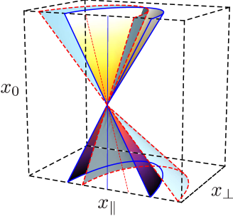
Figure 1: Null cone of the standard theory (blue, solid lines) and one of the modified null cones (red, dashed lines) in configuration space $(x_{0},x_{\bot},x_{\parallel})$. Their rotation axes are shown as well (thin lines).

Since there are two modes with two different dispersion relations, one may wonder, if this result is sufficient for taking a decision about microcausality. For this reason we tried to separate both modes in Sec. IV with the result (4.8) – (4.10). Therefore, we should investigate $\widehat{G}^{(1)}(k)$ and $\widehat{G}^{(2)}(k)$ from Eq. (4.10):

$$\widehat{G}^{(1)}(x) \equiv\oint_{C}\frac{\mathrm{d}k_{0}}{2\pi}\int\frac{\mathrm{d}^{3}k}{(2\pi)^{3}}\widehat{G}^{(1)}(k)$$

$$=\oint_{C}\frac{\mathrm{d}k_{0}}{2\pi}\int\frac{\mathrm{d}^{3}k}{(2\pi)^{3}}\,\frac{4\widehat{K}_{1}\widehat{K}_{2}^{-1}}{[(k\cdot\xi)^{2}-k^{2}]\zeta^{2}+(k\cdot\zeta)^{2}}\exp(\mathrm{i}\,k_{0}x_{0}+\mathrm{i}\,\mathbf{k}\cdot\mathbf{x})$$

$$=\oint_{C}\frac{\mathrm{d}k_{0}}{2\pi}\int\frac{\mathrm{d}^{3}k}{(2\pi)^{3}}\,\frac{4\widehat{K}_{2}^{-1}}{[(k\cdot\xi)^{2}-k^{2}]\zeta^{2}+(k\cdot\zeta)^{2}}\frac{\exp(\mathrm{i}\,k_{0}x_{0}+\mathrm{i}\,\mathbf{k}\cdot\mathbf{x})}{(k_{0}-\widetilde{\omega}_{1}^{+})(k_{0}-\widetilde{\omega}_{1}^{-})}\,.$$ (7.9)

Using

$$\left.\frac{4\widehat{K}_{2}^{-1}}{[(k\cdot\xi)^{2}-k^{2}]\zeta^{2}+(k\cdot\zeta)^{2}}\right|_{k_{0}=\widetilde{\omega}_{1}^{+}}=\left.\frac{4\widehat{K}_{2}^{-1}}{[(k\cdot\xi)^{2}-k^{2}]\zeta^{2}+(k\cdot\zeta)^{2}}\right|_{k_{0}=\widetilde{\omega}_{1}^{-}}=1\,,$$ (7.10)

then leads to the intermediate result of Eq. (VII) and the rest of the computation is the same. Since $\widehat{G}^{(2)}(k)$ is a constant function with respect to $k_{0}$, the evaluation of the contour integral in the complex $k_{0}$-plane in

$$\widehat{G}^{(2)}(x)\equiv\oint_{C}\frac{\mathrm{d}k_{0}}{2\pi}\int\frac{\mathrm{d}^{3}k}{(2\pi)^{3}}\widehat{G}^{(2)}(k)\,,$$ (7.11)

will immediately give zero. Hence, the dispersion relation corresponding to the second mode does not seem to play any role here. The $\lambda=1$ mode seems to be preferred compared to the $\lambda=2$ mode, what follows from forcing a parity-odd theory to be nonbirefringent via the Ansatz (2.2). The transversal polarization vectors can be interpreted as two distinct polarization modes: left- and right-handed. In a parity-violating theory they are expected to behave differently, for example with respect to their phase velocity. This would automatically lead to birefringence, which is suppressed by using Eq. (2.2) as a basis.

The result of Eq. (VII) establishes microcausality for the following parameter domain:

$$\mathcal{E}\equiv|\boldsymbol{\zeta}|\in[0,\,\infty)\,,$$ (7.12)

where $\boldsymbol{\zeta}$ is defined in terms of the SME parameters by Eqs. (2.3b) and (2.4). Hence, the parity-odd “nonbirefringent” sector of modified Maxwell theory is unitary and microcausal for the full parameter range.

VIII Comparison to other Lorentz-violating theories

In the previous sections we have seen that both the modified photon propagator and the polarization vectors have an uncommon structure. For this reason, we want to have a general look at the photon propagator and polarization vectors in other Lorentz-violating theories. We start with the photon polarizations of MCS theory. Besides modified Maxwell theory, MCS theory is another possible example of a gauge-invariant and power-counting renormalizable theory that violates Lorentz invariance in the photon sector. MCS theory is characterized by a mass scale $m_{\scriptscriptstyle{\mathrm{CS}}}$ and a fixed spacelike “four-vector” $\zeta^{\mu}$, that plays the role of a background field. The Chern–Simons mass $m_{\scriptscriptstyle{\mathrm{CS}}}$ gives the amount of Lorentz violation. MCS theory exhibits two photon modes, which we call ‘$\oplus$’ and ‘$\ominus$’. They obey different dispersion relations Carroll-etal1990 , which results in birefringence. The polarization vectors follow from the field equations and, in temporal gauge $A^{0}=0$, they are given by

$$(\varepsilon^{\oplus\,\mu})=\frac{1}{\sqrt{N^{\prime}}}\left(0\,,\,-2[(k\cdot\zeta)^{2}+k^{2}]\,,\,\mathrm{i}\frac{2\omega}{m_{\mathrm{\scriptscriptstyle{CS}}}}k^{2}\,,\,2k_{\parallel}k_{\bot}\right)\Bigg{|}_{\omega=\omega_{\oplus}}\,,$$ (8.1a)

$$(\varepsilon^{\ominus\,\mu})=\frac{1}{\sqrt{N^{\prime\prime}}}\left(0\,,\,-2[(k\cdot\zeta)^{2}+k^{2}]\,,\,\mathrm{i}\frac{2\omega}{m_{\mathrm{\scriptscriptstyle{CS}}}}k^{2}\,,\,2k_{\parallel}k_{\bot}\right)\Bigg{|}_{\omega=\omega_{\ominus}}\,,$$ (8.1b)

with the normalization constants

$$N^{\prime}=4\frac{\omega^{2}k^{2}}{m^{2}_{\mathrm{\scriptscriptstyle{CS}}}}[2k^{2}+m^{2}_{\mathrm{\scriptscriptstyle{CS}}}\zeta^{2}]\Big{|}_{\omega=\omega_{\oplus}}\,,\quad N^{\prime\prime}=4\frac{\omega^{2}k^{2}}{m^{2}_{\mathrm{\scriptscriptstyle{CS}}}}[2k^{2}+m^{2}_{\mathrm{\scriptscriptstyle{CS}}}\zeta^{2}]\Big{|}_{\omega=\omega_{\ominus}}\,.$$ (8.1c)

Using the temporal gauge fixing four-vector $(n^{\mu})=(1,0,0,0)$, the polarization tensor for each of the two modes can be cast in the following form (see Kaufhold:2005vj for the truncated versions):

$$\overline{\varepsilon}^{\oplus\,\mu}(k)\varepsilon^{\oplus\,\nu}(k)=\Pi^{\mu\nu}_{\mathrm{MCS}}\big{|}_{\omega=\omega_{\oplus}}\,,$$ (8.2a)

$$\overline{\varepsilon}^{\ominus\,\mu}(k)\varepsilon^{\ominus\,\nu}(k)=\Pi^{\mu\nu}_{\mathrm{MCS}}\big{|}_{\omega=\omega_{\ominus}}\,,$$ (8.2b)

where

$$\Pi^{\mu\nu}_{\mathrm{MCS}} =\frac{1}{2k^{2}+m_{\mathrm{\scriptscriptstyle{CS}}}^{2}\zeta^{2}}\left[-\,k^{2}\eta^{\mu\nu}-\frac{k^{2}}{(k\cdot n)^{2}}k^{\mu}k^{\nu}+\frac{k^{2}}{k\cdot n}(k^{\mu}n^{\nu}+n^{\mu}k^{\nu})\right.$$

$$\phantom{{}={}\frac{1}{2k^{2}+m_{\mathrm{\scriptscriptstyle{CS}}}^{2}\zeta^{2}}\Big{[}}\left.-\,m_{\mathrm{\scriptscriptstyle{CS}}}^{2}\zeta^{\mu}\zeta^{\nu}-\mathrm{i}m_{\mathrm{\scriptscriptstyle{CS}}}\varepsilon^{\mu\nu\varrho\sigma}\left(\frac{k\cdot\zeta}{k\cdot n}k_{\varrho}n_{\sigma}-\frac{k^{2}}{k\cdot n}\zeta_{\varrho}n_{\sigma}\right)\right]\,.$$ (8.2c)

The polarization sum of standard QED is expected to be recovered for vanishing $m_{\scriptscriptstyle{\mathrm{CS}}}$. For the truncated polarization sum this is, indeed, the case:

$$\lim_{m_{\scalebox{0.4}{CS}}\mapsto 0}\left.\Big{\{}\overline{\varepsilon}^{\oplus\,\mu}(k)\varepsilon^{\oplus\,\nu}(k)+\overline{\varepsilon}^{\ominus\,\mu}(k)\varepsilon^{\ominus\,\nu}(k)\Big{\}}\right|^{\text{truncated}}=-\eta^{\mu\nu}\,.$$ (8.3)

From

$$\lim_{m_{\scalebox{0.4}{CS}}\mapsto 0}\overline{\varepsilon}^{\oplus\,\mu}(k)\varepsilon^{\oplus\,\nu}(k)\,\Big{|}^{\text{truncated}}=\lim_{m_{\scalebox{0.4}{CS}}\mapsto 0}\overline{\varepsilon}^{\ominus\,\mu}(k)\varepsilon^{\ominus\,\nu}(k)\,\Big{|}^{\text{truncated}}=-\frac{\eta^{\mu\nu}}{2}\,,$$ (8.4)

it is evident that both modes deliver equal contributions to the polarization sum. This even holds for nonvanishing $m_{\scriptscriptstyle{\mathrm{CS}}}$. Hence, the behavior of MCS theory with respect to the polarization modes is completely different compared to parity-odd nonbirefringent modified Maxwell theory. For $m_{\scriptscriptstyle{\mathrm{CS}}}\mapsto 0$, there is no residual dependence from the preferred spacetime direction $\zeta^{\mu}$ in the polarization tensors of the individual modes, which can be seen from Eq. (8.4).

Furthermore, for MCS-theory the photon propagator in the axial gauge has been shown to be of the following form AdamKlinkhamer2001 :

$$G_{\mu\nu}(k)\Big{|}^{\mathrm{axial}}_{\mathrm{MCS}}=-\mathrm{i}\frac{k^{2}}{\mathscr{P}(k)}\left(\eta_{\mu\nu}+\ldots\right)\,,$$ (8.5)

where further terms with the index structure composed of the four-momentum, the preferred spacelike four-vector $\zeta^{\mu}$, the axial gauge vector and the four-dimensional Levi-Civita symbol have been omitted. The denominator $\mathscr{P}(k)$ is a fourth-order polynomial in $k^{0}$, with its zeros corresponding to the two different physical dispersion relations. For a special case of parity-odd ‘birefringent’ modified Maxwell theory we could show that the propagator in Feynman gauge looks like

$$G_{\mu\nu}(k)\Big{|}^{\mathrm{Feynman}}_{\begin{subarray}{c}\mathrm{birefringent}\\ \mathrm{modMax}\hfill\end{subarray}}=-\mathrm{i}\frac{\mathscr{P}_{1}(k)}{\mathscr{P}_{2}(k)}\left(\eta_{\mu\nu}+\ldots\right)\,,$$ (8.6)

where $\mathscr{P}_{1}(k)$ is a second-order polynomial in $k^{0}$, involving the Lorentz-violating parameters and $\mathscr{P}_{2}(k)$ is of fourth order in $k^{0}$. The two distinct physical dispersion relations of this birefringent theory follow from $\mathscr{P}_{2}(k)=0$. Again, remaining propagator coefficients multiplied by combinations of the four-momentum and preferred four-vectors have been omitted.

Hence, we see that our result for the propagator for parity-odd nonbirefringent modified Maxwell theory given by Eqs. (IV) – (4.5) is rather unusual. For MCS-theory and birefringent modified Maxwell theory (at least for the special case examined), both physical modes emerge as poles of the coefficient before the metric tensor $\eta_{\mu\nu}$. However, in the case of parity-odd nonbirefringent modified Maxwell theory, the dispersion relation for the $\lambda=2$ polarization mode is not contained in the coefficient $\widehat{K}_{1}$ of Eq. (4.4a), which is multiplied with $\eta_{\mu\nu}$. This peculiarity is also mirrored in the polarization tensors, where we have shown the interplay in the previous section.

IX Limit of the polarization tensors for vanishing Lorentz violation

Taking the limit $\mathcal{E}\mapsto 0$ followed by the limit $k_{\bot}\mapsto 0$ (see the definition (3.4)) for the physical polarization vectors (5.1) and (5.2) leads to:

$$\lim_{\begin{subarray}{c}\mathcal{E}\mapsto 0\\ k_{\bot}\mapsto 0\end{subarray}}(\varepsilon^{(1)\,\mu})=\begin{pmatrix}0\\ 0\\ 1\\ 0\\ \end{pmatrix}\,,\quad\lim_{\begin{subarray}{c}\mathcal{E}\mapsto 0\\ k_{\bot}\mapsto 0\end{subarray}}(\varepsilon^{(2)\,\mu})=\begin{pmatrix}0\\ 1\\ 0\\ 0\\ \end{pmatrix}\,.$$ (9.1)

Taking into account the limit of the four-momentum,

$$\lim_{k_{\bot}\mapsto 0}\begin{pmatrix}k_{\bot}\\ 0\\ k_{\parallel}\\ \end{pmatrix}=\begin{pmatrix}0\\ 0\\ k_{\parallel}\\ \end{pmatrix}\equiv\begin{pmatrix}0\\ 0\\ k\\ \end{pmatrix}\,,$$ (9.2)

the physical polarization vectors reduce to the standard transversal QED results. Note that for both vectors in Eq. (9.1), the order in which the limits are taken does not play any role. As we will see below, this is not the case for the gauge-invariant parts of the polarization tensors from Eqs. (5.6), (5.9), that is, if the polarization vectors are coupled to conserved currents. For $\mathcal{E}\mapsto 0$ these tensors result in:

$$\lim_{\mathcal{E}\mapsto 0}\Pi^{\mu\nu}|_{\lambda=1}=-\eta^{\mu\nu}-\frac{k_{\parallel}^{2}}{k_{\bot}^{2}}\xi^{\mu}\xi^{\nu}-\frac{|\mathbf{k}|^{2}}{k_{\bot}^{2}}\widehat{\zeta}^{\mu}\widehat{\zeta}^{\nu}-\frac{|\mathbf{k}|k_{\parallel}}{k_{\bot}^{2}}(\xi^{\mu}\widehat{\zeta}^{\nu}+\xi^{\nu}\widehat{\zeta}^{\mu})\,,$$ (9.3a)

$$\lim_{\mathcal{E}\mapsto 0}\Pi^{\mu\nu}|_{\lambda=2}=\frac{k_{\parallel}^{2}}{k_{\bot}^{2}}\xi^{\mu}\xi^{\nu}+\frac{|\mathbf{k}|^{2}}{k_{\bot}^{2}}\widehat{\zeta}^{\mu}\widehat{\zeta}^{\nu}+\frac{|\mathbf{k}|k_{\parallel}}{k_{\bot}^{2}}(\xi^{\mu}\widehat{\zeta}^{\nu}+\xi^{\nu}\widehat{\zeta}^{\mu})\,,$$ (9.3b)

with $(\widehat{\zeta}^{\mu})=(0,\widehat{\boldsymbol{\zeta}})$ and $|\mathbf{k}|=(k_{\scriptscriptstyle{\parallel}}^{2}+k_{\bot}^{2})^{1/2}$. For completeness, after inserting the explicit four-vectors, we obtain the following matrices:

$$\lim_{\mathcal{E}\mapsto 0}\big{(}\Pi^{\mu\nu}|_{\lambda=1}\big{)} =\frac{1}{k_{\bot}^{2}}\begin{pmatrix}-|\mathbf{k}|^{2}&0&0&-|\mathbf{k}|k_{\parallel}\\ 0&k_{\bot}^{2}&0&0\\ 0&0&k_{\bot}^{2}&0\\ -|\mathbf{k}|k_{\parallel}&0&0&-k_{\parallel}^{2}\\ \end{pmatrix}\,,$$ (9.4a)

$$\lim_{\mathcal{E}\mapsto 0}\big{(}\Pi^{\mu\nu}|_{\lambda=2}\big{)}=\frac{1}{k_{\bot}^{2}}\begin{pmatrix}k_{\parallel}^{2}&0&0&|\mathbf{k}|k_{\parallel}\\ 0&0&0&0\\ 0&0&0&0\\ |\mathbf{k}|k_{\parallel}&0&0&|\mathbf{k}|^{2}\\ \end{pmatrix}\,.$$ (9.4b)

Note that these matrix representations only hold for the special choice $\widehat{\boldsymbol{\zeta}}=(0,0,1)$. It is evident that the additional limit $k_{\bot}\mapsto 0$ does not exist for each contribution $\Pi^{\mu\nu}|_{\lambda=1}$ or $\Pi^{\mu\nu}|_{\lambda=2}$ separately, but only for the truncated polarization sum $\sum_{\lambda=1,2}\Pi^{\mu\nu}|_{\lambda}$, which leads to the standard QED result. For this reason, the polarization vectors are not only deformed — unlike for the isotropic case that was examined in Ref. Klinkhamer:2010zs — but their structure completely differs from standard QED. Besides that, no covariant expression exists for each polarization tensor in standard QED, where only the sum $\sum_{\lambda=1,2}\Pi^{\mu\nu}|_{\lambda}$ can be decomposed covariantly.

X Physical process: Compton scattering with polarized photons

X.1 Description of the process

The results obtained for the polarization vectors in Sec. V together with the observations that followed forces us to think about the consistency of the modified theory. The form of the propagator, the polarization vectors and tensors observed in Secs. IV, V, and IX reveal the following uncommon properties:

• one of the two physical photon modes seems to be preferred with respect to the other,

• both polarization vectors are interweaved with the spacetime directions $\xi^{\mu}$ and $\zeta^{\mu}$, even for vanishing Lorentz-violating parameters,

• each physical polarization tensor can be written in covariant form,

• and one of the physical polarization vectors has a longitudinal part.

One the one hand, these peculiarities may emerge from the fact that a parity-odd QED is combined with the claim of being nonbirefringent. Two physical photon polarizations can be interpreted as two distinct polarization modes:“left-handed” and “right-handed”. These are supposed to behave differently because of parity violation, for example with respect to the phase velocity of each mode. Hence, birefringence would result from this, which clashes with the nonbirefringent Ansatz of Eq. (2.2).

On the other hand, the above properties may have emerged from a bad gauge choice and could possibly be removed by picking a more appropriate gauge. For this reason a physical process will be considered, whose cross section does not depend on the gauge. If the mentioned behavior of the polarization modes is not a gauge artifact, it will show up in the results for polarized cross sections. The simplest tree-level process involving external photons, which also occurs in standard QED, is Compton scattering. We consider an electron scattered off a photon in the $\lambda=1$ polarization and in the $\lambda=2$ polarization, respectively. Hence, we want to compute cross sections for the processes $e^{-}(p_{1})\widetilde{\gamma}_{1}(k_{1})\rightarrow e^{-}(p_{2})\widetilde{\gamma}_{1}(k_{2})$, $e^{-}(p_{1})\widetilde{\gamma}_{1}(k_{1})\rightarrow e^{-}(p_{2})\widetilde{\gamma}_{2}(k_{2})$, $e^{-}(p_{1})\widetilde{\gamma}_{2}(k_{1})\rightarrow e^{-}(p_{2})\widetilde{\gamma}_{1}(k_{2})$, and $e^{-}(p_{1})\widetilde{\gamma}_{2}(k_{1})\rightarrow e^{-}(p_{2})\widetilde{\gamma}_{2}(k_{2})$, where $\widetilde{\gamma}_{1,2}$ denotes a modified photon in the $\lambda=1$ or $\lambda=2$ polarization state, respectively. The corresponding Feynman diagrams are shown in Fig. 2.

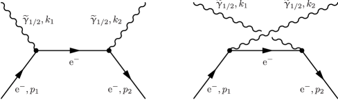
Figure 2: Contributions to Compton scattering for polarized modified photons $\widetilde{\gamma}_{1,2}$, where the subscript refers to the photon polarization. The photon momenta are denoted as $k_{a}$ and the electron momenta as $p_{a}$, where the label $a=1$, 2 refers to the initial and final state, respectively.

For a review of Compton scattering experiments, refer to Ref. Fluegge1958 . Furthermore, Ref. Bocquet:2010ke gives a new bound on two of the three parameters of parity-odd nonbirefringent modified Maxwell theory from the study of Compton scattering kinematics at the GRAAL experiment on the European Synchrotron Radiation Facility (ESRF) at Grenoble in France.

X.2 Numerical results for polarized Compton scattering cross sections

We choose special momenta $p_{1}$, $k_{1}$ for the initial electron and photon. The outgoing photon momentum configuration is described in spherical coordinates with polar angle $\vartheta$ and azimuthal angle $\varphi$. We consider the initial momentum configuration, for which the electron is at rest: $(p_{1}^{\mu})=(m,0,0,0)$, $(k_{1,\lambda}^{\mu})\equiv(\omega_{\lambda}(k),\mathbf{k})$ with $\mathbf{k}=(0,0,|\mathbf{k}|)=(0,0,k_{1})$.

$k_{1}/m$	$10^{-1}$	$10^{-2}$	$10^{-3}$	$10^{-4}$	$10^{-5}$
$\sigma$	7.048378	8.214276	8.360869	8.375905	8.377413
$k_{1}/m$	$10^{-6}$	$10^{-7}$	$10^{-8}$	$10^{-9}$	$10^{-10}$
$\sigma$	8.377564	8.377579	8.377580	8.377580	8.377580

Table 1: Unpolarized total Compton scattering cross sections $\sigma$ in standard QED for different values of the initial photon momentum $k_{1}$ according to the equation below (5-114) of ItzyksonZuber1980 or to Eq. (5.81) of PeskinSchroeder1995 . The results are given in units of $\alpha^{2}$ with the fine structure constant $\alpha\equiv e^{2}/4\pi$. The electron mass is set to $m=1$.

$k_{1}/m$	$\sigma_{11}$	$\sigma_{22}$	$\sigma_{12}$	$\sigma_{21}$	$\sum_{\lambda^{\prime}}\sigma_{1\lambda^{\prime}}$	$\sum_{\lambda^{\prime}}\sigma_{2\lambda^{\prime}}$	$\frac{1}{2}\sum_{\lambda,\lambda^{\prime}}\sigma_{\lambda\lambda^{\prime}}$
$10^{-1}$	1.784650	5.263729	5.263729	1.784650	7.048379	7.048379	7.048379
$10^{-2}$	2.053890	6.160386	6.160386	2.053890	8.214277	8.214277	8.214277
$10^{-3}$	2.090221	6.270648	6.270648	2.090221	8.360869	8.360869	8.360869
$10^{-4}$	2.093976	6.281929	6.281929	2.093976	8.375905	8.375905	8.375905
$10^{-5}$	2.094353	6.283060	6.283060	2.094353	8.377413	8.377413	8.377413

Table 2: Polarized Compton scattering cross sections $\sigma_{\lambda\lambda^{\prime}}$ (where $\lambda$ denotes the initial and $\lambda^{\prime}$ the final photon polarization) of standard QED for different values of the initial photon momentum $k_{1}$ according to Eq. (11-13) of JauchRohrlich1976 . The cross sections are given in units of $\alpha^{2}$ and the electron mass is set to $m=1$.

$\widetilde{\kappa}$	$\widetilde{\sigma}_{11}$	$\widetilde{\sigma}_{22}$	$\widetilde{\sigma}_{12}$	$\widetilde{\sigma}_{21}$	$\widetilde{\sigma}_{1X}$	$\widetilde{\sigma}_{2X}$	$\widetilde{\sigma}$
$10^{-1}$	6.283180	5.526582	2.033397	2.890066	8.316577	8.416647	8.366612
	6.283180	5.526586	2.033399	2.890066	8.316579	8.416652	8.366615
$10^{-2}$	6.283180	6.200243	2.093772	2.177939	8.376952	8.378182	8.377567
	6.283180	6.200245	2.093772	2.177939	8.376952	8.378184	8.377568
$10^{-4}$	6.283180	6.282133	2.094338	2.095235	8.377518	8.377367	8.377443
	6.283180	6.282346	2.094400	2.095235	8.377580	8.377581	8.377581
$10^{-8}$	6.283175	6.282743	2.094270	2.094397	8.377444	8.377140	8.377292
	6.283180	6.283184	2.094400	2.094397	8.377580	8.377581	8.377580
$10^{-16}$	6.283180	6.283258	2.094400	2.094397	8.377581	8.377655	8.377618
	6.283180	6.283184	2.094400	2.094397	8.377581	8.377581	8.377581

Table 3: Compton scattering cross sections $\widetilde{\sigma}_{\lambda\lambda^{\prime}}$ for polarized modified photons, where $\lambda$ is the initial and $\lambda^{\prime}$ the final photon mode. The sixth and seventh columns give the combinations defined by Eq. (10.1) and the eighth column lists the sum of the four cross sections $\widetilde{\sigma}_{\lambda\lambda^{\prime}}$, which is averaged over the initial photon polarizations and corresponds to the cross section of unpolarized modified Compton scattering from Eq. (10.2). The electrons are assumed to be unpolarized. All results are given in units of $\alpha^{2}$ and $k_{1}=10^{-10}m$ is used. Moreover, we set the electron mass $m=1$. The Lorentz-violating parameter $\widetilde{\kappa}$ can be found in the first column. For each Lorentz-violating parameter we give both the results that follow from Eq. (10.3) (first row) and from Eq. (10.5) (second row), respectively.

$k_{1}/m$	$\widetilde{\sigma}_{11}$	$\widetilde{\sigma}_{22}$	$\widetilde{\sigma}_{12}$	$\widetilde{\sigma}_{21}$	$\widetilde{\sigma}_{1X}$	$\widetilde{\sigma}_{2X}$	$\widetilde{\sigma}$
$10^{-1}$	5.278215	5.280137	1.770163	1.768241	7.048378	7.048378	7.048378
	5.278215	5.280137	1.770163	1.768241	7.048378	7.048378	7.048378
$10^{-2}$	6.160582	6.160613	2.053694	2.053664	8.214277	8.214277	8.214277
	6.160582	6.160613	2.053694	2.053664	8.214277	8.214277	8.214277
$10^{-3}$	6.270645	6.270649	2.090224	2.090220	8.360869	8.360869	8.360869
	6.270645	6.270649	2.090224	2.090220	8.360869	8.360869	8.360869
$10^{-4}$	6.281924	6.281927	2.093982	2.093978	8.375905	8.375905	8.375905
	6.281924	6.281927	2.093982	2.093978	8.375905	8.375905	8.375905
$10^{-5}$	6.283054	6.283058	2.094359	2.094355	8.377413	8.377413	8.377413
	6.283054	6.283058	2.094359	2.094355	8.377413	8.377413	8.377413

Table 4: Modified polarized Compton scattering cross sections $\widetilde{\sigma}_{\lambda\lambda^{\prime}}$ in units of $\alpha^{2}$ for fixed Lorentz-violating parameter $\widetilde{\kappa}=10^{-16}$, where $\lambda$ is the initial and $\lambda^{\prime}$ the final photon polarization. The cross sections are computed for different values of the initial photon momentum $k_{1}$. As before, for each $k_{1}$ the first row gives the results that follow by using $X_{\lambda\lambda^{\prime}}$ from Eq. (10.3). The second row delivers the corresponding result $\widehat{X}_{\lambda\lambda^{\prime}}$ from Eq. (10.5).

$\widetilde{\kappa}^{01}$	$\widetilde{\kappa}^{02}$	$\widetilde{\kappa}^{03}$	$\widetilde{\sigma}_{11}$	$\widetilde{\sigma}_{22}$	$\widetilde{\sigma}_{12}$	$\widetilde{\sigma}_{21}$	$\widetilde{\sigma}_{1X}$	$\widetilde{\sigma}_{2X}$	​​$\widetilde{\sigma}$
1	1	2	6.283177	4.188794	2.094403	4.188795	8.377581	8.377590	8.377585
1	2	1	6.281280	7.330112	2.096301	1.047515	8.377581	8.377627	8.377604
			6.281280	7.330065	2.096301	1.047515	8.377581	8.377581	8.377581
2	1	1	6.281280	7.330112	2.096301	1.047515	8.377581	8.377627	8.377604
1	1	3	6.282966	3.236618	2.094614	5.140967	8.377581	8.377585	8.377583
1	3	1	6.281874	7.806356	2.095706	0.571318	8.377581	8.377674	8.377627
3	1	1	6.281874	7.806356	2.095706	0.571318	8.377581	8.377674	8.377627
1	1	5	6.283181	2.559814	2.094399	5.817768	8.377581	8.377582	8.377581
1	5	1	6.280175	8.145009	2.097405	0.232822	8.377581	8.377831	8.377706
5	1	1	6.280175	8.145009	2.097405	0.232822	8.377581	8.377831	8.377706
1	1	10	6.283322	2.217729	2.094258	6.159851	8.377581	8.377581	8.377581
1	10	1	6.285520	8.317100	2.092061	0.061577	8.377581	8.378677	8.378129
10	1	1	6.285520	8.317100	2.092061	0.061577	8.377581	8.378677	8.378129
10	1	10	6.281734	5.235428	2.095847	3.142161	8.377581	8.377590	8.377585

Table 5: Cross sections of modified polarized Compton scattering in units of $\alpha^{2}$ for different values of $\widetilde{\kappa}^{01}$, $\widetilde{\kappa}^{02}$, and $\widetilde{\kappa}^{03}$, where the latter parameters are given in magnitudes of $10^{-16}$. In the second row we also give the result that follows $\widehat{X}_{\lambda\lambda^{\prime}}$. The photon momentum is $k_{1}=10^{-10}m$.

Values for the modified polarized Compton scattering cross sections $\widetilde{\sigma}_{11}$, $\widetilde{\sigma}_{12}$, $\widetilde{\sigma}_{21}$, and $\widetilde{\sigma}_{22}$ are obtained. These correspond to the processes $1\mapsto 1$, $1\mapsto 2$, $2\mapsto 1$, and $2\mapsto 2$, where the numbers give the initial and final photon polarization, respectively. To form gauge-invariant expressions, the sum over final photon polarizations has to be performed:

$$\widetilde{\sigma}_{1X}\equiv\sum_{\lambda^{\prime}=1,2}\widetilde{\sigma}_{1\lambda^{\prime}}\,,$$ (10.1a)

$$\widetilde{\sigma}_{2X}\equiv\sum_{\lambda^{\prime}=1,2}\widetilde{\sigma}_{2\lambda^{\prime}}\,.$$ (10.1b)

Our calculation is based on the assumption that only the initial photon state can be prepared, especially its polarization. However, the final photon polarization can only be measured, if the photon is observed or scattered at a second electron. Since we consider the final photon as an asymptotic particle according to the Feynman diagrams in Fig. 2, it is not observed and one has to sum over final photon polarizations PeskinSchroeder1995 ; ItzyksonZuber1980 . Hence, what can be measured in this context are only the quantities $\widetilde{\sigma}_{1X}$ and $\widetilde{\sigma}_{2X}$, so we also give them.

Finally, we list the sum of all cross sections, which is averaged over the initial photon polarizations:

$$\widetilde{\sigma}\equiv\frac{1}{2}\sum_{\lambda,\lambda^{\prime}}\widetilde{\sigma}_{\lambda\lambda^{\prime}}=\frac{1}{2}(\widetilde{\sigma}_{11}+\widetilde{\sigma}_{12}+\widetilde{\sigma}_{21}+\widetilde{\sigma}_{22})=\frac{1}{2}(\widetilde{\sigma}_{1X}+\widetilde{\sigma}_{2X})\,.$$ (10.2)

For comparison with the modified Compton cross sections, the cross sections for unpolarized and polarized Compton scattering in standard QED are presented in Table 1 and Table 2, respectively, for different initial photon momenta $k_{1}$.

An important issue has to be mentioned first: the calculation of the modified cross section in the parity-odd theory can be performed in two different ways. The first possibility is to calculate the matrix element squared à la Sec. (11.1) of Ref. JauchRohrlich1976 by directly using the modified polarization vectors from Eqs. (5.1), (5.2). For completeness, we give this equation in a compact form:

$$X_{\lambda\lambda^{\prime}} =\frac{1}{4}\mathrm{Tr}\left\{\left[\frac{1}{\upsilon_{1}}\cancel{\varepsilon}^{(\lambda^{\prime})}(\cancel{p}_{1}+\cancel{k}_{1}+m)\cancel{\varepsilon}^{(\lambda)}-\frac{1}{\upsilon_{2}}\cancel{\varepsilon}^{(\lambda)}(\cancel{p}_{1}-\cancel{k}_{2}+m)\cancel{\varepsilon}^{(\lambda^{\prime})}\right](\cancel{p}_{1}+m)\right.$$

$$\phantom{{}={}\frac{1}{4}\mathrm{Tr}}\left.\times\left[\frac{1}{\upsilon_{1}}\cancel{\varepsilon}^{(\lambda)}(\cancel{p}_{1}+\cancel{k}_{1}+m)\cancel{\varepsilon}^{(\lambda^{\prime})}-\frac{1}{\upsilon_{2}}\cancel{\varepsilon}^{(\lambda^{\prime})}(\cancel{p}_{1}-\cancel{k}_{2}+m)\cancel{\varepsilon}^{(\lambda)}\right](\cancel{p}_{2}+m)\right\}\,,$$ (10.3a)

where

$$\upsilon_{1}=2p_{1}\cdot k_{1}+k_{1}^{2}\,,\quad\upsilon_{2}=2p_{1}\cdot k_{2}-k_{2}^{2}\,,\quad p_{2}=p_{1}+k_{1}-k_{2}\,.$$ (10.3b)

Here, $\lambda$ denotes the initial and $\lambda^{\prime}$ the final photon polarization. For standard QED Eq. (10.3) results in Eq. (11-13) of Ref. JauchRohrlich1976 (which we transform to fit our conventions):

$$X_{\lambda\lambda^{\prime}}^{\mathrm{QED}} =\frac{1}{2}\left(\frac{\upsilon}{\upsilon^{\prime}}+\frac{\upsilon^{\prime}}{\upsilon}\right)-1$$

$$\phantom{{}=\frac{1}{2}{}}+2\left[\varepsilon^{(\lambda)}\cdot\varepsilon^{(\lambda^{\prime})}-\frac{2(\varepsilon^{(\lambda)}\cdot p_{1})(\varepsilon^{(\lambda^{\prime})}\cdot p_{2})}{\upsilon}+\frac{2(\varepsilon^{(\lambda)}\cdot p_{2})(\varepsilon^{(\lambda^{\prime})}\cdot p_{1})}{\upsilon^{\prime}}\right]^{2}\,,$$ (10.4a)

$$\upsilon=2p_{1}\cdot k_{1}\,,\quad\upsilon^{\prime}=2p_{1}\cdot k_{2}\,.$$ (10.4b)

Alternatively, the computation can be performed with the matrix element squared that is obtained without the direct use of the polarization vectors, but with the polarization tensors from Eqs. (V), (V). This expression is lengthy and we will not give it in full detail. However, we will state it in a formal manner:

$$\widehat{X}_{\lambda\lambda^{\prime}}=\big{(}|\mathcal{M}(k_{1},k_{2})|^{2}\big{)}^{\mu\nu\varrho\sigma}\Pi_{\mu\varrho}(k_{1})|_{\lambda}\Pi_{\nu\sigma}(k_{2})|_{\lambda^{\prime}}\Big{|}_{\begin{subarray}{c}k_{1}^{0}=\omega_{\lambda}(\mathbf{k}_{1})\\ k_{2}^{0}=\omega_{\lambda^{\prime}}(\mathbf{k}_{2})\end{subarray}}\,,$$ (10.5)

where $\Pi_{\mu\nu}$ are photon polarization tensors and $\big{(}|\mathcal{M}(k_{1},k_{2})|^{2}\big{)}^{\mu\nu\varrho\sigma}$ includes all parts that do not directly involve the photon: traces of combinations of $\gamma$-matrices, electron propagators etc. The structure of $\widehat{X}_{\lambda\lambda^{\prime}}$ is similar to Eq. (5.81) of Ref. PeskinSchroeder1995 . However, the latter equation gives the sum over all polarizations, whereas $\widehat{X}_{\lambda\lambda^{\prime}}$ is the amplitude square for a distinct polarization.

For the configurations of Table 3 and 4 the results are shown for different Lorentz-violating parameters $\widetilde{\kappa}$, where $\widetilde{\kappa}$ is defined by $\widetilde{\kappa}\equiv\mathcal{E}/\sqrt{3}$ with $\mathcal{E}$ of Eq. (3.5c). It suffices to give $\widetilde{\kappa}$, since for both tables the three Lorentz-violating parameters $\widetilde{\kappa}^{01}$, $\widetilde{\kappa}^{02}$, and $\widetilde{\kappa}^{03}$ are chosen to be equal. Table 5 presents results, where the latter parameters differ from each other. Compare the obtained results to the classical Thomson cross section, which follows from the standard QED result — first obtained by Klein and Nishina — in the limit of vanishing initial photon momentum PeskinSchroeder1995 :

$$\sigma^{\mathrm{Th}}\equiv\lim_{\begin{subarray}{c}|\mathbf{k}_{1}|\mapsto 0\\ |\mathbf{p}_{1}|\mapsto 0\end{subarray}}\sigma\big{(}e^{-}(p_{1})\gamma(k_{1})\rightarrow e^{-}(p_{2})\gamma(k_{2})\big{)}=\frac{8\pi\alpha^{2}}{3m^{2}}\approx\frac{8.377580\alpha^{2}}{m^{2}}\,.$$ (10.6)

From Table 3 we see that for vanishing Lorentz violation the gauge-invariant contributions from Eq. (10.1) are equal:

$$\lim_{\widetilde{\kappa}\mapsto 0}\widetilde{\sigma}_{1X}=\lim_{\widetilde{\kappa}\mapsto 0}\widetilde{\sigma}_{2X}\,.$$ (10.7)

Furthermore, the sum of all cross sections then corresponds to the Thomson limit given in Eq. (10.6). The results for $\widetilde{\sigma}_{11}$, $\widetilde{\sigma}_{12}$, and $\widetilde{\sigma}_{21}$ do not depend on whether Eq. (10.3) or Eq. (10.5) is used for the calculation.

From Table 4 it also follows that, for vanishing Lorentz violation, $\widetilde{\sigma}_{1X}=\widetilde{\sigma}_{2X}$ and, furthermore, that the averaged sum over all cross sections corresponds to the standard Klein–Nishina results. Besides, all results are independent of the fact of whether the calculation is based on $X_{\lambda\lambda^{\prime}}$ or $\widehat{X}_{\lambda\lambda^{\prime}}$. This is also the case for the first selection of parameters in Table 5. Furthermore, this table shows that the individual cross sections $\widetilde{\sigma}_{11}$, $\widetilde{\sigma}_{12}$, $\widetilde{\sigma}_{21}$, and $\widetilde{\sigma}_{22}$ depend on the direction of $\boldsymbol{\zeta}$, which is encoded in the choice of $\widetilde{\kappa}^{01}$, $\widetilde{\kappa}^{02}$, and $\widetilde{\kappa}^{03}$. However, it is evident that the gauge-invariant expressions defined in Eq. (10.1) are independent of the direction of $\boldsymbol{\zeta}$.

X.3 Plots of the amplitude squares $X_{\lambda\lambda^{\prime}}$ and $\widehat{X}_{\lambda\lambda^{\prime}}$

Plotting the matrix element squares $X_{\lambda\lambda^{\prime}}$ from Eq. (10.3) and $\widehat{X}_{\lambda\lambda^{\prime}}$ from Eq. (10.5) for each process $1\mapsto 1$, $1\mapsto 2$, $2\mapsto 1$, and $2\mapsto 2$ leads to a surprise. We first present graphs of both $X_{\lambda\lambda^{\prime}}$ and $\widehat{X}_{\lambda\lambda^{\prime}}$ for different sets of Lorentz-violating parameters, where the azimuthal angle $\varphi$ is set to zero.

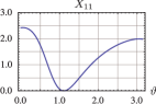
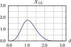
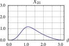
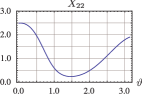
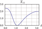
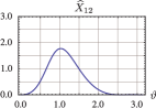
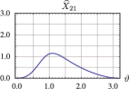
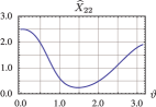
Figure 3: Matrix element squared for Compton scattering of polarized photons in the order $1\mapsto 1$, $1\mapsto 2$, $2\mapsto 1$, and $2\mapsto 2$ for each row. The functions in the first row correspond to Eq. (10.3), where the modified polarization vectors were plugged in. The panels in the second row show the corresponding function from Eq. (10.5) that is obtained by using polarization tensors instead of the polarization vectors directly. The plots were made for the special choice $\varphi=0$ and the horizontal axis gives the polar angle $\vartheta$. The Lorentz-violating parameters are chosen as $\widetilde{\kappa}^{01}=\widetilde{\kappa}^{02}=\widetilde{\kappa}^{03}=1/10$. Furthermore, $k_{1}=10^{-10}m$ and $m=1$.

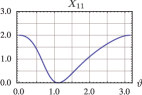
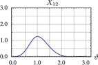
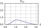
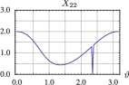
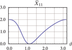
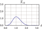
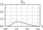
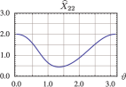
Figure 4: Same as Fig. 3, but now for the choice $\widetilde{\kappa}^{01}=\widetilde{\kappa}^{02}=\widetilde{\kappa}^{03}=10^{-10}$.

In Fig. 3, for which $\widetilde{\kappa}^{01}=\widetilde{\kappa}^{02}=\widetilde{\kappa}^{03}=1/10$ was inserted, we see that $X_{\lambda\lambda^{\prime}}$ corresponds to $\widehat{X}_{\lambda\lambda^{\prime}}$ for the processes $1\mapsto 1$, $1\mapsto 2$, $2\mapsto 1$, and $2\mapsto 2$. The graphs in Fig. 4 for Lorentz-violating parameters $\widetilde{\kappa}^{01}=\widetilde{\kappa}^{02}=\widetilde{\kappa}^{03}=10^{-10}$ indicate that for the $2\mapsto 2$ process the amplitude square $X_{\lambda\lambda^{\prime}}$ approaches $\widehat{X}_{\lambda\lambda^{\prime}}$, but there remains a residue, which appears for $X_{\lambda\lambda^{\prime}}$ as a narrow peak at an angle $\vartheta_{0}\approx 2.35$ (given in arc measure). Finally, in Fig. 5 we depict $X_{\lambda\lambda^{\prime}}$ and $\widehat{X}_{\lambda\lambda^{\prime}}$ for the $1\mapsto 1$ and the $2\mapsto 2$ modified Compton scattering as a function of both the polar angle $\vartheta$ and the azimuthal angle $\varphi$. It is evident that $X_{\lambda\lambda^{\prime}}$ and $\widehat{X}_{\lambda\lambda^{\prime}}$ for $1\mapsto 1$ perfectly agree with each other. This is also the case for the processes $1\mapsto 2$ and $2\mapsto 1$, but we will not display the corresponding plots here. However, the $2\mapsto 2$ scattering behaves differently. The matrix element $\widehat{X}_{\lambda\lambda^{\prime}}$ looks smooth, whereas for $\widetilde{\kappa}^{01}=\widetilde{\kappa}^{02}=\widetilde{\kappa}^{03}=1/10$, the amplitude square $X_{\lambda\lambda^{\prime}}$ is characterized by a set of sharp peaks. For small Lorentz violation some of these peaks seem to remain. Whether or not the limit for vanishing Lorentz violation is influenced by such structures cannot be investigated numerically, but requires analytical computations.

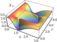
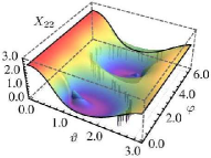
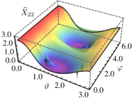
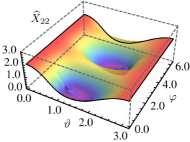
Figure 5: Matrix element squared dependent on the polar angle $\vartheta$ and the azimuthal angle $\varphi$ for Compton scattering of polarized photons. The plots in the first row were made by using $X_{\lambda\lambda^{\prime}}$ from Eq. (10.3). The graphs in the second row illustrate $\widehat{X}_{\lambda\lambda^{\prime}}$ from Eq. (10.5). The first column illustrates the corresponding functions for the $1\mapsto 1$ process with $\widetilde{\kappa}=1/10$. The second and the third demonstrate the $2\mapsto 2$ process, where $\widetilde{\kappa}=1/10$ and $\widetilde{\kappa}=10^{-10}$, respectively. Here again holds $k_{1}=10^{-10}m$ and $m=1$.

X.4 Interpretation

X.4.1 Discrepancies between $X_{\lambda\lambda^{\prime}}$ and $\widehat{X}_{\lambda\lambda^{\prime}}$ for $2\mapsto 2$ scattering

We already know from Eq. (5.2) that the second polarization vector splits into two contributions: a transverse and a longitudinal part. For vanishing Lorentz violation it is explicitly true that

$$(\varepsilon^{(2)\,\mu})=(\varepsilon^{0},\widehat{\boldsymbol{\varepsilon}}^{\,(2)}_{\mathrm{transv}}+\varepsilon^{0}\,\widehat{\mathbf{k}})=(0,\widehat{\boldsymbol{\varepsilon}}^{\,(2)}_{\mathrm{transv}})+\varepsilon^{0}\,(1,\widehat{\mathbf{k}})=(0,\widehat{\boldsymbol{\varepsilon}}^{\,(2)}_{\mathrm{transv}})+\frac{\varepsilon^{0}}{|\mathbf{k}|}\,(k^{\mu})\,,$$ (10.8a)

$$\widehat{\boldsymbol{\varepsilon}}^{\,(2)}_{\mathrm{transv}}=\widehat{\mathbf{k}}\times(\widehat{\mathbf{k}}\times\widehat{\boldsymbol{\zeta}})\,.$$ (10.8b)

If $\varepsilon^{(2)\,\mu}$ couples to a gauge-invariant quantity, its longitudinal part will vanish because of the Ward identity, since it is directly proportional to the four-momentum $k^{\mu}$.

The weird structures appearing in the matrix element squared $X_{22}$, which were discussed in the last section, originate from the longitudinal part of $\varepsilon^{(2)\,\mu}$. As mentioned, from Eq. (10.8) it follows that in the limit of zero Lorentz violation the longitudinal part vanishes by the Ward identity when contracted with physical quantities. However, this only holds if the prefactor $\varepsilon^{0}$ is not zero. Otherwise, we run into a “$0/0$” situation, which is mathematically not defined. Now, the physical phase space of the process contains a sector, for which $|k_{\parallel}|$ becomes arbitrarily small. This sector is characterized by two angles $(\varphi_{0},\vartheta_{0})$, where for $\varphi_{0}=0$, $\vartheta_{0}\approx 2.35$. This is depicted in Fig. 6.

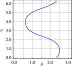
Figure 6: Contour of angles $(\varphi_{0},\vartheta_{0})$, for which the normalization factor $N^{\prime\prime}$ vanishes. The peaks in Fig. 5, lie on this contour.

For this special case the normalization factor $N^{\prime\prime}$ and, therefore, the prefactor $\varepsilon^{0}$ can become arbitrarily small. This destroys the applicability of the Ward identity and shows up as peaks in $X_{22}$ of Figs. 4 and 5.

Now we would like to analytically investigate the limit $\mathcal{E}\mapsto 0$ of the second polarization vector, with its transversal part subtracted. We distinguish between two cases, $k_{\parallel}\sim\mathcal{E}k_{\bot}$ and $k_{\parallel}\gg\mathcal{E}k_{\bot}$. The first represents the phase space sector for Compton scattering, for which $k_{\parallel}$ becomes arbitrarily small. We begin with the zeroth component of Eq. (5.3):

$$\sqrt{N^{\prime\prime}}\,\varepsilon^{0} =\frac{1}{4}\big{(}k^{2}-(k\cdot\xi)^{2}\big{)}\Big{(}(k\cdot\zeta)^{2}-\zeta^{2}\big{(}k^{2}-(k\cdot\xi)^{2}\big{)}\Big{)}$$

$$\sim\left\{\begin{array}[]{lcl}\mathcal{E}^{2}|\mathbf{k}|^{2}(k_{\parallel}^{2}+|\mathbf{k}|^{2})&\text{for}&k_{\parallel}\gg\mathcal{E}k_{\bot}\,,\\ \mathcal{E}^{2}k_{\bot}^{4}&\text{for}&k_{\parallel}\sim\mathcal{E}k_{\bot}\,.\\ \end{array}\right.$$ (10.11)

The longitudinal part $\boldsymbol{\varepsilon}_{\mathrm{long}}$, which can be extracted from Eq. (5.3) as well, results in:

$$\sqrt{N^{\prime\prime}}\,\boldsymbol{\varepsilon}_{\mathrm{long}}|^{\mathcal{E}\mapsto 0} \simeq\big{(}\sqrt{|\mathbf{k}|^{2}}+\mathbf{k}\cdot\boldsymbol{\zeta}\big{)}\big{(}\mathbf{k}\times(\mathbf{k}\times\boldsymbol{\zeta})\big{)}^{2}\frac{\mathbf{k}}{|\mathbf{k}|^{2}}$$

$$=\mathcal{E}^{2}|\mathbf{k}|^{4}\big{(}1+\mathcal{E}\widehat{\mathbf{k}}\cdot\widehat{\boldsymbol{\zeta}}\big{)}\big{(}\widehat{\boldsymbol{\zeta}}-\widehat{\mathbf{k}}(\widehat{\mathbf{k}}\cdot\widehat{\boldsymbol{\zeta}})\big{)}^{2}\,\widehat{\mathbf{k}}$$

$$=\mathcal{E}^{2}|\mathbf{k}|^{4}\big{(}1+\mathcal{E}\widehat{\mathbf{k}}\cdot\widehat{\boldsymbol{\zeta}}\big{)}\big{(}1-(\widehat{\mathbf{k}}\cdot\widehat{\boldsymbol{\zeta}})^{2}\big{)}\widehat{\mathbf{k}}$$

$$=\mathcal{E}^{2}|\mathbf{k}|^{4}\left(1+\frac{\mathcal{E}k_{\parallel}}{|\mathbf{k}|}\right)\left(1-\frac{k_{\parallel}^{2}}{|\mathbf{k}|^{2}}\right)\widehat{\mathbf{k}}$$

$$\sim\left\{\begin{array}[]{lcl}\mathcal{E}^{2}|\mathbf{k}|^{2}\big{(}|\mathbf{k}|^{2}-k_{\parallel}^{2}\big{)}\widehat{\mathbf{k}}&\text{for}&k_{\parallel}\gg\mathcal{E}k_{\bot}\,,\\ \mathcal{E}^{2}k_{\bot}^{4}\widehat{\mathbf{k}}&\text{for}&k_{\parallel}\sim\mathcal{E}k_{\bot}\,.\end{array}\right.$$ (10.14)

The normalization factor from Eq. (5.8) is

$$N^{\prime\prime}|^{\mathcal{E}\mapsto 0}\simeq\mathcal{E}^{2}k_{\bot}^{2}|\mathbf{k}|^{2}(4k_{\parallel}^{4}+4k_{\parallel}^{2}k_{\bot}^{2}+\mathcal{E}^{2}k_{\bot}^{2})\sim\left\{\begin{array}[]{lcl}4\mathcal{E}^{2}k_{\bot}^{2}k_{\parallel}^{2}|\mathbf{k}|^{4}&\text{for}&k_{\parallel}\gg\mathcal{E}k_{\bot}\,,\\ \mathcal{E}^{6}k_{\bot}^{8}&\text{for}&k_{\parallel}\sim\mathcal{E}k_{\bot}\,.\\ \end{array}\right.$$ (10.15)

Respecting $k_{\parallel}\gg\mathcal{E}k_{\bot}$, we obtain for the second polarization vector:

$$(\varepsilon^{(2)\,\mu}-\varepsilon^{(2)\,\mu}_{\mathrm{transv}})|^{k_{\parallel}\gg\mathcal{E}k_{\bot}} =\left.\frac{1}{\sqrt{N^{\prime\prime}}}\begin{pmatrix}\varepsilon^{0}\\ \boldsymbol{\varepsilon}_{\mathrm{long}}\\ \end{pmatrix}\right|^{k_{\parallel}\gg\mathcal{E}k_{\bot}}\sim\frac{\mathcal{E}^{2}|\mathbf{k}|^{2}}{\sqrt{4\mathcal{E}^{2}k_{\bot}^{2}k_{\parallel}^{2}|\mathbf{k}|^{4}}}\begin{pmatrix}k_{\parallel}^{2}+|\mathbf{k}|^{2}\\ \big{(}|\mathbf{k}|^{2}-k_{\parallel}^{2}\big{)}\widehat{\mathbf{k}}\\ \end{pmatrix}$$

$$=\frac{\mathcal{E}|\mathbf{k}|^{2}}{2k_{\bot}|k_{\parallel}||\mathbf{k}|^{2}}\begin{pmatrix}|\mathbf{k}|^{2}+k_{\parallel}^{2}\\ (|\mathbf{k}|^{2}-k_{\parallel}^{2})\widehat{\mathbf{k}}\\ \end{pmatrix}\,,$$ (10.16)

which vanishes for $\mathcal{E}\mapsto 0$. In contrast to the latter case, the result for $k_{\parallel}\sim\mathcal{E}k_{\bot}$ is as follows:

$$(\varepsilon^{(2)\,\mu}-\varepsilon^{(2)\,\mu}_{\mathrm{transv}})|^{k_{\parallel}\sim\mathcal{E}k_{\bot}} =\left.\frac{1}{\sqrt{N^{\prime\prime}}}\begin{pmatrix}\varepsilon^{0}\\ \boldsymbol{\varepsilon}_{\mathrm{long}}\\ \end{pmatrix}\right|^{k_{\parallel}\sim\mathcal{E}k_{\bot}}$$

$$\sim\frac{1}{\sqrt{\mathcal{E}^{6}k_{\bot}^{8}}}\begin{pmatrix}\mathcal{E}^{2}k_{\bot}^{4}\\ \mathcal{E}^{2}k_{\bot}^{4}\widehat{\mathbf{k}}\\ \end{pmatrix}=\frac{1}{\mathcal{E}}\begin{pmatrix}1\\ \widehat{\mathbf{k}}\\ \end{pmatrix}\,.$$ (10.17)

The latter diverges in the limit $\mathcal{E}\mapsto 0$.

Hence, it becomes evident that for vanishing Lorentz-violating parameter $\mathcal{E}$, when $k_{\parallel}$ runs into the phase space sector where it becomes of the order of $\mathcal{E}k_{\bot}$, a peak emerges. Its width is then $\sim\mathcal{E}k_{\bot}$ and its height is $\sim 1/\mathcal{E}$. This leads us undoubtedly to the following representation of a $\delta$-function as the limit of a function sequence:

$$\delta(x)=\lim_{n\mapsto 0}g_{n}(x)\,,\quad g_{n}(x)=\left\{\begin{array}[]{lcl}2/n&\text{for}&|x|\leq n\,,\\ 0&\text{for}&|x|>n\,.\\ \end{array}\right.$$ (10.18)

The role of the function sequence index $n$ in Eq. (10.18) is taken by the Lorentz-violating parameter $\mathcal{E}$ in the polarization vector. As a result, we finally obtain in the limit $\mathcal{E}\mapsto 0$:

$$(\varepsilon^{(2)\,\mu}-\varepsilon^{(2)\,\mu}_{\mathrm{transv}})|^{\mathcal{E}\mapsto 0}\sim k_{\bot}\delta(k_{\parallel})\begin{pmatrix}1\\ \widehat{\mathbf{k}}\\ \end{pmatrix}\,.$$ (10.19)

This analytic result shows, besides the numerically obtained plots in Figs. 4 and 5, that the longitudinal part of the second polarization vector may still play a role for vanishing Lorentz-violating parameter. Because of the $\delta$-function, the Ward identity can perhaps not be applied any more.

Now we want to look at the third term of Eq. (10.4), which is enclosed by round brackets. It will be denoted as $X^{(3)}_{\lambda\lambda^{\prime}}$ in what follows. We consider the $2\mapsto 2$ scattering process, where for the polarization vector in the final state we insert only its longitudinal part according to Eq. (10.19). Note that the longitudinal part of the initial state polarization vector vanishes, since $k_{1,\parallel}\neq 0$. Then we obtain:

$$X_{22}^{(3)} =\varepsilon^{(2)}(k_{1})\cdot\varepsilon^{(2)}(k_{2})-\frac{(\varepsilon^{(2)}(k_{1})\cdot p_{1})(\varepsilon^{(2)}(k_{2})\cdot p_{2})}{p_{1}\cdot k_{1}}+\frac{(\varepsilon^{(2)}(k_{1})\cdot p_{2})(\varepsilon^{(2)}(k_{2})\cdot p_{1})}{p_{1}\cdot k_{2}}$$

$$\sim k_{2,\bot}\delta(k_{2,\parallel})\begin{pmatrix}0\\ \widehat{\boldsymbol{\varepsilon}}^{(2)}(k_{1})\\ \end{pmatrix}\cdot\begin{pmatrix}1\\ \widehat{\mathbf{k}}_{2}\\ \end{pmatrix}$$

$$\quad\,-\frac{k_{2,\bot}\delta(k_{2,\parallel})}{p_{1}\cdot k_{1}}\left[\begin{pmatrix}0\\ \widehat{\boldsymbol{\varepsilon}}^{(2)}(k_{1})\\ \end{pmatrix}\cdot\begin{pmatrix}p_{1}^{0}\\ \mathbf{p}_{1}\\ \end{pmatrix}\right]\left[\begin{pmatrix}1\\ \widehat{\mathbf{k}}_{2}\\ \end{pmatrix}\cdot\begin{pmatrix}p_{2}^{0}\\ \mathbf{p}_{2}\\ \end{pmatrix}\right]$$

$$\quad\,+\frac{k_{2,\bot}\delta(k_{2,\parallel})}{p_{1}\cdot k_{2}}\left[\begin{pmatrix}0\\ \widehat{\boldsymbol{\varepsilon}}^{(2)}(k_{1})\\ \end{pmatrix}\cdot\begin{pmatrix}p_{2}^{0}\\ \mathbf{p}_{2}\\ \end{pmatrix}\right]\cdot\left[\begin{pmatrix}1\\ \widehat{\mathbf{k}}_{2}\\ \end{pmatrix}\cdot\begin{pmatrix}p_{1}^{0}\\ \mathbf{p}_{1}\\ \end{pmatrix}\right]$$

$$=k_{2,\bot}\delta(k_{2,\parallel})\left[\widehat{\boldsymbol{\varepsilon}}^{(2)}(k_{1})\cdot\widehat{k}_{2}-\frac{(\widehat{\boldsymbol{\varepsilon}}^{(2)}(k_{1})\cdot\mathbf{p}_{1})(p_{2}\cdot k_{2})}{|\mathbf{k}_{2}|\,p_{1}\cdot k_{1}}+\frac{(\widehat{\boldsymbol{\varepsilon}}^{(2)}(k_{1})\cdot\mathbf{p}_{2})(p_{1}\cdot k_{2})}{|\mathbf{k}_{2}|\,p_{1}\cdot k_{2}}\right]$$

$$=k_{2,\bot}\delta(k_{2,\parallel})\left[\widehat{\boldsymbol{\varepsilon}}^{(2)}(k_{1})\cdot\widehat{\mathbf{k}}_{2}-\frac{\widehat{\varepsilon}^{(2)}(k_{1})\cdot\mathbf{k}_{2}}{|\mathbf{k}_{2}|}\right]=0\,,$$ (10.20)

where we have used $\widehat{\boldsymbol{\varepsilon}}^{(2)}(k_{1})\cdot\mathbf{p}_{1}=0$. Hence, the Ward identity does not seem to care about the $\delta$-function. The contribution from the longitudinal part vanishes anyway. The conclusion is that the peaks in Fig. 5 are — most likely — numerical artifacts. Besides that, we expect this to hold also for the peaks in Fig. 4, where the Lorentz-violating parameter has the finite value $1/10$.

X.4.2 Limit of $\widehat{X}_{\lambda\lambda^{\prime}}$ for vanishing Lorentz violation

In section IX we have seen that preferred spacetime directions $\xi^{\mu}$ and $\zeta^{\mu}$ appear in the polarization tensors $\Pi_{\mu\nu}$ even for vanishing Lorentz violation. However, since the limit of $\widehat{X}_{\lambda\lambda^{\prime}}$ for vanishing Lorentz-violating parameters seems to coincide with the standard QED result, they obviously do not play a role for physical quantities. The question then arises as to why this is the case.

We consider an amplitude $\mathcal{M}$, to which one external photon with four-momentum $k^{\mu}$ and polarization $\lambda$ couples: $\mathcal{M}=\varepsilon_{\mu}^{(\lambda)}(k)\mathcal{M}^{\mu}(k)$. In what follows, the term “matrix element squared” is understood in the sense of individual contributions $|\varepsilon_{\mu}^{(\lambda)}(k)\mathcal{M}^{\mu}(k)|^{2}$. For a virtual state, all polarization vectors, hence also the scalar and the longitudinal ones, contribute to the polarization-summed matrix element squared — denoted as $|\mathcal{M}|^{2}$:

$$|\mathcal{M}|^{2}\Big{|}^{\mathrm{unphys}}\equiv\sum_{\lambda=0}^{3}|\varepsilon_{\mu}^{(\lambda)}(k)\mathcal{M}^{\mu}(k)|^{2}\,.$$ (10.21)

Evaluating $|\mathcal{M}|^{2}$ for a real state means that the Ward identity is used. For standard QED, if $(k^{\mu})=(k,0,0,k)$ is chosen, the Ward identity will result in

$$k^{\mu}\mathcal{M}_{\mu}=k_{0}\mathcal{M}_{0}-k_{3}\mathcal{M}_{3}=k(\mathcal{M}_{0}+\mathcal{M}_{3})=0\,,$$ (10.22)

from which it follows that $\mathcal{M}_{0}=-\mathcal{M}_{3}$ or $|\mathcal{M}_{0}|^{2}=|\mathcal{M}_{3}|^{2}$. Because of this, the unphysical degrees of freedom cancel each other and what remains are terms which involve the physical polarization vectors ($\lambda=1$, 2). Since the latter can be chosen as $(\varepsilon_{1}^{\mu})=(0,1,0,0)$ and $(\varepsilon_{2}^{\mu})=(0,0,1,0)$, we obtain

$$|\mathcal{M}|^{2}\Big{|}^{\mathrm{phys}}_{\mathrm{QED}}=\sum_{\lambda=1,2}|\varepsilon_{\mu}^{(\lambda)}(k)\mathcal{M}^{\mu}(k)|^{2}=|\mathcal{M}_{1}|^{2}+|\mathcal{M}_{2}|^{2}=\sum_{\lambda=1,2}|\mathcal{M}_{\lambda}|^{2}\,,$$ (10.23)

where ‘phys’ means that the Ward identity has been used.

In order to understand the limits of the polarization tensors from Eq. (9.3) we will perform a similar analysis in the context of the modified theory. For $(k^{\mu})=(|\mathbf{k}|,\mathbf{k})$ with $\mathbf{k}=(k_{\bot},0,k_{\parallel})$ the Ward identity reads

$$k^{\mu}\mathcal{M}_{\mu}=k_{0}\mathcal{M}_{0}-k_{1}\mathcal{M}_{1}-k_{3}\mathcal{M}_{3}=|\mathbf{k}|\mathcal{M}_{0}+k_{\bot}\mathcal{M}_{1}+k_{\parallel}\mathcal{M}_{3}=0\,,$$ (10.24)

and therefore, $\mathcal{M}_{1}$ can be expressed as follows:

$$\mathcal{M}_{1}=-\frac{|\mathbf{k}|}{k_{\bot}}\mathcal{M}_{0}-\frac{k_{\parallel}}{k_{\bot}}\mathcal{M}_{3}\,,$$ (10.25a)

$$|\mathcal{M}_{1}|^{2}=\frac{|\mathbf{k}|^{2}}{k_{\bot}^{2}}|\mathcal{M}_{0}|^{2}+\frac{k_{\scriptscriptstyle{\parallel}}^{2}}{k_{\bot}^{2}}|\mathcal{M}_{3}|^{2}+\frac{2|\mathbf{k}|k_{\parallel}}{k_{\bot}^{2}}\mathrm{Re}(\mathcal{M}_{0}\mathcal{M}_{3}^{*})\,.$$ (10.25b)

Using the result of Eq. (10.25b), the contribution of the matrix element squared involving the first polarization mode results in:

$$|\varepsilon_{\mu}^{(1)}\mathcal{M}^{\mu}|^{2}\Big{|}^{\mathrm{phys}}_{\begin{subarray}{c}\mathrm{mod}\\ \mathcal{E}\mapsto 0\end{subarray}} =|\mathcal{M}_{1}|^{2}+|\mathcal{M}_{2}|^{2}-\frac{1}{k_{\bot}^{2}}\left\{|\mathbf{k}|^{2}|\mathcal{M}_{0}|^{2}+k_{\scriptscriptstyle{\parallel}}^{2}|\mathcal{M}_{3}|^{2}+2|\mathbf{k}|k_{\parallel}\mathrm{Re}(\mathcal{M}_{0}\mathcal{M}_{3}^{*})\right\}\!\Big{|}^{\mathrm{phys}}$$

$$=\frac{1}{k_{\bot}^{2}}\left\{|\mathbf{k}|^{2}|\mathcal{M}_{0}|^{2}+k_{\scriptscriptstyle{\parallel}}^{2}|\mathcal{M}_{3}|^{2}+2|\mathbf{k}|k_{\parallel}\mathrm{Re}(\mathcal{M}_{0}\mathcal{M}_{3}^{*})\right\}+|\mathcal{M}_{2}|^{2}$$

$$\hskip 28.45274pt\,-\frac{1}{k_{\bot}^{2}}\left\{|\mathbf{k}|^{2}|\mathcal{M}_{0}|^{2}+k_{\scriptscriptstyle{\parallel}}^{2}|\mathcal{M}_{3}|^{2}+2|\mathbf{k}|k_{\parallel}\mathrm{Re}(\mathcal{M}_{0}\mathcal{M}_{3}^{*})\right\}$$

$$=|\mathcal{M}_{2}|^{2}\,,$$ (10.26)

where the Ward identity has been used in the second step. Hence, restricting the “matrix element squared” to the physical subspace with the Ward identity guarantees that the additional parts, that depend on the preferred directions $\xi^{\mu}$ and $\zeta^{\mu}$, cancel.

Now consider the $\lambda=2$ polarization mode. With Eq. (10.25b) we obtain:

$$|\varepsilon_{\mu}^{(2)}\mathcal{M}^{\mu}|^{2}\Big{|}^{\mathrm{phys}}_{\begin{subarray}{c}\mathrm{mod}\\ \mathcal{E}\mapsto 0\end{subarray}} =\frac{k_{\scriptscriptstyle{\parallel}}^{2}}{k_{\bot}^{2}}|\mathcal{M}_{0}|^{2}+\frac{|\mathbf{k}|^{2}}{k_{\bot}^{2}}|\mathcal{M}_{3}|^{2}+\frac{2|\mathbf{k}|k_{\parallel}}{k_{\bot}^{2}}\mathrm{Re}(\mathcal{M}_{0}\mathcal{M}_{3}^{*})\Big{|}^{\mathrm{phys}}$$

$$=\frac{k_{\scriptscriptstyle{\parallel}}^{2}}{k_{\bot}^{2}}|\mathcal{M}_{0}|^{2}+\frac{|\mathbf{k}|^{2}}{k_{\bot}^{2}}|\mathcal{M}_{3}|^{2}+\Bigl{\{}|\mathcal{M}_{1}|^{2}-\frac{|\mathbf{k}|^{2}}{k_{\bot}^{2}}|\mathcal{M}_{0}|^{2}-\frac{k_{\scriptscriptstyle{\parallel}}^{2}}{k_{\bot}^{2}}|\mathcal{M}_{3}|^{2}\Bigr{\}}$$

$$=\frac{k_{\scriptscriptstyle{\parallel}}^{2}-|\mathbf{k}|^{2}}{k_{\bot}^{2}}|\mathcal{M}_{0}|^{2}+|\mathcal{M}_{1}|^{2}+\frac{|\mathbf{k}|^{2}-k_{\scriptscriptstyle{\parallel}}^{2}}{k_{\bot}^{2}}|\mathcal{M}_{3}|^{2}$$

$$=-|\mathcal{M}_{0}|^{2}+|\mathcal{M}_{1}|^{2}+|\mathcal{M}_{3}|^{2}\,.$$ (10.27)

Setting $k_{\bot}=0$ in Eq. (10.24) results in $\mathcal{M}_{0}=-\mathrm{sgn}(k_{\parallel})\mathcal{M}_{3}$ and therefore $|\mathcal{M}_{0}|^{2}=|\mathcal{M}_{3}|^{2}$. This then leads to

$$|\varepsilon_{\mu}^{(2)}\mathcal{M}^{\mu}|^{2}\Big{|}^{\mathrm{phys}}_{\begin{subarray}{c}\mathrm{mod}\\ \mathcal{E}\mapsto 0\end{subarray}}=|\mathcal{M}_{1}|^{2}\,.$$ (10.28)

Hence, we see that by using the Ward identity all contributions depending on $\xi^{\mu}$ and $\zeta^{\mu}$ also vanish for the second mode. Therefore, for vanishing Lorentz violation the standard result

$$|\mathcal{M}|^{2}\Big{|}^{\mathrm{phys}}_{\begin{subarray}{c}\mathrm{mod}\\ \mathcal{E}\mapsto 0\end{subarray}}=\sum_{\lambda=1,2}|\varepsilon_{\mu}^{(\lambda)}\mathcal{M}^{\mu}|^{2}\Big{|}^{\mathrm{phys}}_{\begin{subarray}{c}\mathrm{mod}\\ \mathcal{E}\mapsto 0\end{subarray}}=|\mathcal{M}_{1}|^{2}+|\mathcal{M}_{2}|^{2}\,,$$ (10.29)

is recovered.

XI Discussion and conclusion

In this article, a special sector of a CPT-even Lorentz-violating modification of QED, with the characteristics of being parity-odd and nonbirefringent, was examined with respect to consistency. The deformation of QED is described by one fixed timelike “four-vector”, one fixed spacelike “four-vector”, and three Lorentz-violating parameters.

The nonbirefringent Ansatz combined with the parity-violating parameter choice leads to two distinct physical photon polarization modes. These modes are characterized by dispersion relations, that differ to quadratic order in the Lorentz-violating parameters. Hence, the theory is only nonbirefringent to linear order. The dispersion relations coincide with the formulas previously obtained in Ref. Casana-etal2009 . The new most important results of this article are summarized in the subsequent items:

• With the optical theorem, unitarity is verified for tree-level processes involving conserved currents.

• Microcausality is established for the full range of Lorentz-violating parameters. Information only propagates along the modified null cones.

• It has turned out that covariant polarization tensors can be constructed for each photon mode. This is not possible in standard QED, where only the polarization tensor of the sum of both modes can be written covariantly.

• The gauge-invariant polarization tensor of each mode depends on the background field directions. For vanishing Lorentz violation this dependence remains. It only cancels when considering the sum of both modes, which leads to the polarization sum of standard QED.

• The fact that the polarization tensors depend on the background field directions even for vanishing Lorentz violation, makes us think about the question of whether the limit of zero Lorentz violation is continuous. In other words, a priori it is not clear, whether or not the modified theory approaches standard QED for vanishing Lorentz violation. This is the motivation to test the theory via brute force by calculating one special process: Compton scattering for unpolarized electrons scattered by polarized photons.

• The cross sections can be computed either by using the modified polarization vectors or the modified polarization tensors. The upshot is that the results for $1\mapsto 1$, $1\mapsto~{}2$, and $2\mapsto 1$ coincide, but a numerical treatment reveals a discrepancy for $2\mapsto 2$ scattering. The Ward identity is shown to cure the polarization vectors and tensors from their bad behavior for vanishing Lorentz violation, at least for the first three processes. However, if the matrix element squared is computed for the fourth process by using the modified polarization vectors, there exists a phase space sector, for which the longitudinal part of the second polarization vector is proportional to a $\delta$-function. This could be shown by an analytic investigation. It could also be proven analytically that the Ward identity can cancel this contribution, nevertheless.

To conclude, the parity-odd “nonbirefringent” sector of modified Maxwell theory seems — with regard to the performed investigations — to be consistent. Further steps in the context of consistency of Lorentz-violating quantum field theories may involve the analysis of unitarity at one-loop level, where the Lorentz-violating structure is treated in an exact way. Especially for this parity-odd theory it would be interesting to know if its consistency is inherited to higher orders of perturbation theory. However, this is beyond the scope of this article.

In light of the consistency of this Lorentz-violating extension at tree level, nature decides on the values of the Lorentz-violating parameters. Therefore, they have to be measured with experiments. For a summary of the current experimental status we refer to Ref. Exirifard:2010xm and references therein. The latter article also gives new experimental bounds on the parity-odd parameters.

Appendix A Technical details concerning the calculation of the Compton cross sections

We compute the cross section in two different manners. The first possibility is to follow Sec. 11.1 of Ref. JauchRohrlich1976 , which gives the matrix element squared for Compton scattering of polarized photons off unpolarized electrons. In order to derive this equation, the authors use polarization vectors. This is clear since in standard QED covariant polarization tensors cannot be constructed from the polarization vectors. Hence, we perform a similar calculation in the modified theory, where we can directly test our polarization vectors given by Eqs. (5.1) and (5.2).

The second possibility is to compute the cross sections according to Eq. (5.81) of Ref. PeskinSchroeder1995 , where polarization tensors are used. Note that here Compton scattering of unpolarized photons is considered, hence it is averaged over initial and summed over final photon polarizations. Only under this condition can polarization tensors be used in standard QED. However, for parity-odd “nonbirefringent” modified Maxwell theory an analogous computation is also possible for Compton scattering with polarized photons. Hence, we have to calculate

$$\widetilde{\sigma}_{1X} =\frac{1}{4m\omega_{1}(\mathbf{k}_{1})|\mathbf{v}_{\mathrm{gr},\,1}|}\sum_{\lambda^{\prime}=1,2}\int\frac{\mathrm{d}^{3}k_{2}}{(2\pi)^{2}2\omega_{\lambda^{\prime}}(\mathbf{k}_{2})2E_{2}}\,\delta\big{(}\omega_{1}(\mathbf{k}_{1})+m-\omega_{\lambda^{\prime}}(\mathbf{k}_{2})-E_{2}\big{)}$$

$$\hskip 71.13188pt\,\times\big{(}|\mathcal{M}(k_{1},k_{2})|^{2}\big{)}^{\mu\nu\varrho\sigma}\big{(}\Pi_{\mu\varrho}(k_{1})|_{\lambda=1}\big{)}\big{(}\Pi_{\nu\sigma}(k_{2})|_{\lambda^{\prime}}\big{)}\Big{|}_{\begin{subarray}{c}k_{1}^{0}=\omega_{1}(\mathbf{k}_{1})\\ k_{2}^{0}=\omega_{\lambda^{\prime}}(\mathbf{k}_{2})\end{subarray}}\,,$$ (A.1a)

$$\widetilde{\sigma}_{2X} =\frac{1}{4m\omega_{2}(\mathbf{k}_{1})|\mathbf{v}_{\mathrm{gr},\,2}|}\sum_{\lambda^{\prime}=1,2}\int\frac{\mathrm{d}^{3}k_{2}}{(2\pi)^{2}2\omega_{\lambda^{\prime}}(\mathbf{k}_{2})2E_{2}}\,\delta\big{(}\omega_{2}(\mathbf{k}_{1})+m-\omega_{\lambda^{\prime}}(\mathbf{k}_{2})-E_{2}\big{)}$$

$$\hskip 71.13188pt\,\times\big{(}|\mathcal{M}(k_{1},k_{2})|^{2}\big{)}^{\mu\nu\varrho\sigma}\big{(}\Pi_{\mu\varrho}(k_{1})|_{\lambda=2}\big{)}\big{(}\Pi_{\nu\sigma}(k_{2})|_{\lambda^{\prime}}\big{)}\Big{|}_{\begin{subarray}{c}k_{1}^{0}=\omega_{2}(\mathbf{k}_{1})\\ k_{2}^{0}=\omega_{\lambda^{\prime}}(\mathbf{k}_{2})\end{subarray}}\,,$$ (A.1b)

where the energy of the final electron is denoted as $E_{2}$. Note the division by the group velocity of the first and second polarization state (see also Ref. Colladay:2001wk ), respectively, where in the standard theory $|\mathbf{v}_{\mathrm{gr},\,1}|=|\mathbf{v}_{\mathrm{gr},\,2}|=1$. The tensor $(|\mathcal{M}(k_{1},k_{2})|^{2}\big{)}^{\mu\nu\varrho\sigma}$ is given by the trace term of Eq. (5.81) of Ref. PeskinSchroeder1995 with some modifications due to the Lorentz-violating kinematics.

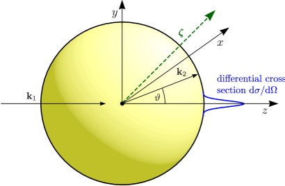
Figure 7: Chosen coordinate system for the phase space integration, where the initial photon three-momentum $\mathbf{k}_{1}$ lies along the third axis of the coordinate system. For the outgoing photon momentum $\mathbf{k}_{2}$, spherical coordinates are chosen with the azimuthal angle $\vartheta$ corresponding to the angle between $\mathbf{k}_{2}$ and the third axis. Cases are treated with the three-vector $\boldsymbol{\zeta}$ having equal or unequal components.

The purely algebraic part of the calculation, that includes computation of traces, contraction of indices and inserting kinematical relations, is performed with Form Vermaseren:2000nd . The subsequent phase space calculation is done numerically with C++, since the resulting matrix element squared contains hundreds of terms. The limit of zero Lorentz violation has to be taken with care and “long double” precision does not suffice here. Therefore, the GNU Multiple Precision Arithmetic Library GMP GMP:2011 is used with its C++ interface described in Sec. 12 of the reference previously mentioned.

The first idea was to choose the coordinate system such that $\boldsymbol{\zeta}$ lies along the third axis. Then the phase space should have been integrated with cylindrical coordinates $(k_{2,\bot},\varphi,k_{2,\parallel})$. To cover a general situation, where the initial photon momentum $\mathbf{k}_{1}$ points in an arbitrary direction, the cylindrical axes would have to point in that direction as well. As a result of this, the coordinate frame must be rotated in order to compute the cross section. This treatment has turned out to be unsuitable. Therefore, a better approach is the following, which is sketched in Fig. 7. The phase space integration is performed with spherical coordinates $(|\mathbf{k}_{2}|,\vartheta,\varphi)$, where the initial photon momentum points along the third axis of the coordinate system. The general case is mimicked by $\boldsymbol{\zeta}$ pointing in an arbitrary direction. As a special — but nevertheless very generic — case we can choose its components to be equal (however, computations were also done for different cases as shown in Table 5):

$$\boldsymbol{\zeta}=\widetilde{\kappa}\begin{pmatrix}1\\ 1\\ 1\\ \end{pmatrix}\,,\quad\mathcal{E}=\sqrt{3}\,|\widetilde{\kappa}|\,.$$ (A.2)

The integration over $|\mathbf{k}_{2}|$ is eliminated at once with the energy conservation equation in the $\delta$-function. Here, we have to keep in mind that

$$\delta \big{(}\omega_{\lambda}(k_{1})+m-\omega_{\lambda^{\prime}}(k_{2})-E_{2}\big{)}=$$

$$\hskip 56.9055pt\left|\frac{\partial\big{(}\omega_{\lambda}(k_{1})+m-\omega_{\lambda^{\prime}}(k_{2})-E_{2}\big{)}}{\partial k_{2}}\right|^{-1}\delta\big{(}k_{2}-(k_{2})^{0}\big{)}\,,\quad\lambda,\,\lambda^{\prime}\in\{1,2\}\,,$$ (A.3)

where $(k_{2})^{0}$ is the corresponding zero. The analytic solution $(k_{2})^{0}$ is a complicated function of $\mathcal{E}$ and $m$, so we determine it numerically with Newton’s method inside the C++ program. The integrations over $\vartheta$ and $\varphi$ are performed with the Simpson rule, which is sufficient for our purpose. The integration domain, that includes all physical states, is determined automatically with $(k_{2})^{0}$. If no zero $(k_{2})^{0}$ exists, then the corresponding angles $\vartheta$ and $\varphi$ lie outside the domain.

Appendix B Compton scattering and Thomson limit in standard (quantum) electrodynamics

The low-energy limit of the Compton scattering cross section (Thomson limit) can be calculated classically via the following equation (see e.g. Ref. Jackson:1975 ):

$$\left(\frac{\mathrm{d}\sigma}{\mathrm{d}\Omega}\right)^{\mathrm{Th}}_{\lambda\lambda^{\prime}}=\frac{\alpha^{2}}{m^{2}}|\overline{\boldsymbol{\varepsilon}_{f,\lambda^{\prime}}}\cdot\boldsymbol{\varepsilon}_{i,\lambda}|^{2}\,,$$ (B.1)

where $\boldsymbol{\varepsilon}_{i,\lambda}$ is the polarization three-vector of the incoming and $\boldsymbol{\varepsilon}_{f,\lambda^{\prime}}$ that of the outgoing electromagnetic wave. For the initial wave traveling along the $z$-axis we can choose the transverse polarization vectors as

$$\boldsymbol{\varepsilon}_{i,1}\equiv\begin{pmatrix}1\\ 0\\ 0\\ \end{pmatrix}\,,\quad\boldsymbol{\varepsilon}_{i,2}\equiv\begin{pmatrix}0\\ 1\\ 0\\ \end{pmatrix}\,.$$ (B.2)

In general, the propagation direction of the final wave can be described in spherical coordinates by the basis vector $\widehat{\mathbf{e}}_{r}=(\sin\vartheta\cos\varphi,\sin\vartheta\sin\varphi,\cos\vartheta)$. Then we can pick the physical polarization vectors to point along the other two basis vectors $\widehat{\mathbf{e}}_{\vartheta}$ and $\widehat{\mathbf{e}}_{\varphi}$:

$$\boldsymbol{\varepsilon}_{f,1}\equiv\widehat{\mathbf{e}}_{\vartheta}=\begin{pmatrix}\cos\vartheta\cos\varphi\\ \cos\vartheta\sin\varphi\\ -\sin\vartheta\\ \end{pmatrix}\,,\quad\boldsymbol{\varepsilon}_{f,2}\equiv\widehat{\mathbf{e}}_{\varphi}=\begin{pmatrix}-\sin\varphi\\ \cos\varphi\\ 0\\ \end{pmatrix}\,.$$ (B.3)

This leads to the polarized Thomson scattering cross sections in standard electrodynamics:

$$\sigma_{11}^{\mathrm{Th}}=\sigma_{21}^{\mathrm{Th}}=\frac{2\pi\alpha^{2}}{3m^{2}}\,,\quad\sigma_{12}^{\mathrm{Th}}=\sigma_{22}^{\mathrm{Th}}=\frac{2\pi\alpha^{2}}{m^{2}}\,.$$ (B.4)

If we rotate, for example, the set of initial polarization vectors by angle $\alpha$ and the final ones by angle $\beta$ in their corresponding polarization planes, the single contributions $\sigma_{\lambda\lambda^{\prime}}^{\mathrm{Th}}$ will depend on $\beta$. However, this dependence cancels in $\sigma_{1X}^{\mathrm{Th}}$ and $\sigma_{2X}^{\mathrm{Th}}$ that are defined as follows:

$$\sigma_{1X}^{\mathrm{Th}}\equiv\frac{1}{2}(\sigma_{11}^{\mathrm{Th}}+\sigma_{12}^{\mathrm{Th}})=\frac{4\pi\alpha^{2}}{3m^{2}}\,,$$ (B.5a)

$$\sigma_{2X}^{\mathrm{Th}}\equiv\frac{1}{2}(\sigma_{21}^{\mathrm{Th}}+\sigma_{22}^{\mathrm{Th}})=\frac{4\pi\alpha^{2}}{3m^{2}}\,,$$ (B.5b)

From $\sigma_{1X}^{\mathrm{Th}}=\sigma_{2X}^{\mathrm{Th}}$ is clear that both initial modes deliver equal contributions to the total Thomson result of Eq. (10.6).

This is also the case for MCS-theory. The MCS polarization tensors of Eq. (8.4) even give equal results for each individual polarized scattering process in the limit $m_{\mathrm{\scriptscriptstyle{CS}}}\mapsto 0$:

$$\sigma_{11}^{\mathrm{MCS,Th}}=\sigma_{12}^{\mathrm{MCS,Th}}=\sigma_{21}^{\mathrm{MCS,Th}}=\sigma_{22}^{\mathrm{MCS,Th}}=\frac{4\pi\alpha^{2}}{3m^{2}}\,,$$ (B.6)

For parity-odd modified “nonbirefringent” modified Maxwell theory the individual contributions are not equal for $\mathcal{E}\mapsto 0$. However, the above expressions from Eqs. (B.5a) and (B.5b) correspond to each other.

With Eq. (11-13) of Ref. JauchRohrlich1976 and the standard polarization vectors from Eq. (B.3) we obtain the polarized Compton scattering values given in Table. 2.

References

- (1) T. Adam et al. [OPERA Collaboration], “Measurement of the neutrino velocity with the OPERA detector in the CNGS beam,” arXiv:1109.4897 [hep-ex].
- (2) F. R. Klinkhamer, “Superluminal muon-neutrino velocity from a Fermi-point-splitting model of Lorentz violation,” arXiv:1109.5671 [hep-ph].
- (3) F. R. Klinkhamer and G. E. Volovik, “Superluminal neutrino and spontaneous breaking of Lorentz invariance,” Pisma Zh. Eksp. Teor. Fiz. 94, 731 (2011) [JETP Lett. 94 (2012) 673], arXiv:1109.6624 [hep-ph].
- (4) M. Schreck, “Multiple Lorentz groups — a toy model for superluminal muon neutrinos,” J. Mod. Phys. 3, 1398 (2012), arXiv:1111.7268 [hep-ph].
- (5) C. R. Contaldi, “The OPERA neutrino velocity result and the synchronisation of clocks,” arXiv:1109.6160 [hep-ph].
- (6) O. Besida, “Three errors in the article: ’The OPERA neutrino velocity result and the synchronisation of clocks’,” arXiv:1110.2909 [hep-ph].
- (7) R. A. J. van Elburg, “Measuring time of flight using satellite-based clocks,” arXiv:1110.2685 [physics.gen-ph].
- (8) C. S. Wu, E. Ambler, R. W. Hayward, D. D. Hoppes und R. P. Hudson, “Experimental test of parity conservation in beta decay” Phys. Rev. 105, 1413 (1957).
- (9) J. H. Christenson, J. W. Cronin, V. L. Fitch, R. Turlay, “Evidence for the decay of the meson,” Phys. Rev. Lett. 13, 138 (1964).
- (10) S. Chadha and H. B. Nielsen, “Lorentz invariance as a low-energy phenomenon,” Nucl. Phys. B 217, 125 (1983).
- (11) J. A. Wheeler, “On the nature of quantum geometrodynamics,” Annals Phys. 2, 604 (1957).
- (12) S. W. Hawking, “Space-time foam,” Nucl. Phys. B 144, 349 (1978).
- (13) D. Colladay and V. A. Kostelecký, “Lorentz-violating extension of the standard model,” Phys. Rev. D 58, 116002 (1998), arXiv:hep-ph/9809521.
- (14) V. A. Kostelecký and M. Mewes, “Electrodynamics with Lorentz-violating operators of arbitrary dimension,” Phys. Rev. D 80, 015020 (2009), arXiv:0905.0031 [hep-ph].
- (15) V. A. Kostelecký and M. Mewes, “Neutrinos with Lorentz-violating operators of arbitrary dimension,” Phys. Rev. D 85, 096005 (2012), arXiv:1112.6395 [hep-ph].
- (16) M. Cambiaso, R. Lehnert and R. Potting, “Massive photons and Lorentz violation,” Phys. Rev. D 85, 085023 (2012), arXiv:1201.3045 [hep-th].
- (17) P. Jordan and W. Pauli, “Zur Quantenelektrodynamik ladungsfreier Felder,” Z. Phys. 47, 151 (1928).
- (18) V. A. Kostelecký and R. Lehnert, “Stability, causality, and Lorentz and CPT violation,” Phys. Rev. D 63, 065008 (2001), arXiv:hep-th/0012060.
- (19) C. Adam and F. R. Klinkhamer, “Causality and CPT violation from an Abelian Chern–Simons-like term,” Nucl. Phys. B 607, 247 (2001), arXiv:hep-ph/0101087.
- (20) S. Liberati, S. Sonego and M. Visser, “Faster-than-c signals, special relativity, and causality,” Annals Phys. 298, 167 (2002), arXiv:gr-qc/0107091.
- (21) N. E. Mavromatos, “High-energy gamma-ray astronomy and string theory,” J. Phys. Conf. Ser. 174, 012016 (2009), arXiv:0903.0318 [astro-ph.HE].
- (22) R. Casana, M. M. Ferreira, A. R. Gomes, and P. R. D. Pinheiro, “Gauge propagator and physical consistency of the CPT-even part of the standard model extension,” Phys. Rev. D 80, 125040 (2009), arXiv:0909.0544 [hep-th].
- (23) R. Casana, M. M. Ferreira, A. R. Gomes, and F. E. P. dos Santos, “Feynman propagator for the nonbirefringent CPT-even electrodynamics of the standard model extension,” Phys. Rev. D 82, 125006 (2010), arXiv:1010.2776 [hep-th].
- (24) F. R. Klinkhamer, M. Schreck, “Consistency of isotropic modified Maxwell theory: Microcausality and unitarity,” Nucl. Phys. B 848, 90 (2011), arXiv:1011.4258 [hep-th].
- (25) F. R. Klinkhamer and M. Schreck, “Models for low-energy Lorentz violation in the photon sector: Addendum to ‘Consistency of isotropic modified Maxwell theory’,” Nucl. Phys. B 856, 666 (2012), arXiv:1110.4101 [hep-th].
- (26) E. F. Beall, “Measuring the gravitational interaction of elementary particles,” Phys. Rev. D 1, 961 (1970).
- (27) S. R. Coleman, S. L. Glashow, “Cosmic ray and neutrino tests of special relativity,” Phys. Lett. B 405, 249 (1997), hep-ph/9703240.
- (28) D. F. Phillips, M. A. Humphrey, E. M. Mattison, R. E. Stoner, R. F. C. Vessot, R. L. Walsworth, “Limit on Lorentz and CPT violation of the proton using a hydrogen maser,” Phys. Rev. D 63, 111101 (2001), physics/0008230.
- (29) D. Bear, R. E. Stoner, R. L. Walsworth, V. A. Kostelecký, C. D. Lane, “Limit on Lorentz and CPT violation of the neutron using a two species noble gas maser,” Phys. Rev. Lett. 85, 5038 (2000), physics/0007049.
- (30) S. M. Carroll, G. B. Field, and R. Jackiw, “Limits on a Lorentz- and parity-violating modification of electrodynamics,” Phys. Rev. D 41, 1231 (1990).
- (31) V. A. Kostelecký and M. Mewes, “Signals for Lorentz violation in electrodynamics,” Phys. Rev. D 66, 056005 (2002), arXiv:hep-ph/0205211.
- (32) V. A. Kostelecký, M. Mewes, “Cosmological constraints on Lorentz violation in electrodynamics,” Phys. Rev. Lett. 87, 251304 (2001), arXiv:hep-ph/0111026.
- (33) Q. G. Bailey and V. A. Kostelecký, “Lorentz-violating electrostatics and magnetostatics,” Phys. Rev. D 70, 076006 (2004), arXiv:hep-ph/0407252.
- (34) Y. Itin, “On light propagation in premetric electrodynamics. Covariant dispersion relation,” J. Phys. A 42, 475402 (2009), arXiv:0903.5520 [hep-th].
- (35) F. W. Hehl, Y. N. Obukhov, Foundations of Classical Electrodynamics: Charge, Flux, and Metric (Progress in Mathematical Physics), 1st ed. (Birkhäuser, Boston, 2003).
- (36) M. Gomes, J. R. Nascimento, A. Y. .Petrov and A. J. da Silva, “On the aether-like Lorentz-breaking actions,” Phys. Rev. D 81, 045018 (2010), arXiv:0911.3548 [hep-th].
- (37) F. R. Klinkhamer and M. Risse, “Addendum: Ultrahigh-energy cosmic-ray bounds on nonbirefringent modified Maxwell theory,” Phys. Rev. D 77, 117901 (2008), arXiv:0806.4351 [hep-ph].
- (38) V. A. Kostelecký, N. Russell, “Data Tables for Lorentz and CPT Violation,” Rev. Mod. Phys. 83, 11 (2011), arXiv:0801.0287 [hep-ph].
- (39) W. Heitler, The Quantum Theory of Radiation, 3rd ed. (Oxford University Press, London, 1954).
- (40) J. M. Jauch and F. Rohrlich, The Theory of Photons and Electrons, 2nd ed. (Springer, New York, USA, 1976).
- (41) M. J. G. Veltman, Diagrammatica: The path to Feynman rules (Cambridge University Press, Cambridge, England, 1994).
- (42) L. Brillouin, Wave Propagation and Group Velocity (Academic, New York, USA, 1960).
- (43) C. Itzykson and J. B. Zuber, Quantum Field Theory (McGraw-Hill, New York, USA, 1980).
- (44) M. E. Peskin and D. V. Schroeder, An Introduction to Quantum Field Theory (Addison–Wesley, Reading, USA, 1995).
- (45) C. Kaufhold and F. R. Klinkhamer, “Vacuum Cherenkov radiation and photon triple-splitting in a Lorentz-noninvariant extension of quantum electrodynamics,” Nucl. Phys. B 734, 1 (2006), arXiv:hep-th/0508074.
- (46) Korpuskeln und Strahlung in Materie II. Corpuscles and Radiation in Matter II, vol. 34, in Handbuch Der Physik. Encyclopedia of Physics, edited by S. Flügge (Springer, Berlin Göttingen Heidelberg, 1958).
- (47) J.-P. Bocquet, D. Moricciani, V. Bellini, M. Beretta, L. Casano, A. D’Angelo, R. Di Salvo, A. Fantini et al., “Limits on light-speed anisotropies from Compton scattering of high-energy electrons,” Phys. Rev. Lett. 104, 241601 (2010), arXiv:1005.5230 [hep-ex].
- (48) Q. Exirifard, “Cosmological birefringent constraints on light,” Phys. Lett. B 699, 1 (2011), arXiv:1010.2054 [gr-qc].
- (49) D. Colladay and V. A. Kostelecký, “Cross sections and Lorentz violation,” Phys. Lett. B 511, 209 (2001), hep-ph/0104300.
-
(50)
J. A. M. Vermaseren,
“New features of
FORM,” arXiv:math-ph/0010025. -
(51)
T. Granlund and the
GMPdevelopment team, “The GNU multiple precision arithmetic library, edition 5.0.2,”http://gmplib.org. - (52) J. D. Jackson, Classical Electrodynamics, 2nd ed., (John Wiley & Sons Inc, New York, USA, 1975).