The geometry of von-Neumann’s pre-measurement and weak values

Abstract

We have carried out a review of a paper from Tamate et al, conducting a deeper study of the geometric concepts they introduced in their paper, clarifying some of their results and calculations and advancing a step futher in their geometrization program for an understanding of the structure of von-Neumann’s pre-measurement and weak values.

I Introduction

The concept of a weak value of a quantum mechanical system was introduced in 1988 by Aharonov, Albert and Vaidman Aharonov et al. (1988). It was built on a time symmetrical model for quantum mechanics previously introduced by Aharonov, Bergmann and Lebowitz in 1964 Aharonov et al. (1964). In this model, non-local time boundary conditions are used, since the description of the state of a physical system between two quantum mechanical measurements is made by pre and post-selection of the states. The authors developed the so called ABL Rule for the transition probabilities within this scenario, so this is why it is also known as the two state formalism for quantum mechanics Aharonov and Vaidman (2007). The weak value of an observable can be considered as a generalization of the usual expectation value of a quantum observable, but differently from this, it takes values in the complex plane in general Jozsa (2007); Lobo and Ribeiro (2009a). The weak value concept has shown a plethora of theoretical and experimental applications. The issue of quantum counterfactuality, for instance, seems to be particularly less paradoxical when analyzed in terms of weak values Aharonov et al. (2002); Elitzur and Vaidman (1993). In quantum metrology, the amplification of tiny effects in quantum mechanics has spawn some recent impressive results as the observation of the spin Hall effect of light Hosten and Kwiat (2008). For a recent review on weak values, see Shikano (2011).

In our present work, we elaborate on a previous paper of Tamate et al where the authors introduce a very interesting geometric interpretation of the von Neumann pre-measurement and weak values which are closely related concepts. We conduct a review of their work, making the geometric structures more mathematically precise and advancing further in this geometrization programme. We also clarify some calculations and results from their original paper.

In the next section we review the von Neumann ideal pre-measurement formalism mostly to introduce our notation. In section III, we review Tamate et al’s geometric description of the interaction of a system with a discrete measuring system in a deeper mathematical manner based on the geometry of quantum mechanics developed by Berry and Aharonov-Anandan among many others dating back to the eighties Berry (1984); Aharonov and Anandan (1987). In section IV, we discuss their extension to infinite dimensional measuring systems with continuous indexed basis. We clarify the geometric content of a derivation of the intrinsic phase between two infinitesimally nearby states in the measured subsystem induced by an ideal von Neumann pre-measurement. The shift in position due to the instantaneous interaction with a measuring subsystem is shown to be proportional to the expectation value of the arbitrary observable $\hat{O}$ that is being measured in the first subsystem. We show how to conduct this derivation through a simple but deeper analysis of the geometrical structures involved. We also extend their calculation of the position shift in the measuring apparatus for initial states that results explicitly in a non-null imaginary part of the weak value. For the case of a single qubit this leads to a trivial geometric interpretation of this complex weak value. Finally, in section V, we address some concluding remarks and set stage for further work.

II The von Neumann pre-measurement model.

We discuss von Neumann’s model for a pre-measurement von Neumann (1996) where the measuring apparatus is also considered as a quantum system. Let $W=W_{S}\otimes W_{M}$ be the state vector space of the system formed by the subsystem $W_{S}$ and the measuring subsystem $W_{M}$. We will also assume that the measured system is a discrete quantum variable of $W_{S}$ defined by the observable $\hat{O}=|o_{i}\rangle o_{i}\langle o^{i}|$ (the sum convention will be used hereinafter). The measuring subsystem will be considered as a structureless (no spin or internal variables) quantum mechanical particle in one dimension. (In the next section we will consider discrete measuring systems.) Thus, we can choose as a basis for the vector state space $W_{M}$ either one of the usual eigenstates of position or momentum $\{|q(x)\rangle\}$ or $\{|p(x)\rangle\}$. It is important to note here that we use a slightly different notation than usual (for reasons that will soon become evident) in the sense that we distinguish between the “type” of the eigenvector ($q$ or $p$) from the actual $x$ eigenvalue Lobo and Ribeiro (2009a). For instance, we write:

$$\hat{Q}|q(x)\rangle=x|q(x)\rangle\qquad\text{and}\qquad\hat{P}|p(x)\rangle=x|p(x)\rangle.$$ (1)

(instead of $\hat{Q}|q\rangle=q|q\rangle$ and $\hat{P}|p\rangle=p|p\rangle$ as commonly written) where $\hat{Q}$ and $\hat{P}$ are the position and momentum observables subject to the well known Heisenberg relation: $[\hat{Q},\hat{P}]=i\hat{I}$ (hereinafter, $\hbar=1$ units will be used). With this non-standard notation, the completeness relation, normalization and the overlapping between these bases can be written respectively as:

$$\int\limits_{-\infty}^{+\infty}|q(x)\rangle\langle q(x)|dx=\int\limits_{-\infty}^{+\infty}|p(x)\rangle\langle p(x)|dx=\hat{I},$$

$$\langle q(x)|q(x\prime)\rangle=\langle p(x)|p(x\prime)\rangle=\delta(x-x\prime)$$ (2)

and

$$\langle q(x)|p(x\prime)\rangle=\dfrac{e^{ixx\prime}}{\sqrt{2\pi}}.$$ (3)

An ideal von-Neumann measurement can be defined as an instantaneous interaction between the two subsystems as modeled by the following delta-like time-pulse hamiltonian operator at time $t_{0}$:

$$\hat{H}_{int}(t)=\lambda\delta(t-t_{0})\hat{O}\otimes\hat{P},$$ (4)

where $\lambda$ is a parameter that represents the intensity of the interaction. This ideal situation models a setup where we are supposing that the time of interaction is very small compared to the time evolution given by the free Hamiltonians of both subsystems.

Let the initial state of the total system be given by the following unentangled product state: $|\psi_{i}\rangle=|\alpha\rangle\otimes|\varphi_{i}\rangle$ and the final state given by $|\psi_{f}\rangle=\hat{U}(t_{A},t_{B})|\psi_{i}\rangle\quad(t_{A}<t_{0}<t_{B})$, where the total unitary evolution operator is

$$\hat{U}(t_{A},t_{B})=e^{-i\int_{t_{A}}^{t_{B}}\hat{H}_{int}(t)dt}=e^{-i\lambda\hat{O}\otimes\hat{P}},$$ (5)

such that

$$(\hat{I}\otimes\langle q(x)|)|\psi_{f}\rangle=|o_{j}\rangle\otimes\langle q(x)|\hat{V}_{o_{j}}^{\dagger}|\varphi_{i}\rangle\alpha^{j},$$ (6)

where $|\alpha\rangle=|o_{j}\rangle\langle o^{j}|\alpha\rangle=|o_{j}\rangle\alpha^{j}$ and $\hat{V}_{\xi}$ is the one-parameter family of unitary operators in $W_{M}$ that implements the abelian group of translations in the position basis ($x,\xi\in\mathbb{R}$) as $\hat{V}_{\xi}|q(x)\rangle=|q(x-\xi)\rangle$. A correlation in the final state of the total system is then established between the variable to be measured $o_{j}$ with the continuous position variable of the measuring particle:

$$(\hat{I}\otimes\langle q(x)|)|\psi_{f}\rangle=|o_{j}\rangle\alpha^{j}\varphi_{i}(x-\lambda o_{j}),$$ (7)

where $\varphi_{i}(x)=\langle q(x)|\varphi_{i}\rangle$ is the wave-function in the position basis of the measuring system (the 1-D particle) in its initial state. This step of the von Neumann measurement prescription is called the pre-measurement of the system.

III A discrete measuring system

Let us consider now the measuring system as a finite dimensional quantum system $W_{M}^{(n)}$. In particular, if $n=2$, our measuring apparatus consists of a single qubit. We shall then start by initially treating this two-level measuring system so that we may make explicit use of Bloch sphere geometry and afterwards we shall extend this geometric treatment to infinite dimensional spaces.

III.1 Geometry of the space of rays.

Let $W^{n+1}$ be a $(n+1)$-dimensional Hilbert space together with its dual $\overline{W}^{n+1}$ and let also $\{|u_{\sigma}\rangle\}$ $(\sigma=0,1,...,n)$ be an arbitrary basis for $W^{n+1}.$ An hermitean inner product may be introduced by an ant-linear mapping ${\dagger}:W^{n+1}\longrightarrow\overline{W}^{n+1}$ (where ${\dagger}$ is the familiar “dagger” operation). Indeed, the inner product between two arbitrary states $|\psi\rangle$ and $|\varphi\rangle$ can now be defined as

$$(|\psi\rangle,|\varphi\rangle)=|\psi\rangle\left({}^{\dagger}|\varphi\rangle\right)=\langle\psi|\varphi\rangle.$$

Thus, an arbitrary normalized ket $|\psi\rangle$ expanded in such a basis can be represented by a complex $(n+1)$-column matrix:

$$|\psi\rangle=|u_{\sigma}\rangle\psi^{\sigma}\equiv\left(\psi_{0}\psi_{1}...\psi_{n}\right)^{\intercal},\quad\text{with\quad}\overline{\psi}_{\sigma}\psi^{\sigma}=1.$$ (8)

Writing the complex amplitudes as $\psi^{\sigma}=x^{\sigma}+iy^{\sigma}$ one can easily see that the set of normalized states can be identified with a $(2n+1)$-dimensional sphere $S^{2n+1}\subset\mathbb{C}^{n+1}$. Since two state vectors that differ by a complex phase cannot be physically distinguished by any means, it is convenient to define the true physical space of states as the above defined set of normalized states modulo the equivalence relation in $S^{2n+1}$ defined as

$$|\psi\rangle\sim|\varphi\rangle\iff\exists\quad\theta\in\mathbb{R}\ /\ |\psi\rangle=e^{i\theta}|\varphi\rangle.$$

The space of rays defined above is also known as the $n$-dimensional (complex) projective space $\mathbb{CP}(n)$. A standard complex coordinate system for $\mathbb{CP}(n)$ is provided by $n$ complex numbers $\xi^{i}=\psi^{i}\diagup\psi^{0}$ ($i=1,...,n$) for those points where $\psi^{0}\neq 0$. In the $n=1$ case we have a single qubit described by a single complex coordinate $\xi$. In this case, $\mathbb{CP}(1)$ is topologically equivalent to a $2D$ sphere and the stereographic projection map $\xi=\tan(\theta/2)e^{i\varphi}$ provides the Bloch sphere with standard coordinates. Thus, any physical state can be expressed as a normalized state represented as a point on the Bloch sphere in the following standard form

$$|\psi\rangle=|\theta,\varphi\rangle=\cos\left(\theta/2\right)|u_{0}\rangle+e^{i\varphi}\sin\left(\theta/2\right)|u_{1}\rangle,$$ (9)

where one can easily see that antipode points in the Bloch sphere represent orthogonal state vectors. In the concluding chapter, we shall see that the complex number $\xi=\tan(\theta/2)e^{i\varphi}$ can be directly physically measured as a certain appropriate weak value for two level systems.

III.2 The pre-measuring interaction

Suppose now that the interaction happens in $W=W_{S}\otimes W_{M}^{(m)}$ where the dimension of the measuring system is finite:

$$\dim W_{M}^{(m)}=m.$$

The initial separable pure-state is $|\psi_{(i)}\rangle=|\alpha\rangle\otimes|\varphi_{(i)}\rangle$ and $\{|v_{\sigma}\rangle\}$ $(\sigma=0,1,...,m-1)$ is the finite momentum basis of $W_{M}^{(m)}$ so the momentum observable can be expressed as $\hat{P}=|v_{\sigma}\rangle p_{\sigma}\langle v^{\sigma}|$. As in the first section, we model our instantaneous interaction with the hamiltonian $\hat{H}=\lambda\delta(t-t_{0})\hat{O}\otimes\hat{P}$, so that for $t_{f}>t_{0}>t_{i}$ one has:

$$|\psi_{(f)}\rangle=\hat{U}(t_{i},t_{f})|\psi_{(i)}\rangle=e^{-i\lambda p_{\sigma}\hat{O}}|\alpha\rangle\otimes|v_{\sigma}\rangle\varphi^{\sigma},$$ (10)

where we have expanded $|\varphi_{(i)}\rangle\in W_{M}^{(m)}$ in the finite momentum basis $\{|v_{\sigma}\rangle\}$. We can now define

$$|A_{\sigma}\rangle=e^{-i\lambda p_{\sigma}\hat{O}}|\alpha\rangle.$$ (11)

So that the final state of the overall system at $t_{f}$ will be:

$$|\psi_{(f)}\rangle=|A_{\sigma}\rangle\otimes|v_{\sigma}\rangle\varphi^{\sigma}.$$ (12)

The above entangled state clearly establishes a finite index correlation between $|A_{\sigma}\rangle$ $\in$ $W_{S}$ and the finite momentum basis $|v_{\sigma}\rangle$. The total system is in the pure state $|\psi_{(f)}\rangle\langle\psi_{(f)}|$ and by tracing out the first subsystem, the measuring system will be:

$$\hat{\rho}_{|\psi_{(f)}\rangle}^{(m)}=|v_{\sigma}\rangle\varphi^{\sigma}\langle A^{\tau}|A_{\sigma}\rangle\bar{\varphi}_{\tau}\langle v^{\tau}|.$$ (13)

Following Tamate et al, we consider the second subsystem (the measuring system) as a single qubit. In this case one may define

$$|\varphi_{(i)}\rangle=\cos(\theta/2)|v_{0}\rangle+\sin(\theta/2)e^{i\varphi}|v_{1}\rangle,$$

with

$$\langle A^{0}|A_{1}\rangle=|\langle A^{0}|A_{1}\rangle|e^{-i\beta},$$

so that we can compute the probability $p(\beta)$ of finding the second subsystem in a reference state $|\theta=\pi/2,\varphi=0\rangle$ as

$$\begin{split}p(\beta)&=tr\left(\hat{\rho}_{|\psi_{(f)}\rangle}^{(m)}|\pi/2,0\rangle\left\langle\pi/2,0\right|\right)\\ &=\frac{1}{2}+\frac{1}{4}|\langle A^{0}|A_{1}\rangle|\sin{\theta}\cos(\varphi-\beta).\end{split}$$ (14)

For a fixed angle $\theta$, this probability is maximized when $\varphi=\beta$. This fact can be used to measure the so called geometric phase $\beta=\arg(\langle A^{1}|A_{0}\rangle)$ between the two indexed states $|A_{0}\rangle$ and $|A_{1}\rangle$ $\in$ $W_{S}$. This definition of a geometric phase was originally proposed in 1956 by Pancharatnam Pancharatnam (1956) for optical states and rediscovered by Berry in 1984 Berry (1984) in his study of the adiabatic cyclic evolution of quantum states. In 1987, Anandan and Aharonov Aharonov and Anandan (1987) gave a description of this phase in terms of geometric structures of the $U(1)$ fiber-bundle structure over the space of rays and of the symplectic and Riemannian structures in the projective space $\mathbb{CP}(n)$ inherited from the hermitean structure of $W_{S}$.

III.3 Phase change due to post-selection

Given $|\psi_{(f)}\rangle$ resulting from the interaction between both subsystems we post-select a state $|\beta\rangle$ of $W_{S}$. This procedure induces a phase change as we shall see. The resulting state after post-selection is clearly

$$|\psi_{(f)}^{p}\rangle=C(|\beta\rangle\langle\beta|\otimes\hat{I})(|A_{\sigma}\rangle\otimes|v_{\sigma}\rangle\varphi^{\sigma}),$$ (15)

where $C$ is an unimportant normalization constant. Because of the post-selection, the system is in a non-entangled state so that the partial trace of $\hat{\rho}_{|\psi_{(f)}^{p}\rangle}=|\psi_{(f)}^{p}\rangle\langle\psi_{(f)}^{p}|$ over the first subsystem gives us

$$|\varphi_{(f)}\rangle=C\langle\beta|A_{\sigma}\rangle\varphi^{\sigma}|v_{\sigma}\rangle.$$ (16)

Making the following phase choices $\langle\beta|A_{0}\rangle=|\langle\beta|A_{0}\rangle|e^{i\beta_{0}}$ and $\langle\beta|A_{1}\rangle=|\langle\beta|A_{1}\rangle|e^{-i\beta_{1}}$, we can again compute the probability of finding the second subsystem in state $|\pi/2,0\rangle$:

$$\begin{split}p&=\frac{C^{2}}{2}[|\langle\beta|A_{0}\rangle|^{2}\cos^{2}(\theta/2)+|\langle\beta|A_{1}\rangle|^{2}\sin^{2}(\theta/2)+\\ &+\sin\theta|\langle\beta|A_{0}\rangle\langle\beta|A_{1}\rangle|\cos(\varphi_{p}-\beta_{0}-\beta_{1})]\end{split}$$

For a fixed angle $\theta$, the maximum probability occurs for $\varphi_{p}=\beta_{0}+\beta_{1}=\arg(\langle\beta|A_{0}\rangle\langle A^{1}|\beta\rangle)$. This implies that there is an overall phase change $\Theta$ given by

$$\Theta=\varphi_{p}-\varphi=\arg(\langle A^{1}|\beta\rangle\langle\beta|A_{0}\rangle\langle A^{0}|A_{1}\rangle).$$ (17)

The quantity given by (17) is a geometric invariant in the sense that it depends only on the projection of the state vectors $|A_{0}\rangle$, $|A_{1}\rangle$ and $|\beta\rangle$ on $\mathbb{CP}(n)$. In fact, this quantity is the intrinsic geometric phase picked by a state vector that is parallel transported through the closed geodesic triangle defined by the projection of the three states on ray space.

For a single qubit, the geometric invariant is proportional to the area of the geodesic triangle formed by the projection of the kets ($|A_{0}\rangle$, $|A_{1}\rangle$ and $|\beta\rangle$) on Bloch sphere and it is well known to be given by

$$\Theta=\arg(\langle A^{0}|\beta\rangle\langle\beta|A_{1}\rangle\langle A^{1}|A_{0}\rangle)=-\frac{\Omega}{2},$$ (18)

where $\Omega$ is the oriented solid angle formed by the geodesic triangle.

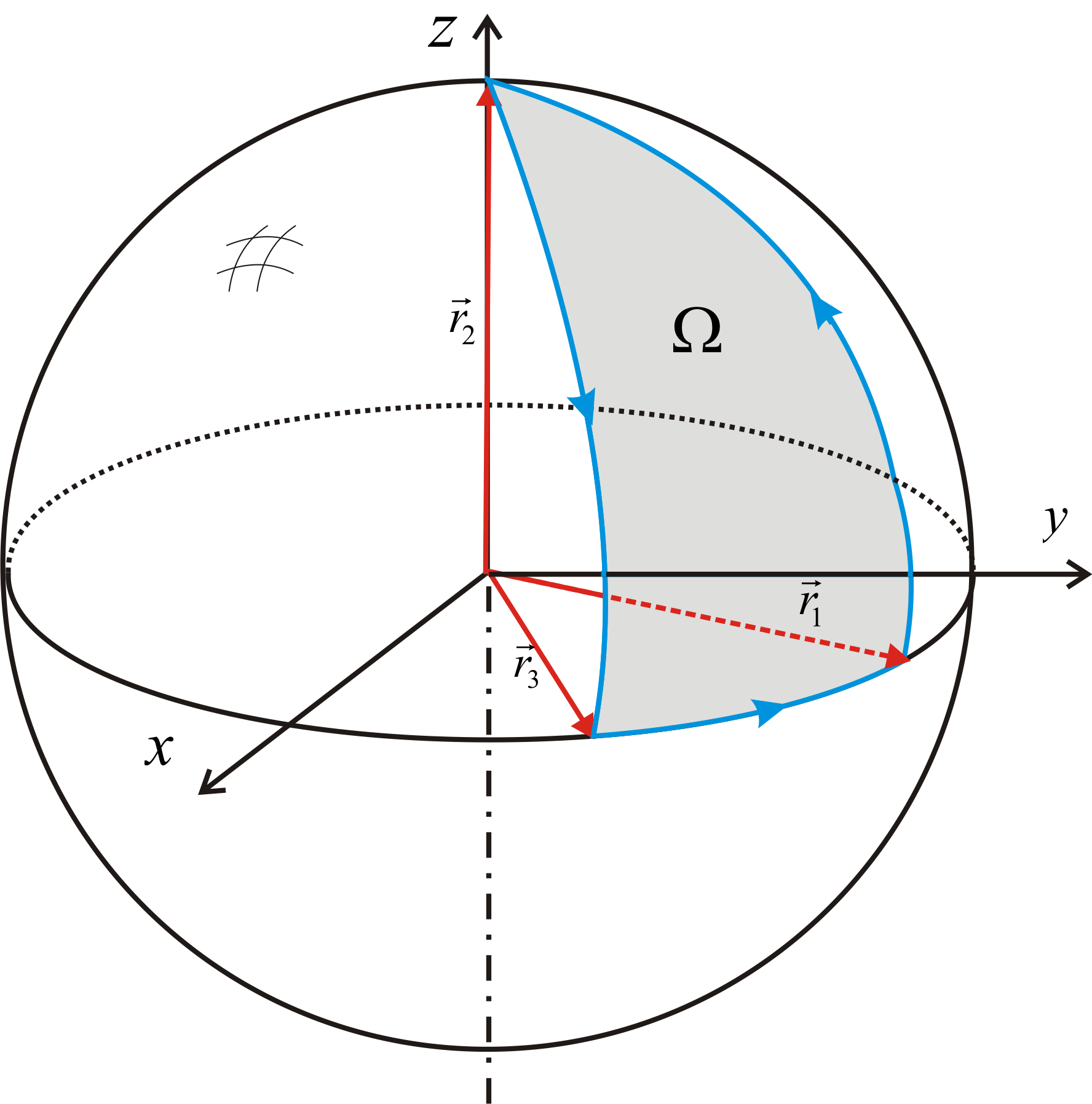
Figure 1: Solid angle determined by 3 points: the north pole and 2 points on the equator of the Bloch sphere.

IV The measuring system with a continuous base.

Suppose a physical system $W$ is composed by two subsystems $W_{S}\otimes W_{M}^{(\infty)}$ as before, but the measuring system $W_{M}^{(\infty)}$ is spanned  by complete sets of position kets $\{|q(x)\rangle\}$ (momentum kets $\{|p(y)\rangle\}$), with $-\infty<x,y<+\infty$. Let us consider $|\psi_{(i)}\rangle=|\alpha\rangle\otimes|\varphi_{(i)}\rangle$ as the initial product state and $\hat{H}=\lambda\delta(t-t_{0})\hat{O}\otimes\hat{P}$, with $\hat{P}=\int_{-\infty}^{+\infty}y|p(y)\rangle\langle p(y)|dy$, the hamiltonian that models the instantaneous measuring interaction so that the system evolves to

$$|\psi_{(f)}\rangle=\hat{U}(t_{i},t_{f})|\psi_{(i)}\rangle=\int_{-\infty}^{+\infty}dye^{-i\lambda y\hat{O}}|\alpha\rangle\otimes|p(y)\rangle\varphi_{p}(y),$$ (19)

where $\varphi_{p}(y)=\langle p(y)|\varphi_{(i)}\rangle$ is the momentum wave function associated to state $|\varphi_{(i)}\rangle$. We may define the state

$$|A(y)\rangle=e^{-i\lambda y\hat{O}}|\alpha\rangle,$$ (20)

so that we can rewrite the ket $|\psi_{(f)}\rangle$ as

$$|\psi_{(f)}\rangle=\int_{-\infty}^{+\infty}dy|A(y)\rangle\otimes|p(y)\rangle\varphi_{p}(y),$$ (21)

where the states $|A(y)\rangle$ are indexed by the continuous parameter $y\in\mathbb{R}$. We may now compute (to first order in $dy$) the intrinsic phase shift between $|A(y)\rangle$ and $|A(y+dy)\rangle$ in a similar way that was carried out in the previous section with the discretely parametrized states:

$$\arg(\langle A(y)|A(y+dy)\rangle)\approx-\lambda dy\langle\hat{O}\rangle_{|\alpha\rangle},$$ (22)

where $\langle\hat{O}\rangle_{|\alpha\rangle}=\langle\alpha|\hat{O}|\alpha\rangle$ is the expectation value of observable $\hat{O}$ in state $|\alpha\rangle$.

We can also compute the shift of the expectation value of the position observable $\hat{Q}$ of the particle of the measuring system between the initial and final states. Let $\{|o_{j}\rangle\},$ ($j=0,...,N-1$) be a complete set of eigenkets of observable $\hat{O}$. The final state of the composite system can be described by the following pure density matrix:

$$\hat{\rho}_{|\psi_{(f)}\rangle}=|\psi_{(f)}\rangle\langle\psi_{(f)}|=|o_{j}\rangle\langle o^{k}|\otimes\alpha^{j}\hat{V}_{\lambda o_{j}}^{\dagger}|\varphi_{(i)}\rangle\langle\varphi_{(i)}|\hat{V}_{\lambda o_{k}}\bar{\alpha}_{k}.$$ (23)

Taking the partial trace of the $W_{S}$ system, we arrive at the following mixed state that describes the measuring system at instant $t_{f}$:

$$\hat{\rho}_{|\psi_{(f)}\rangle}^{(M)}=\sum_{j}|\alpha^{j}|^{2}\hat{V}_{\lambda o_{j}}^{\dagger}|\varphi_{(i)}\rangle\langle\varphi_{(i)}|\hat{V}_{\lambda o_{j}}.$$ (24)

The ensemble expectation value $[\hat{Q}]_{\hat{\rho}_{|\psi_{(f)\rangle}}^{(M)}}$ of position is then given by:

$$[\hat{Q}]_{\hat{\rho}_{|\psi_{(f)}\rangle}^{(M)}}=tr(\hat{\rho}_{|\psi_{(f)}\rangle}^{(M)}\hat{Q})=\langle\hat{Q}\rangle_{|\varphi_{(i)}\rangle}+\lambda\langle\hat{O}\rangle_{|\alpha\rangle}.$$ (25)

The above result is similar to the one obtained by Tamate et al, yet we believe that the procedure we have adopted is mathematical more precise as we will discuss in the final concluding section of this paper. One may ask at this point if a similar procedure may be carried out in the case of weak values, since these can be thought of as a generalization of expectation values. The answer is affirmative, but before we demonstrate this, we shall discuss in the next section, a geometrical interpretation also inspired by Tamate et al’s description of the interaction between the system $W_{S}$ and the measuring system.

IV.1 Geometric interpretation of von Neumann’s pre-measurement

Let $W^{n+1}$ be a $(n+1)$-dimensional Hilbert space with basis $\{|u_{\sigma}\rangle\}$ so that an arbitrary (not necessarily normalized) vector of this space is described as $|\psi\rangle=|u_{\sigma}\rangle\psi^{\sigma}$, where greek indices take values in $\sigma=0,...,n$. One can map this state to a sphere $S^{2n+1}$ with radius given by

$$\bar{\psi}_{\sigma}\psi^{\sigma}=r^{2}.$$ (26)

We introduce projective coordinates $\xi^{i}$ on $\mathbb{CP}(n)$ so that

$$\psi^{0}=\frac{re^{i\varphi}}{(1+\bar{\xi}_{i}\xi^{i})^{1/2}},\quad\text{with}\quad i=1,...,n,$$ (27)

where $\varphi$ is an arbitrary phase factor. The euclidean metric in $W^{n+1}$, seen here as a $(2n+2)$-dimensional real vector space, can be written as Page (1987)

$$ds^{2}(W^{n+1})=d\psi^{\sigma}d\bar{\psi}_{\sigma}=dr^{2}+r^{2}ds^{2}(S^{2n+1}),$$ (28)

where

$$ds^{2}(S^{2n+1})=(d\varphi-A)^{2}+ds^{2}(\mathbb{CP}(n))$$ (29)

is the squared distance element over the space of normalized vectors, the $(2n+1)$-sphere, in $W^{n+1}$ and

$$A=\frac{i}{2}\left(\frac{\xi^{i}d\bar{\xi}_{i}-\bar{\xi}_{i}d{\xi}^{i}}{1+\bar{\xi}_{i}{\xi}^{i}}\right)$$ (30)

is the well known abelian 1-form connection of the $U(1)$ bundle over $\mathbb{CP}(n)$ and $ds^{2}$ is the metric over $\mathbb{CP}(n)$ in projective coordinates given explicitly by: Page (1987); Chruściński and Jamiołkowski (2004)

$$ds^{2}(\mathbb{CP}(n))=\left[\frac{(1+\bar{\xi}_{i}{\xi}^{i})\delta_{j}^{k}-\bar{\xi}_{k}\xi^{j}}{(1+\bar{\xi}_{i}{\xi}^{i})^{2}}\right]d\xi^{k}d\bar{\xi}_{j}.$$ (31)

A natural and intuitive picture of these structures can be seen easily in FIG. 2.

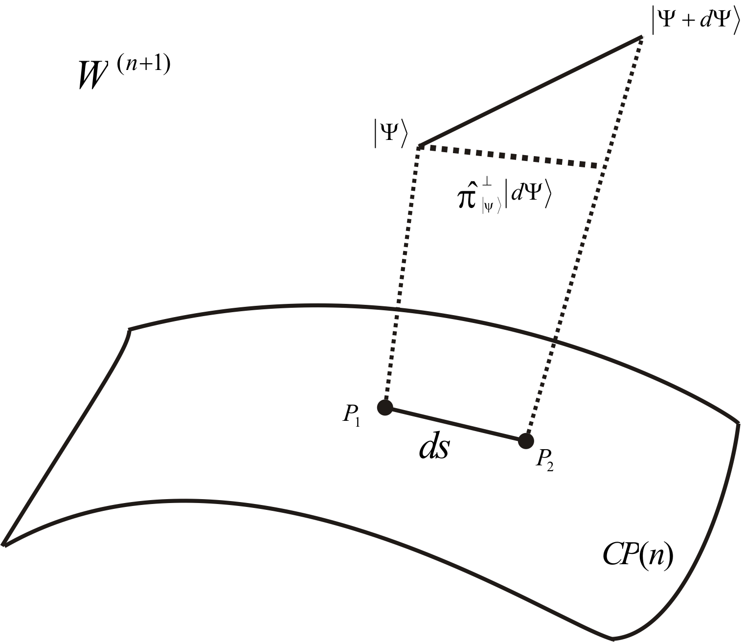
Figure 2: Pictorial representation of the quantum space of states

The points $P_{1}$ and $P_{2}$ $\in$ $\mathbb{CP}(n)$ are the projections respectively from two infinitesimally nearby normalized state vectors $|\psi\rangle$ and $|\psi+d\psi\rangle$. It is natural to define then, the squared distance between $P_{1}$ and $P_{2}$ as the projection of $|d\psi\rangle$ in the “orthogonal direction” of $|\psi\rangle$, that is, the projection given by the projection operator $\hat{\pi}_{|\psi\rangle}^{\perp}=\hat{I}-|\psi\rangle\langle\psi|$ as shown in 2. It is then easy to see that

$$ds^{2}(\mathbb{CP}(n))=\langle d\psi|d\psi\rangle-\langle d\psi|\psi\rangle\langle\psi|d\psi\rangle.$$ (32)

The above equation is an elegant manner to express (31). By inspecting both (29) and (32), it is not difficult to conclude that

$$(d\varphi-A)^{2}=\langle d\psi|\psi\rangle\langle\psi|d\psi\rangle.$$ (33)

Let $|\psi(t)\rangle$ be the curve of normalized state vectors in $W^{n+1}$ given by the unitary evolution generated by an hamiltonian $\hat{H}$. The Schrödinger equation implies a relation between $|\psi(t)\rangle$ and $|\psi(t+dt)\rangle$ given by:

$$|d\psi\rangle=|\psi(t+dt)\rangle-|\psi(t)\rangle=-i\hat{H}|\psi(t)\rangle dt.$$ (34)

The above equation together with (32) lead to a very elegant relation for the squared distance between two infinitesimally nearby projection of state vectors connected by the unitary evolution over $\mathbb{CP}(n)$ Anandan and Aharonov (1990):

$$\begin{split}ds^{2}(\mathbb{CP}(n))&=\left[\langle\psi(t)|\hat{H}^{2}|\psi(t)\rangle-(\langle\psi(t)|\hat{H}|\psi(t)\rangle)^{2}\right]dt^{2}\\ &=\left(\delta_{|\psi(t)\rangle}^{2}E\right)dt^{2}.\end{split}$$ (35)

One may say that the equation above means that the speed of the projection over $\mathbb{CP}(n)$ equals the instantaneous energy uncertainty

$$\frac{ds}{dt}=\delta E(t).$$ (36)

A beautiful geometric derivation of the time-energy uncertainty relation that follows directly from (36) can be found in Anandan and Aharonov (1990). Back to our discussion of the interaction between the systems $W_{S}$ and $W_{M}^{(\infty)}$, note that equation (20) is formally equivalent to the unitary time evolution equation $|\psi(t)\rangle=e^{-i\hat{H}t}|\psi(0)\rangle$ which is clearly a solution of a Schrödinger equation with time-independent hamiltonian. A formal analogy between the two distinct physical processes is exemplified by the association below:

$$\begin{array}[c]{ll}|\psi(t)\rangle&\mapsto|A(y)\rangle\\ |\psi(0)\rangle&\mapsto|\alpha\rangle=|A(0)\rangle\\ t&\mapsto y\\ \hat{H}&\mapsto\lambda\hat{O}.\end{array}$$

Looking at subsystem $W_{S}$ and regarding $y$ as an external parameter (just like the time variable for the unitary time evolution) we may write the analog of (35) in $\mathbb{CP}(n)\subset W_{S}$:

$$\begin{split}ds^{2}&=\left[\langle A(y)|\hat{O}^{2}|A(y)\rangle-\langle A(y)|\hat{O}|A(y)\rangle^{2}\right]\lambda^{2}dy^{2}\\ &=\left[\langle\alpha|\hat{O}^{2}|\alpha\rangle-\langle\alpha|\hat{O}|\alpha\rangle^{2}\right]\lambda^{2}dy^{2}.\end{split}$$ (37)

Comparing this result with (22) and (32), we advance one step further than Tamate et al in their geometrization programme as we present a geometric interpretation for the expectation value $\langle\alpha|\hat{O}|\alpha\rangle$ in terms of the $U(1)$ fiber bundle structure as one can easily infer from the pictorial representation in FIG. 3.

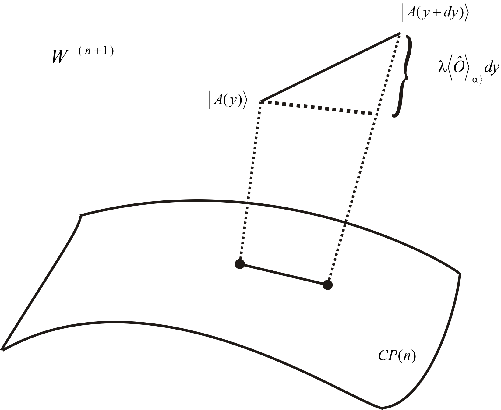
Figure 3: Pictorial representation of the phase difference between $|A(y)\rangle$ and $|A(y+dy)\rangle$.

IV.2 Post-selection and weak values

For the case of a weak measurement, the hamiltonian can be modeled as $\hat{H}^{(w)}=\epsilon\delta(t-t_{0})\hat{O}\otimes\hat{P}$, with $\epsilon\rightarrow 0$ Aharonov et al. (1988). Given the initial unentangled state $|\psi_{(i)}\rangle=|\alpha\rangle\otimes|\varphi_{(i)}\rangle$ at $t_{0}$, such that $t_{i}<t_{0}<t_{f}$, the system is described as

$$|\psi_{(f)}\rangle =\hat{U}(t_{i},t_{f})|\psi_{(i)}\rangle=e^{-i\epsilon\hat{O}\otimes\hat{P}}|\alpha\rangle\otimes|\varphi_{(i)}\rangle$$

$$=\int_{-\infty}^{+\infty}dy|A(y)\rangle\otimes|p(y)\rangle\varphi_{p}(y),$$

with $|A(y)\rangle=e^{-i\epsilon y\hat{O}}|\alpha\rangle$. The global geometric phase related to the infinitesimal geodesic triangle formed by the projections of $|A(y)\rangle$, $|A(y+dy)\rangle$ and the post-selected state $|\beta\rangle$ on $\mathbb{CP}(n)$ (see FIG. 4) is given by:

$$\Theta=\arg\left[\langle A(y)|\beta\rangle\langle\beta|A(y+dy)\rangle\langle A(y+dy)|A(y)\rangle\right].$$

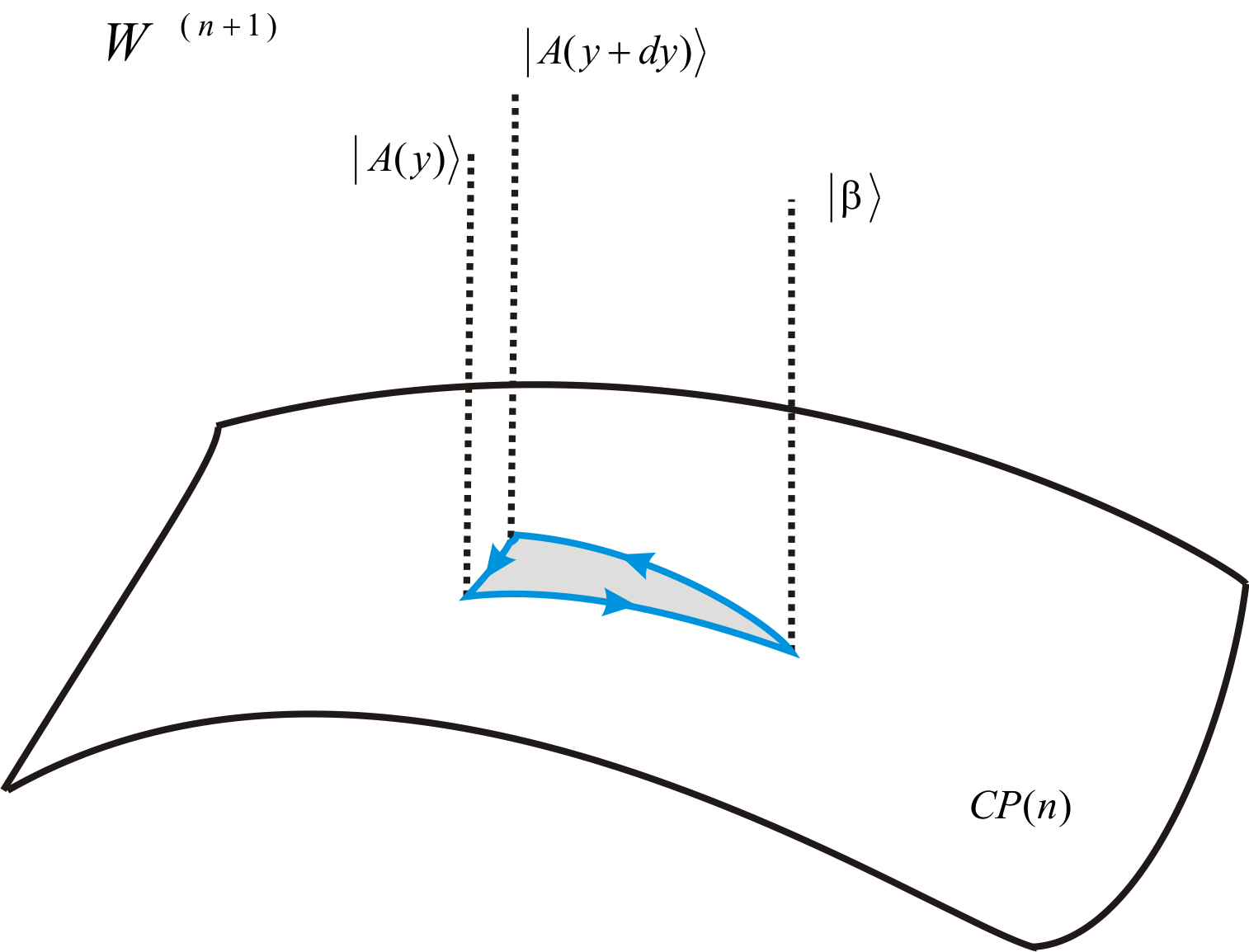
Figure 4: Pictorial representation of the global geometric phase.

Expanding to first order in $\epsilon$, we finally obtain

$$\Theta\approx-\epsilon\left[\operatorname{Re}({O}_{w})-\langle\hat{O}\rangle_{|\alpha\rangle}\right]dy,$$ (38)

where $O_{w}=\langle\beta|\hat{O}|\alpha\rangle/\langle\beta|\alpha\rangle$ is the weak value of $\hat{O}$ and $\langle\hat{O}\rangle_{|\alpha\rangle}$ is the expectation value of $\hat{O}$ in state $|\alpha\rangle$. Following the same approach of section III, we can compute the expectation value of the position observable $\hat{Q}$ of the measuring system $W_{M}^{(\infty)}$ between the initial and final states. The final state after post-selection of a state $|\beta\rangle$ of system $W_{S}$ is given by

$$|\psi_{(f)}\rangle =C(|\beta\rangle\langle\beta|\otimes\hat{I})(e^{-i\epsilon\hat{O}\otimes\hat{P}}|\alpha\rangle\otimes|\varphi_{(i)}\rangle)$$

$$\approx C(|\beta\rangle\langle\beta|\otimes\hat{I})(\hat{I}-i\epsilon\hat{O}\otimes\hat{P})|\alpha\rangle\otimes|\varphi_{\left(i\right)}\rangle,$$

where $C\approx(1+\epsilon\langle\hat{P}\rangle_{|\alpha\rangle}\operatorname{Im}({O}_{w}))\diagup\langle\beta|\alpha\rangle$ is the normalization constant because, in general, the state after post-selection is not normalized. By partial tracing out the first subsystem we arrive at:

$$\begin{split}\hat{\rho}_{|\psi_{(f)}\rangle}^{(2)}&=tr_{1}(|\psi_{(f)}\rangle\langle\psi_{(f)}|)\\ &=\left[1-i\epsilon\langle\hat{P}\rangle|\varphi_{\left(i\right)}\rangle({O}_{w}-\bar{O}_{w})\right]|\varphi_{\left(i\right)}\rangle\langle\varphi_{\left(i\right)}|-\\ &-i\epsilon({O}_{w}\hat{P}|\varphi_{\left(i\right)}\rangle\langle\varphi_{\left(i\right)}|-\bar{O}_{w}|\varphi_{\left(i\right)}\rangle\langle\varphi_{\left(i\right)}|\hat{P}),\end{split}$$

where $\langle\hat{P}\rangle_{|\varphi_{(i)}\rangle}$ is the expectation value of momentum $\hat{P}$ of the measuring system in state $|\varphi_{(i)}\rangle$ and $\bar{{O}}_{w}$ is the complex conjugate of the weak value ${O}_{w}$. The shift in the ensemble average $[\hat{Q}]_{\hat{\rho}_{|\psi_{(f)}\rangle}^{(2)}}=tr(\hat{\rho}_{|\psi_{(f)}\rangle}^{(2)}\hat{Q})$ can then be easily computed as $\Delta\hat{Q}=[\hat{Q}]_{\hat{\rho}_{|\psi_{(f)}\rangle}^{(2)}}-[\hat{Q}]_{\hat{\rho}_{|\psi_{(i)}\rangle}^{(2)}}$, giving us

$$\begin{split}\Delta\hat{Q}&=\epsilon\Big{[}(\operatorname{Im}(O_{w}))(\langle\varphi_{(i)}|\{\hat{Q},\hat{P}\}|\varphi_{(i)}\rangle-\\ &-2\langle\hat{P}\rangle_{|\varphi_{(i)}\rangle}\langle\hat{Q}\rangle_{|\varphi_{(i)}\rangle})+\operatorname{Re}(O_{w})\Big{]}.\end{split}$$ (39)

V Concluding Remarks

In Tamate et al. (2009), the authors introduced a very interesting geometric interpretation for von Neumann’s ideal pre-measurement concept as well as for the weak value. In this paper we have carried out a review of their paper, advancing a step further the geometric concepts they introduced in their paper and clarifying some of their results and calculations. For instance, the equation (22) below

$$\arg(\langle A(y)|A(y+dy)\rangle)\approx-\lambda dy\langle\hat{O}\rangle_{|\alpha\rangle}$$

is essentially the same result of equation 16 in Tamate et al. (2009):

$$\Theta(y)=\arg(\langle A(0)|A(y)\rangle)\approx-\lambda y\langle\hat{O}\rangle_{|\alpha\rangle}.$$ (40)

Yet, our approach seems to be more mathematically precise as it firmly grounded on the geometrical structures involved. The authors express a infinitesimal phase shift by differentiating a “function” $\Theta(y)$, but no such function exists because the geometric phase is obtained from the 1-form $A=i\left(\xi^{i}d\bar{\xi}_{i}-\bar{\xi}_{i}d{\xi}^{i}\right)\diagup 2\left(1+\bar{\xi}_{i}{\xi}^{i}\right)$. The exterior derivative $F=dA$ measures the local curvature of the connection form which measures the local lack of holonomy of the process of comparing intrinsic phases between normalized state vectors. This means that the 1-form $A$ is not the exterior derivative of any scalar function (a 0-form). The authors introduced this “function” $\Theta(y)$ and by formally taking its derivative, they managed to arrive at the correct equation

$$\Delta\hat{Q}=\lambda\langle\hat{O}\rangle.$$

This result is the same we obtained in (25), but, from the discussion above, it is quite clear that our approach seems to be mathematically more sound. The authors also approach a geometric interpretation of weak values, where they found the following equation for the shift in the expectation value of the position observable (equation 21 of Tamate et al. (2009)):

$$\Delta\hat{Q}=\epsilon\operatorname{Re}(O_{w}).$$

Yet it is well known that this result can be extended to a full complex-valued weak value (see Jozsa (2007) and Lobo and Ribeiro (2009b)). The above equation lacks a term proportional to the imaginary part of the weak value $O_{w}$ as one can see from equation (39). In fact, in their paper, they calculated an example for a qubit as the measuring system where they have chosen a very particular set of pre and post-selected states and observable that assures a weak value with null imaginary part. Indeed, if we choose the following: $\left|\alpha\right\rangle=\left|u_{0}\right\rangle$ (the “north pole” of the Bloch sphere), $\left|\beta\right\rangle=|\theta,\varphi\rangle=\cos\left(\theta/2\right)|u_{0}\rangle+e^{i\varphi}\sin\left(\theta/2\right)|u_{1}\rangle$ as respectively the pre and post-selected states and $\hat{O}=\hat{\sigma}_{1}=|u_{0}\rangle\left\langle u^{1}\right|+|u_{1}\rangle\left\langle u^{0}\right|$ as the observable, then it is straightforward to compute the weak value as $O_{w}=\tan\left(\theta/2\right)e^{i\varphi}$ which is clearly complex-valued in general. Yet, the post-selected $\left|\beta\right\rangle$ state chosen in Tamate et al. (2009) is equivalent to our choice with the phase $\varphi=0$. This is an arbitrary restriction over all possible choices of states in the Bloch sphere and only for $\varphi=0$ and $\varphi=\pi$ one arrives at a purely real weak value. What is curious about this result (for a single qubit) is that the weak value gives a direct physical meaning to the complex projective coordinate $\xi=\tan\left(\theta/2\right)e^{i\varphi}$. Indeed, when the experimentalist measures the (complete complex) weak value of a two level system in his lab, he actually is directly measuring the point on the $\mathbb{CP}(1)$ (complex plane + a point in infinity) of $\left|\beta\right\rangle$ related to the Bloch sphere by the stereographic projection. If the post-selected state is somewhere near the south pole, it is expected that there should be large measured distortions because of the nature of the projection. To remedy this, it is enough to rotate $\left|\alpha\right\rangle$ and $\hat{O}$ appropriately so that one can cover all states in $\mathbb{CP}(1)$ with good precision. It would be interesting to pursue further this kind of investigation of the geometrical meaning of weak values for higher dimensional systems. For instance, for higher spin systems, the geometry of spin coherent states could be useful for this purpose Perelomov (1986). In a preliminary version of our manuscript we have had the chance to see a reply of Tamate and collaborators to our paper. In their short reply they manage to explain further why they have restricted their attention only to the real part of the weak value. It became clear to us that the term

$$C(\hat{Q},\hat{P})=\langle\varphi_{(i)}|\{\hat{Q},\hat{P}\}|\varphi_{(i)}\rangle-2\langle\hat{P}\rangle_{|\varphi_{(i)}\rangle}\langle\hat{Q}\rangle_{|\varphi_{(i)}\rangle}$$

in equation (39) is expected to vanish for most experimental implementations. This is because for the usual initial states of the measuring apparatus, the position and momentum observables are uncorrelated. This is very unfortunate as our example shows that both imaginary and real parts of the weak value are true elements of reality that should be treated with the same ontological status. Maybe an experimental approach that focus on the geometric structures of the phase space of the measuring apparatus (the pointer) could furnish experimental methods to accomplish this as we have suggested in Lobo and Ribeiro (2009a).

The concept of weak values has lately become increasingly important both for theoretical and experimental reasons Popescu (2009). A deeper understanding of the physical and the mathematical structures behind weak values is of urgent need. One possible approach is to look at the phase space of the measuring system as was carried out in Lobo and Ribeiro (2009a). Another promising approach is the one initiated by Tamate et al in Tamate et al. (2009) where they look at the natural geometric structures of the measured system to characterize the weak value concept. We have tried to continue such geometrization programme by clarifying some conceptions in their original paper and advancing a step further in this approach. We introduced a geometric interpretation for the expectation value $\langle\hat{O}\rangle_{|\alpha\rangle}$ of an arbitrary observable $\hat{O}$ in terms of the $U(1)$ fiber bundle structure over the projective space of the measured subspace. We hope that this will lead to further fruitful theoretical and experimental applications. One possible research path is to consider the projective space structures of both subsystems and try to relate the exchange of information (in some kind of measure) between them in the (weak or strong) pre-measurement process in terms of these very same geometric structures.

References

- Aharonov et al. [1988] Y. Aharonov, D. Z. Albert, and L. Vaidman, Phys. Rev. Lett. 60, 1351 (1988).
- Aharonov et al. [1964] Y. Aharonov, P. G. Bergmann, and J. L. Lebowitz, Phys. Rev. 134, B1410 (1964).
- Aharonov and Vaidman [2007] Y. Aharonov and L. Vaidman, Time in Quantum Mechanics, Lecture Notes in Physics 734 (2007).
- Jozsa [2007] R. Jozsa, Phys. Rev. A 76, 044103 (pages 3) (2007), URL http://link.aps.org/abstract/PRA/v76/e044103.
- Lobo and Ribeiro [2009a] A. C. Lobo and C. A. Ribeiro, Phys. Rev. A 80, 012112 (2009a).
- Aharonov et al. [2002] Y. Aharonov, A. Botero, S. Popescu, B. Reznik, and J. Tollaksen, Physics Letters A 301, 130 (2002), ISSN 0375-9601, URL http://www.sciencedirect.com/science/article/pii/S03759601020%09866.
- Elitzur and Vaidman [1993] A. Elitzur and L. Vaidman, Foundations of Physics (Historical Archive) 23, 987 (1993).
- Hosten and Kwiat [2008] O. Hosten and P. Kwiat, Science 319, 787 (2008).
- Shikano [2011] Y. Shikano, Arxiv preprint arXiv:1110.5055 (2011).
- Berry [1984] M. Berry, Proceedings of the Royal Society of London. Series A, Mathematical and Physical Sciences 392, 45 (1984), ISSN 0080-4630.
- Aharonov and Anandan [1987] Y. Aharonov and J. Anandan, Physical Review Letters 58, 1593 (1987), ISSN 1079-7114.
- von Neumann [1996] J. von Neumann, Mathematical Foundations of Quantum Mechanics (Princeton University Press, 1996), ISBN 0691028931, URL http://www.amazon.ca/exec/obidos/redirect?tag=citeulike09-20%&path=ASIN/0691028931.
- Pancharatnam [1956] S. Pancharatnam, Proc. Indian Acad. Sci. A 44, 247 (1956).
- Page [1987] D. Page, Physical Review A 36, 3479 (1987), ISSN 1094-1622.
- Chruściński and Jamiołkowski [2004] D. Chruściński and A. Jamiołkowski, Geometric phases in classical and quantum mechanics (Birkhauser, 2004), ISBN 081764282X.
- Anandan and Aharonov [1990] J. Anandan and Y. Aharonov, Phys. Rev. Lett. 65, 1697 (1990), URL http://link.aps.org/doi/10.1103/PhysRevLett.65.1697.
- Tamate et al. [2009] S. Tamate, H. Kobayashi, T. Nakanishi, K. Sugiyama, and M. Kitano, New Journal of Physics 11, 093025 (2009).
- Lobo and Ribeiro [2009b] A. C. Lobo and C. A. Ribeiro, Phys. Rev. A 80, 012112 (2009b).
- Perelomov [1986] A. Perelomov, Generalized coherent states and their applications (Springer-Verlag New York Inc., New York, NY, 1986).
- Popescu [2009] S. Popescu, Physics 2, 32 (2009).