Bell Function Values Approach to Topological Quantum Phase Transitions

Abstract

We investigate the relation between Bell function values (BFV) of the reduced density matrix and the topological quantum phase transitions in the Kitaev-Castelnovo-Chamon model. We find that the first order derivative of BFV exhibits singular behavior at the critical point and we propose that it can serve as a good and convenient marker for the transition point. More interestingly, the value of the critical point can be analytically obtained in this approach. Since the BFV serves as a measure of nonlocality when it is greater than the classical bound of the correlation functions, our work has established a link between quantum nonlocality and phase transitions.

Topological phase of some strongly correlated quantum many body systems is a new kind of order that depends on the system topology Wen-Book . It has attracted great interest recently because it can exhibit remarkable phenomena such as quasiparticles with anyonic statistics. An archetypal physical realization of such phase is in the quantum Hall system 1990Prange-Book , which bears many unconventional characteristics, such as fractional statistical behaviors and ground state topological degeneracy that cannot be lifted by any local perturbations 1985Haldane . A particular interest in topological ordered states is their robustness against local perturbations which can lead to several consequences such as topological insulators 2009Hsieh and topological quantum computations 2008Nayak .

Not surprisingly, the unconventional properties of topological phase might result in exotic critical phenomena, which cannot be characterized by the Landau-Ginzburg-Wilson spontaneous symmetry-breaking theory where the correlation function of local order parameters plays a crucial role 1999Sachdev-Book . For example, the quantum phase transition between an Abelian and a non-Abelian topological phase in chiral spin liquid might be characterized by global flux and generalized topological entanglement entropy 2009Chung . More remarkably, for time-reversal invariant anyonic quantum systems, Gils et al., have recently showed that the topological phases could be uniformly described in terms of fluctuations of the two-dimensional surfaces and their topological changes 2009Gils . However, an universal characterization and detection of topological phase and its transitions still pose a big challenge despite a vast amount of prominent works dealing with this problem.

During the past few years, several important concepts in the quantum information field have been borrowed to characterize quantum phase transitions (QPTs) and topological quantum phase transitions (TQPTs), these including entanglement 2002Osterloh-entanglement , fidelity 2006Quan-Fidelity , fidelity susceptibility 2007You-FS , and discord 2008Dillenschneider-discord , etc. A brief review of the progress related to this issue is given in Ref. 2008Gu and references therein. Notwithstanding the great successes in marking QPTs and TQPTs in some physical systems, each approach above has its own disadvantages 2008Gu . Take the fidelity approach for example, to witness the QPTs, one has to find out the exact ground state. However, for most of the physical systems, finding out the exact ground state is very difficult. In addition, it is also a challenge to measure the fidelity in experiment on scalable systems. An alternative choice is to use Bell function values (BFV) as defined in expression (2) below, which indicates the correlations of a quantum system and measures quantum nonlocality when it is greater than the classical bound of the correlation functions 2009Forster . Actually, besides entanglement, quantum nonlcoality is also a central nonintuitive phenomena of quantum mechanics and it plays a key role in many quantum information and computation processes, such as quantum key distribution (KQD) 1991Ekert-Cryptograph , nonlocal quantum computation 2007Linden , etc. Naturely, one would ask whether nonlocality can mark QPTs and TQPTs?

In this Letter, we propose the use of BFV as the marker of TQPTs and provide a positive answer to the above question by investigating the relation between BFV of the reduced density matrix and the TQPTs. The motivation for choosing BFV is two-fold: (i) BFV can measure the nonlocality of a quantum system, thus it might establish a connection between nonlocality and TQPTs, which belong to two different aspects; (ii) To get the BFV in an experiment scheme, one only has to do some measurement on the qubits instead of knowing exactly the ground state. Thus, our approach has its advantages in experimental schemes. The discussion here is mainly based on the Kitaev-Castelnovo-Chamon model 2008Castelnovo , which exhibits a second-order TQPT at the critical point. Our results indicate that the first order derivative of BFV shows singular behavior at the transition point. More interestingly, through this approach, one can analytically obtain the critical value of the transition point. Finally, using BFV to signal TQPTs and QPTs in other systems is also briefly discussed.

Bell function values (BFV).—The famous Bell- Clauser-Horne-Shimony-Holt (Bell-CHSH) inequality for two entangled spin-$1/2$ (or qubit) particles, which has always provided an excellent test-bed for experimental verification of quantum mechanics against the predictions of local realism, is given by the inequality 1964Bell :

$$\mathcal{I}=Q_{11}+Q_{12}+Q_{21}-Q_{22}\leq 2,$$ (1)

where $Q_{ij}=\int_{\Gamma}\mu(\lambda)X_{1}(\mathbf{n}_{i}^{X_{1}},\lambda)X_{2}(\mathbf{n}_{j}^{X_{2}},\lambda)d\lambda$ is the correlation function with $X_{k}(\mathbf{n}_{m}^{X_{k}},\lambda)$ denoting the $m$-th observable on the $k$-th particle (here $i,j,k,m=1,2$); $\Gamma$ is the total space of the hidden variable $\lambda$ and $\mu(\lambda)$ is a statistical distribution of $\lambda$, satisfying $\int_{\Gamma}\mu(\lambda)d\lambda=1$. Quantum mechanically, the above inequality is violated by all pure entangled states of two qubits 1991Gisin-theory and the expression of the correlation function for any two-qubit state $\rho$ reads: $Q_{ij}^{Q}=\texttt{Tr}[(\mathbf{n}_{i}^{X_{1}}\cdot\vec{\sigma})\otimes(\mathbf{n}_{j}^{X_{2}}\cdot\vec{\sigma})\rho]$. Here $\mathbf{n}_{m}^{X_{k}}$ ($m,k=1,2$) are the unit vectors in three-dimensional Hilbert space and $\vec{\sigma}$ is the Pauli matrix vector. Based on the Bell-CHSH inequality (1), the Bell function values is defined as:

$$\mathscr{B}(\rho)\equiv\max\mathcal{I}^{Q},$$ (2)

where $\mathcal{I}^{Q}=Q_{11}^{Q}+Q_{12}^{Q}+Q_{21}^{Q}-Q_{22}^{Q}$ and the maximization is performed over all possible vectors $\mathbf{n}_{m}^{X_{k}}$. Generally speaking, for every specific two-qubit quantum state $\rho$, we need to carry out the procedure of the maximization to obtain its BFV $\mathscr{B}(\rho)$. Fortunately, in Ref. 1995Horodecki , the authors introduced another method to calculate $\mathscr{B}(\rho)$, which can circumvent the tedious maximization. It was proved there that

$$\mathscr{B}(\rho)=2\sqrt{\upsilon_{1}+\upsilon_{2}},$$ (3)

where $\upsilon_{1}$ and $\upsilon_{2}$ are the two greater eigenvalues of the $3\times 3$ symmetric matrix $\mathscr{L}_{\rho}^{\texttt{T}}\mathscr{L}_{\rho}$; $\mathscr{L}_{\rho}$ is a $3\times 3$ matrix with elements defined by $(\mathscr{L}_{\rho})_{\varsigma\tau}=\texttt{Tr}[\rho\sigma_{\varsigma}\otimes\sigma_{\tau}]$ ($\varsigma,\tau=1,2,3$) and $\mathscr{L}_{\rho}^{\texttt{T}}$ is the transpose of $\mathscr{L}_{\rho}$. In the experimental situation, in order to obtain the BFV, the observers of the first (second) qubit should carry out two measurements $\mathbf{n}_{1}^{X_{1}}\cdot\vec{\sigma}$ and $\mathbf{n}_{2}^{X_{1}}\cdot\vec{\sigma}$ ($\mathbf{n}_{1}^{X_{2}}\cdot\vec{\sigma}$ and $\mathbf{n}_{2}^{X_{2}}\cdot\vec{\sigma}$), just the same as in many Bell-CHSH inequality testing experiments 1982Aspect .

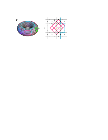
Figure 1: (Color online) An illustration of the Kitaev-Castelnovo-Chamon spin-lattice model and its map to the $2$D Ising model: In the KCC model, each black dot on the edge of the lattice represents a qubit and $\mathcal{V}$ and $\mathcal{F}$ denote the vertex and the face, respectively; The blue line across the lattices stands for a string operator along the non-trivial loop on the torus $\texttt{T}^{2}$. The system is invariant under transformation along the blue line 2009Chen . In its corresponding $2$D Ising model, the qubits live on the vertex (green dots). Mapping: $\sigma_{i}^{z}=\theta_{r}\theta_{r^{\prime}}$, where $i$ is the bond between the neighboring vertices $\langle r,r^{\prime}\rangle$. Thus, for $i$ and $j$ nearest neighbors, the mapping gives $\langle\sigma_{i}^{z}\sigma_{j}^{z}\rangle=\langle\theta_{r}\theta_{r^{\prime}}\theta_{r^{\prime\prime}}\theta_{r}\rangle=\langle\theta_{r^{\prime}}\theta_{r^{\prime\prime}}\rangle$, namely, the nearest qubits in KCC model become next-nearest in the corresponding $2$D Ising model.

The Kitaev-Castelnovo-Chamon (KCC) Model.—The physical model we consider in this article was introduced by Castelnovo and Chamon 2008Castelnovo , which is a deformation of the Kitaev toric code model 2003Kitaev . The Hamiltonian of the KCC model with periodic boundary conditions reads:

$$\mathscr{H}=-\mathcal{J}_{m}\sum_{\mathcal{F}\in\texttt{T}^{2}}B_{\mathcal{F}}-\mathcal{J}_{e}\sum_{\mathcal{V}\in\texttt{T}^{2}}A_{\mathcal{V}}+\mathcal{J}_{e}\sum_{\mathcal{V}\in\texttt{T}^{2}}e^{-\beta\sum_{j\in\mathcal{V}}\sigma^{z}_{j}},$$

where $\mathcal{J}_{m},\mathcal{J}_{e}>0$, $\beta$ is a coupling constant; $A_{\mathcal{V}}=\prod_{j\in\mathcal{V}}\sigma_{j}^{x}$ and $B_{\mathcal{F}}=\prod_{j\in\mathcal{F}}\sigma_{j}^{z}$ are the vertex and face operators in the original Kitaev toric code model 2003Kitaev . A brief sketch of this model is shown in Fig. 1. The ground state in the topological sector containing the fully magnetized state $|0\rangle=|\uparrow\uparrow\cdots\uparrow\rangle$ can be analytically obtained 2008Castelnovo :

$$|G(\beta)\rangle=\mathcal{Z}(\beta)^{-\frac{1}{2}}\sum_{g\in\mathcal{G}}e^{\beta\sum_{j}\sigma_{j}^{z}(g)/2}g|0\rangle,$$ (4)

where $\mathcal{Z}(\beta)=\sum_{g\in\mathcal{G}}e^{\beta\sum_{j}\sigma_{j}^{z}(g)}$; $\mathcal{G}$ is the Abelian group generated by the vertex operators $\{A_{\mathcal{V}}\}$ and $\sigma_{j}^{z}(g)$ is the value of spin at site $j$ in state $g|0\rangle$. Obviously, when $\beta=0$, $|G(\beta)\rangle$ reduces to the topologically ordered ground state of the toric code model 2003Kitaev , while when $\beta\rightarrow\infty$, $|G(\beta)\rangle$ becomes the fully magnetized state $|0\rangle$. At the point $\beta_{c}=\frac{1}{2}\ln(\sqrt{2}+1)$ there exists a second-order TQPT where the topological entanglement entropy $\mathcal{S}_{topo}=1$ for $\beta<\beta_{c}$ changes to $\mathcal{S}_{topo}=0$ for $\beta>\beta_{c}$ 2008Castelnovo .

As shown by Castelnovo and Chamon, there exists a one-to-two mapping between the configurations $\{g\}=\mathcal{G}$ the configurations $\{\theta\}$ of the classical $2$D Ising model 2008Castelnovo . In the mapping, the Hamiltonian of the Ising model has the form $\mathscr{H}_{Ising}=-\mathscr{C}\sum_{\langle r,r^{\prime}\rangle}\theta_{r}\theta_{r^{\prime}}$, where $\mathscr{C}$ is a coupling constant and $\theta_{r},\theta_{r^{\prime}}=+1$ or $-1$ depending on whether or not the corresponding vertex operator $A_{\mathcal{V}}$ is acting on the site $r$. Thus $\sigma^{z}_{i}=\theta_{r}\theta_{r^{\prime}}$ with $i$ being the edge between the nearest neighboring vertexes. An illustration of this mapping is shown in Fig. 1.

Signaling TQPTs by BFV.—Since the BFV introduced in expression (2) only account for two-qubit states, we need to calculate the reduced density matrix of two qubit $\rho_{ij}$ based on the ground state $|G(\beta)\rangle$ and the symmetry of the Hamiltonian $\mathscr{H}$. It was shown in Ref. 2009Eriksson that $\rho_{ij}$ has the following form (details are given in Ref. 2009Chen ; 2008Castelnovo and references there in):

$$\rho_{ij}=\frac{1}{4}[\mathbf{I}+\langle\sigma_{i}^{z}\rangle(\sigma^{z}_{i}+\sigma^{z}_{j})+\langle\sigma_{i}^{z}\sigma_{j}^{z}\rangle\sigma_{i}^{z}\sigma^{z}_{j}],$$ (5)

where $\mathbf{I}$ is the $4\times 4$ identity matrix. Based on the Eq. (5), the BFV can be calculated by using the simplified formula for $\mathscr{B}(\rho_{ij})$ in Eq. (3). For convenience and simplicity, we only concentrate on two cases where $i$ and $j$ are nearest and next-to-nearest neighbors, respectively. In the thermodynamic limit, the mapping to the $2$D Ising model gives that $\langle\sigma^{z}_{i}\rangle=\langle\theta_{r}\theta_{r^{\prime}}\rangle=-\coth(2\beta)[\pi+(4\tanh^{2}(2\beta)-2)\mathscr{X}(\chi)]/(2\pi)$, where $\mathscr{X}(\chi)=\int_{0}^{\pi/2}d\varphi(1-\chi^{2}\sin^{2}\varphi)^{-1/2}$ and $\chi=2\sinh(2\beta)/\cosh^{2}(2\beta)$. For the calculation of $\langle\sigma_{i}^{z}\sigma_{j}^{z}\rangle$, the equivalence between the $2$D Ising model and the quantum $1$D XY model yields:

(i) For $i$ and $j$ the nearest case, $\langle\sigma_{i}^{z}\sigma_{j}^{z}\rangle=\langle\theta_{r}\theta_{r^{\prime}}\rangle=\frac{1}{\pi}\int_{0}^{\pi}d\phi\{[\sinh^{-2}(2\beta)-\cos{\phi}]\cos{\phi}-\sin^{2}{\phi}\}/\{\sin^{2}{\phi}+[\sinh^{-2}(2\beta)-\cos{\phi}]^{2}\}^{1/2}$. Summarizing all the relations above enables us to obtain the BFV $\mathscr{B}(\rho_{ij})$. For the $i$ and $j$ nearest case, the numerical results for the first order derivative of BFV $\frac{d\mathscr{B}(\rho_{ij})}{d\beta}$ are displayed in Fig. 2(a), from which we see a distinct rapid increase of $\frac{d\mathscr{B}(\rho_{ij})}{d\beta}$ around the critical point $\beta_{c}\approx 0.44$. Note that we only focus on a small neighboring region of $\beta$ around the TQPT point $\beta_{c}$, namely $0.4\leq\beta\leq 0.5$. The smaller the $\delta\beta$, the greater the rapid increase. When $\delta\beta\rightarrow 0$, $\frac{d\mathscr{B}(\rho_{ij})}{d\beta}\rightarrow+\infty$, indicating its singularity at the TQPT point $\beta_{c}$.

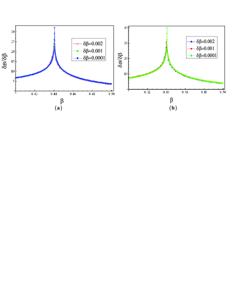
Figure 2: (Color online) Numerical results of the first order derivative of BFV $\mathscr{B}(\rho_{ij})$ versus $\beta$ for different $\delta\beta$. (a) $i$ and $j$ are the nearest case; (b) $i$ and $j$ are the next-to-nearest case.

More interestingly, after long tedious but straightforward calculations, we arrive at an analytical formula for $\frac{d\mathscr{B}(\rho_{ij})}{d\beta}$, which can enable us to obtain the analytical value of $\beta_{c}$:

$$\frac{d\mathscr{B}}{d\beta}=\int_{0}^{\pi}d\phi\texttt{csch}^{2}(2\beta)\sin^{2}\phi\Upsilon(\phi,\beta)/\pi,$$ (6)

Here $\Upsilon(\phi,\beta)=8\coth{(2\beta)}\texttt{csch}^{2}(2\beta)/(1-2\cos\phi\texttt{csch}^{2}(2\beta)+\texttt{csch}^{4}(2\beta))^{3/2}$. What is interesting is that we can analytically obtain the critical point from the Eq. (6). To this end, one can rewrite $\Upsilon(\phi,\beta)$ as $\Upsilon(\phi,\beta)=2\sqrt{2}\coth(2\beta)/\{[\frac{1}{2}(\texttt{csch}^{2}(2\beta)+1/\texttt{csch}^{2}(2\beta))-\cos\phi]^{3/2}\texttt{csch}(2\beta)\}$. Obviously, Eq. (6) has only one singular point because $\texttt{csch}^{2}(2\beta)+1/\texttt{csch}^{2}(2\beta)\geq 2$ and so the singularity happens at $\texttt{csch}^{2}(2\beta)+1/\texttt{csch}^{2}(2\beta)=2$, namely $\beta_{c}=\frac{1}{2}\ln(\sqrt{2}+1)$. This explicitly exhibits one of the advantages of BFV approach to TQPTs.

For $i$ and $j$ the next-to-nearest case, direct calculations show that $\langle\sigma_{i}^{z}\sigma_{j}^{z}\rangle=\cosh^{2}(\beta^{*})(\mathcal{T}_{-1}^{2}-\mathcal{T}_{-2}\mathcal{T}_{0})-\sinh^{2}(\beta^{*})(\mathcal{T}_{1}^{2}-\mathcal{T}_{2}\mathcal{T}_{0})$, where $\mathcal{T}_{\kappa}=\frac{1}{\pi}\int_{0}^{\pi}d\phi[(\xi-\cos{\phi})\cos{\kappa\phi}+\gamma\sin{\phi}\sin{\kappa\phi}]/[(\gamma\sin{\phi})^{2}+(\xi-\cos{\phi})^{2}]^{1/2}$. Here $\tanh(\beta^{*})=e^{-2\beta}$, $\gamma=[\cosh(2\beta^{*})]^{-1}$ and $\xi=(1-\gamma^{2})^{1/2}/\tanh(2\beta)$. We also plot the numerical results of $\frac{d\mathscr{B}(\rho_{ij})}{d\beta}$ in Fig. 2(b). From this figure, one can observe that the $\frac{d\mathscr{B}(\rho_{ij})}{d\beta}$ has a singularity at the TQPT point $\beta_{c}$. It is also obvious that $\frac{d\mathscr{B}(\rho_{ij})}{d\beta}$ behaves quite similarly between the nearest and next-to-nearest case. This result accords with the results in Ref. 2009Eriksson , where the reduced fidelity and reduced fidelity susceptibilities are only slightly different between the two cases, respectively. Since BFV indicates the qubit correlations in the system, it seems that the correlations of nearest qubits is similar as that of next-to-nearest qubits in topological ordered states. This is, to some extent, counterintuitive because in many physical systems the interaction between nearest particles is usually greater than that of next nearest particles.

It is worthwhile to note that the reduced density matrix $\rho_{ij}$ is diagonal. That indicates the correlations between any two local spins in the ground state of KCC model are always classical. Consequently, the Bell function values of $\rho_{ij}$ cannot be greater than $2$, the classical bound. Another interesting consideration here is similar to Ref. 2009Chen : we can calculate the BFV between a local qubit denoted by $i$ and the rest of the whole lattice by rewriting the ground state as $|\texttt{G}(\beta)\rangle=\mathscr{Y}_{+}|\mathscr{P}\rangle|0\rangle_{i}+\mathscr{Y}_{-}|\mathscr{Q}\rangle|1\rangle_{i}$, where $\mathscr{Y}^{2}_{\pm}=(1\pm\langle\theta_{0,0}\theta_{0,1}\rangle)/2$, $|\mathscr{P}\rangle$ and $|\mathscr{Q}\rangle$ are two orthogonal normalized vectors. Consequently, we can regard $|\texttt{G}(\beta)\rangle$ as a simple pure two-qubit entangled state. In this case, the BFV has a one-to-one monotonous relation with entanglement 1992Popescu , thus also with quantum discord since for pure two-qubit state, the quantum discord is the same as entanglement of entropy 2003Vedral . As a result, the BFV should behave similarly as the quantum discord does at the critical point $\beta_{c}$ (for details, see Ref. 2009Chen ). However, it is worthwhile to clarify that there is a distinctive difference between the BFV approach and the quantum discord approach. For the quantum discord, its value becomes trivially $0$ for the reduced two-qubit state, thus cannot signal the TQPT at the critical point. Nevertheless, as shown in the former paragraphs, the first order derivative of BFV is an excellent marker of the transitions. In addition, the physical meanings of BFV and quantum discord are different. Generally speaking, quantum discord is a measurement of the ‘quantumness’ of a system. While, BFV measures the nonlocality of the system when it is greater than the classical bound. In this case, $\mathscr{B}(|\texttt{G}(\beta)\rangle)=2\sqrt{1+4\mathscr{Y}^{2}_{+}\mathscr{Y}^{2}_{-}}>2$. Thus the BFV $\mathscr{B}(|\texttt{G}(\beta)\rangle)$ can measure the nonlocality of ground state. This establishes a new link between quantum nonlocality and TQPTs.

Summary and Discussion.—To summarize, based on the KCC model, which exhibits a second-order TQPT at the critical point, we have introduced the BFV approach to TQPTs. Our results show that BFV serves as an accurate marker of the transitions. Since the BFV also serves as a measure of nonlocality, which is a pure quantum phenomenon and cannot be described by any local realism theory, our work has established a new link between quantum nonlocality and phase transitions. Furthermore, experimentally, this approach only involves two measurements on two qubit, thus it might be more convenient to implement in experimental schemes. Actually, the optical lattices and trapped ions might provide suitable experimental test-bed for our results 2003Duan .

What is also notable is that this approach is applicable to other models. For instance, for the model recently introduced by Son et al., which is described by a cluster Hamiltonian $\mathscr{H}(\lambda)=-\sum_{i=1}^{N}(\sigma_{i-1}^{x}\sigma_{i}^{z}\sigma^{x}_{i+1}+\lambda\sigma_{i}^{y}\sigma_{i+1}^{y})$ and has an exotic phase transition at the critical point $\lambda=1$ 2010Son , our numerical results show that the first order derivative of BFV can explicitly capture the transition. The cluster Hamiltonian above can be simulated in a triangular configuration of an optical lattice of two atomic species 2010Son , thus also leading to the possibility of testing the BFV approach experimentally. To investigate the BFV in QPTs, we have also considered the one dimensional Ising model and XY model. The numerical results show that the first order derivative of BFV exhibits singular behavior at the critical point, too. Thus this approach is useful for both QPTs and TQPTs.

It would be interesting and significant to apply this approach to QPTs and TQPTs in various physical systems, such as quantum spin Hall system, both theoretically and experimentally. It would also be interesting to use BFV based on other Bell inequalities to investigate QPTs and TQPTs. More specifically, studying the BFV of the pure ground states based on multipartite Bell inequalities, such as the famous Mermin-Ardehali-Belinskii-Klyshko (MABK) inequality MABK-Inequality , might shed light on the behavior of the quantum nonlocality of the whole system in QPTs and TQPTs.

The work is supported in part by National Research Foundation and Ministry of Education, Singapore under research grant No. WBS: R-710-000-008-271, in part by NSF of China (Grant No. 10975075), Program for New Century Excellent Talents in University, and the Project-sponsored by SRF for ROCS, SEM, and in part by the Earmarked Grant Research from the Research Grants Council of HKSAR, China (Project No. HKUST3/CRF/09).

References

- (1) X.-G. Wen, Quantum Field Theory of Many-Body Systems (Oxford University Press, Oxford, 2004).
- (2) Prange, R., and S. M. Girvin, Eds., The Quantum Hall Effect (Springer-Verlag, New York, 1990).
- (3) F. D. M. Haldane, and E. H. Rezayi, Phys. Rev. B 31, 2529 (1985); X.-G. Wen, and Q. Niu, Phys. Rev. B 41, 9377 (1990).
- (4) D. Hsieh et al., Science, 323, 919 (2009).
- (5) C. Nayak et al., Rev. Mod. Phys. 80, 1083 (2008).
- (6) S. Sachdev, Quantum Phase Transitions (Cambridge University Press 1999); N. Goldenfeld, Lectures on phase transitions and the renormalization group, Westview Press, Boulder, 1992.
- (7) S. B. Chung et al., e-print arxiv: 0909.2655 (2009).
- (8) C. Gils et al, Nature Phys. 5, 834 (2009).
- (9) A. Osterloh et al., Nature 416, 608 (2002)
- (10) H. T. Quan et al., Phys. Rev. Lett. 96, 140604 (2006).
- (11) W. L. You, Y. W. Li, and S. J. Gu, Phys. Rev. E 76, 022101 (2007); D. F. Abasto, A. Hamma, and P. Zanardi, Phys. Rev. A 78, 010301 (2008).
- (12) R. Dillenschneider, Phys. Rev. B 78, 224413 (2008).
- (13) S. J. Gu, e-print arxiv:0811.3127v1 (2008).
- (14) M. Forster, S. Winkler, and S. Wolf, Phys. Rev. Lett. 102, 120401 (2009).
- (15) A. K. Ekert, Phys. Rev. Lett. 67, 661 (1991); J. Barrett, L. Hardy, and A. Kent, Phys. Rev. Lett. 95, 010503 (2005); A. Acin et al., Phys. Rev. Lett. 98, 230501 (2007).
- (16) N. Linden et al., Phys. Rev. Lett. 99, 180502 (2007).
- (17) C. Castelnovo and C. Chamon, Phys. Rev. B 77, 054433 (2008).
- (18) J. S. Bell, Physics (Long Island City, N. Y.) 1, 195 (1964); J. Clauser et al., Phys. Rev. Lett. 23, 880 (1969).
- (19) N. Gisin, Phys. Lett. A 154, 201 (1991); N. Gisin and A. Peres, Phys. Lett. A 162, 15 (1992); J. L. Chen et al, Phys. Rev. Lett. 93, 140407 (2004).
- (20) R. Horodecki, Horodecki, and M. Horodecki, Phys. Lett. A 200, 340 (1995).
- (21) A. Aspect, P. Grangier, and G. Roger, Phys. Rev. Lett. 49, 91 (1982). M. A. Rowe et al., Nature 409, 791 (2001).
- (22) A. Yu. Kitaev, Ann. Phys. 303, 2 (2003).
- (23) E. Eriksson and H. Johannesson, Phys. Rev. A 79, 060301(R) (2009).
- (24) Y. X. Chen and S. W. Li, arxiv: 0912.3874v1 (2009).
- (25) S. Popescu and D. Rohrlich, Phys. Lett. A 166, 293 (1992). D. L. Deng and J. L. Chen, International Journal of Quantum Information 7, 1 (2009).
- (26) V. Vedral, Phys. Rev. Lett. 90, 050401 (2003); J. Maziero et al., Phys. Rev. A 80, 044012 (2009).
- (27) L.-M. Duan, E. Demler, and M. D. Lukin, Phys. Rev. Lett. 91, 090402 (2003); L. Jiang et al., Nat. Phys. 4, 482 (2008).
- (28) W. Son et al., e-print arxiv: 1001.2656v1 (2010).
- (29) N. D. Mermin, Phys. Rev. Lett. 65, 1838 (1990); M. Ardehali, Phys. Rev. A 46, 5375 (1992); A. V. Belinskii and D. N. Klyshko, Phys. Usp. 36, 653 (1993).