Compressed Sensing with General Frames via Optimal-dual-based $\ell_{1}$-analysis

Abstract

Compressed sensing with sparse frame representations is seen to have much greater range of practical applications than that with orthonormal bases. In such settings, one approach to recover the signal is known as $\ell_{1}$-analysis. We expand in this article the performance analysis of this approach by providing a weaker recovery condition than existing results in the literature. Our analysis is also broadly based on general frames and alternative dual frames (as analysis operators). As one application to such a general-dual-based approach and performance analysis, an optimal-dual-based technique is proposed to demonstrate the effectiveness of using alternative dual frames as analysis operators. An iterative algorithm is outlined for solving the optimal-dual-based $\ell_{1}$-analysis problem. The effectiveness of the proposed method and algorithm is demonstrated through several experiments.

Keywords: Compressed sensing, $\ell_{1}$-synthesis, $\ell_{1}$-analysis, optimal-dual-based $\ell_{1}$-analysis, frames, dual frames, Bregman iteration, split Bregman iteration.

1 Introduction

Compressed sensing concerns the problem of recovering a high-dimensional sparse signal from a small number of linear measurements

$${\bf y}=\mbox{${\bf\Phi}$}{\bf f}+{\bf z},$$ (1)

where ${\bf\Phi}$ is an $m\times n$ sensing matrix with $m\ll n$ and ${\bf z}\in{\mathbb{R}}^{m}$ is a noise term modeling measurement error. The goal is to reconstruct the unknown signal ${\bf f}\in{\mathbb{R}}^{n}$ based on available measurements ${\bf y}\in{\mathbb{R}}^{m}$. References on compressed sensing have a long list, including, e.g., [12, 13, 14, 18, 19].

In standard compressed sensing scenarios, it is usually assumed that ${\bf f}$ has a sparse (or nearly sparse) representation in an orthonormal basis. However, a growing number of applications in signal processing point to problems where ${\bf f}$ is sparse with respect to an overcomplete dictionary or a frame rather than an orthonormal basis, see, e.g., [29], [16], [5], and references therein. Examples include, e.g., signal modeling in array signal processing (oversampled array steering matrix), reflected radar and sonar signals (Gabor frames), and images with curves (curvelets), etc. The flexibility of frames is the key characteristic that empowers frames to become a natural and concise signal representation tool. Compressed sensing, with works including, e.g., [33], [15], that deals with sparse representations with respect to frames becomes therefore particularly important. In this setting the signal ${\bf f}$ is expressed as ${\bf f}={\bf D}{\bf x}$ where ${\bf D}\in{\mathbb{R}}^{n\times d}$ ($n<d$) is a matrix of frame vectors (as columns) that are often rather coherent in applications, and ${\bf x}\in{\mathbb{R}}^{d}$ is a sparse coefficient vector. The linear measurements of ${\bf f}$ then become

$${\bf y}=\mbox{${\bf\Phi}$}{\bf D}{\bf x}+{\bf z}.$$ (2)

Since ${\bf x}$ is assumed sparse, a straightforward way of recovering ${\bf f}$ from (2) is known as $\ell_{1}$-synthesis (or synthesis-based method) [16], [21], [15]. One first finds the sparsest possible coefficient ${\bf x}$ by solving an $\ell_{1}$ minimization problem

$$\hat{{\bf x}}=\underset{\tilde{{\bf x}}\in{\mathbb{R}}^{d}}{\textrm{argmin}}\|\tilde{{\bf x}}\|_{1}\ \ \ \ s.t.\ \ \|{\bf y}-\mbox{${\bf\Phi}$}{\bf D}\tilde{{\bf x}}\|_{2}\leq\epsilon,$$ (3)

where $\|{\bf x}\|_{p}\ (p=1,2)$ denotes the standard $\ell_{p}$-norm of the vector ${\bf x}$ and $\epsilon^{2}$ is a likely upper bound on the noise power $\|{\bf z}\|_{2}^{2}$. Then the solution to ${\bf f}$ is derived via a synthesis operation, i.e., $\hat{{\bf f}}={\bf D}\hat{{\bf x}}$.

Although empirical studies show that $\ell_{1}$-synthesis often achieves good recovery results, little is known about the theoretical performance of this method. The analytical results in [33] essentially require that the frame ${\bf D}$ has columns that are extremely uncorrelated such that $\mbox{${\bf\Phi}$}{\bf D}$ satisfies the requirements imposed by the traditional compressed sensing assumptions. However, these requirements are often infeasible when ${\bf D}$ is highly coherent. For example, consider a simple case in which $\mbox{${\bf\Phi}$}\in{\mathbb{R}}^{m\times n}$ is a Gaussian matrix with i.i.d. entries, then $\mbox{${\bf\Phi}$}\sim{\cal N}\,({\bf 0},{\bf I}_{n}\otimes{\bf I}_{m})$, where $\otimes$ denotes the Kronecker product and ${\bf I}_{m}$ is an identity matrix of the size $m$. It is now well known that with very high probability ${\bf\Phi}$ has small $s$-restricted isometry constant when $m$ is on the order of $s\log(n/s)$ [12], [1]. Let us now examine $\mbox{${\bf\Phi}$}{\bf D}$. It is not hard to show that $\mbox{${\bf\Phi}$}{\bf D}\sim{\cal N}\,({\bf 0},{\bf D}^{*}{\bf D}\otimes{\bf I}_{m})$, where $(\cdot)^{*}$ denotes the transpose operation. Consequently, if ${\bf D}$ is a coherent frame, $\mbox{${\bf\Phi}$}{\bf D}$ does not generally satisfy the common restricted isometry property (RIP) [33]. Meantime, the mutual incoherence property (MIP) [19] may not apply either, as it is very hard for $\mbox{${\bf\Phi}$}{\bf D}$ to satisfy the MIP as well when ${\bf D}$ is highly correlated.

The analysis-based method, $\ell_{1}$-analysis, is an alternative to $\ell_{1}$-synthesis, e.g., [20], [21], [15], which finds the estimate $\hat{{\bf f}}$ directly by solving the problem

$$\hat{{\bf f}}=\underset{\tilde{{\bf f}}\in{\mathbb{R}}^{n}}{\textrm{argmin}}\|{\bf D}^{*}\tilde{{\bf f}}\|_{1}\ \ \ \ s.t.\ \ \|{\bf y}-\mbox{${\bf\Phi}$}\tilde{{\bf f}}\|_{2}\leq\epsilon.$$ (4)

When ${\bf D}$ is a basis, the $\ell_{1}$-analysis and the $\ell_{1}$-synthesis approaches are equivalent. However, when ${\bf D}$ is an overcomplete frame, it was observed that there is a recovery performance gap between them [16], [21]. No clear conclusion has been reached as to which approach is better without specifying applications and associated data sets.

A performance study of the $\ell_{1}$-analysis approach is just recently given in [15]. It was shown that (4) recovers a signal $\hat{{\bf f}}$ with an error bound

$$\|\hat{{\bf f}}-{\bf f}\|_{2}\leq C_{0}\cdot\epsilon+C_{1}\cdot\frac{\|{\bf D}^{*}{\bf f}-({\bf D}^{*}{\bf f})_{s}\|_{1}}{\sqrt{s}},$$ (5)

provided that ${\bf\Phi}$ obeys a ${\bf D}$-RIP condition (see (12)) with $\delta_{2s}<0.08$, where the columns of ${\bf D}$ form a Parseval frame and $({\bf D}^{*}{\bf f})_{s}$ is a vector consisting of the largest $s$ entries of ${\bf D}^{*}{\bf f}$ in magnitude. It follows from (5) that if ${\bf D}^{*}{\bf f}$ has rapidly decreasing coefficients, then the solution to (4) is very accurate. In particular, if the measurements of ${\bf f}$ are noiseless and ${\bf D}^{*}{\bf f}$ is exactly $s$-sparse, then ${\bf f}$ is recovered exactly.

Indeed, $\ell_{1}$-analysis shows a promising performance in applications where both the columns of the Gram matrix ${\bf D}^{*}{\bf D}$ and the coefficient vector ${\bf x}$ are reasonably sparse, see e.g., [21], [7], [15]. In other words, as long as the frame coefficient vector ${\bf D}^{*}{\bf f}$ is sensibly sparse, $\ell_{1}$-analysis can be the right method to use.

However, the $\ell_{1}$-analysis approach of (4) is certainly not flawless. That ${\bf f}$ is sparse in terms of ${\bf D}$ does not imply ${\bf D}^{*}{\bf f}$ is necessarily sparse. In fact, as the canonical dual frame expansion in the case of Parseval frames, ${\bf D}^{*}{\bf f}={\bf D}^{*}{\bf D}{\bf x}$ has the minimum $\ell_{2}$ norm by the frame property, see, e.g., [17] and is usually fully populated which is also pointed out in [33].

For a given signal ${\bf f}$, there are infinitely many ways to represent ${\bf f}$ by the columns of ${\bf D}$. By the spirit of frame expansions, all coefficients of a frame expansion of ${\bf f}$ in ${\bf D}$ should correspond to some dual frame of ${\bf D}$. It is not hard to imagine that there should be some dual frame of ${\bf D}$, denoted by $\widetilde{{\bf D}}$, such that $\widetilde{{\bf D}}^{*}{\bf f}$ is sparser than ${\bf D}^{*}{\bf f}$. Furthermore, if a similar error bound (just like (5)) holds for arbitrary dual frame analysis operators, then one may expect a better recovery performance by taking some “proper” dual frame of ${\bf D}$ as the analysis operator. Motivated by this observation, we consider a general-dual-based $\ell_{1}$-analysis as follows:

$$\hat{{\bf f}}=\underset{\ \tilde{{\bf f}}\in{\mathbb{R}}^{n}}{\textrm{argmin}}\|\widetilde{{\bf D}}^{*}\tilde{{\bf f}}\|_{1}\ \ \ \ s.t.\ \ \|{\bf y}-\mbox{${\bf\Phi}$}\tilde{{\bf f}}\|_{2}\leq\epsilon,$$ (6)

where columns of the analysis operator $\widetilde{{\bf D}}$ form a general (and any) dual frame of ${\bf D}$.

In this article, we first present a performance analysis for the general-dual-based $\ell_{1}$-analysis approach (6). It turns out that a recovery error bound exists entirely similar to that of (5). More precisely, under suitable conditions, (6) recovers a signal $\hat{{\bf f}}$ with an error bound

$$\|\hat{{\bf f}}-{\bf f}\|_{2}\leq C_{0}\cdot\epsilon+C_{1}\cdot\frac{\|\widetilde{{\bf D}}^{*}{\bf f}-(\widetilde{{\bf D}}^{*}{\bf f})_{s}\|_{1}}{\sqrt{s}}.$$ (7)

We show that sufficient conditions which ratify a recovery performance estimation (7) depend not only on the ${\bf D}$-RIP of ${\bf\Phi}$, but also on the ratio of frame bounds. By utilizing the Shifting Inequality [9], the recovery condition on the sensing matrix is improved from $\delta_{2s}<0.08$ [15] to $\delta_{2s}<0.2$ under the same assumptions that columns of ${\bf D}$ form a Parseval frame and $\widetilde{{\bf D}}={\bf D}$.

The important question then is how to choose some appropriate dual frame $\widetilde{{\bf D}}$ such that $\widetilde{{\bf D}}^{*}{\bf f}$ is as sparse as possible. One approach as we propose here is by the method of optimal-dual-based $\ell_{1}$-analysis:

$$\hat{{\bf f}}=\underset{{\bf D}\widetilde{{\bf D}}^{*}={\bf I},\ \tilde{{\bf f}}\in{\mathbb{R}}^{n}}{\textrm{argmin}}\|\widetilde{{\bf D}}^{*}\tilde{{\bf f}}\|_{1}\ \ \ \ s.t.\ \ \|{\bf y}-\mbox{${\bf\Phi}$}\tilde{{\bf f}}\|_{2}\leq\epsilon,$$ (8)

where the optimization is not only over the signal space but also over all dual frames of ${\bf D}$. Note that the class of all dual frames for ${\bf D}$ is given by [28] (see (17))

$$\widetilde{{\bf D}}=({\bf D}{\bf D}^{*})^{-1}{\bf D}+{\bf W}^{*}({\bf I}_{d}-{\bf D}^{*}({\bf D}{\bf D}^{*})^{-1}{\bf D})=\bar{{\bf D}}+{\bf W}^{*}{\bf P},$$ (9)

where $\bar{{\bf D}}\equiv({\bf D}{\bf D}^{*})^{-1}{\bf D}$ denotes the canonical dual frame of ${\bf D}$, ${\bf P}\equiv{\bf I}_{d}-{\bf D}^{*}({\bf D}{\bf D}^{*})^{-1}{\bf D}$ is the orthogonal projection onto the null space of ${\bf D}$, and ${\bf W}\in{\mathbb{R}}^{d\times n}$ is an arbitrary matrix. Plug (9) into (8), we obtain

$$\hat{{\bf f}}=\underset{\tilde{{\bf f}}\in{\mathbb{R}}^{n},\ {\bf g}\in{\mathbb{R}}^{d}}{\textrm{argmin}}\|\bar{{\bf D}}^{*}\tilde{{\bf f}}+{\bf P}{\bf g}\|_{1}\ \ \ \ s.t.\ \ \|{\bf y}-\mbox{${\bf\Phi}$}\tilde{{\bf f}}\|_{2}\leq\epsilon,$$ (10)

where we have used the fact that when $\tilde{{\bf f}}\neq{\bf 0}$, ${\bf g}\equiv{\bf W}\tilde{{\bf f}}$ can be any vector in ${\mathbb{R}}^{d}$ due to the fact that ${\bf W}$ is free.

Clearly, the solution to (10) definitely corresponds to that of (6) with some optimal dual frame, say $\widetilde{{\bf D}}_{\text{o}}$ as the analysis operator. The optimality here is in the sense that $\|\widetilde{{\bf D}}_{\text{o}}^{*}\hat{{\bf f}}\|_{1}$ achieves the smallest $\|\widetilde{{\bf D}}^{*}\tilde{{\bf f}}\|_{1}$ in value among all dual frames $\widetilde{{\bf D}}$ of ${\bf D}$ and feasible signals $\tilde{{\bf f}}$ satisfied the constraint in (10). When ${\bf f}$ is sparse with respect to ${\bf D}$, it is highly desirable that the corresponding optimal dual frame should be effective in sparsfying the true signal ${\bf f}$. It then follows from (7) that an accurate recovery of ${\bf f}$ may be achieved by the solution of (10). Indeed, we have seen that the signal recovery via (10) is much more effective than that of the $\ell_{1}$-analysis approach (4) which uses the canonical dual frame as the analysis operator.

Finally, we also develop an iterative algorithm for solving the optimal-dual-based $\ell_{1}$-analysis problem. The proposed algorithm is based on the split Bregman iteration introduced in [23]. Our numerical results show that the proposed algorithm is very fast when properly chosen parameter values are used.

This paper is organized as follows. Section 2 contains preliminary discussions about compressed sensing with general frames. Performance studies for the general-dual-based $\ell_{1}$-analysis approach are presented in section 3. In section 4, an optimal-dual-based $\ell_{1}$-analysis approach and a corresponding iterative algorithm are discussed. In section 5, results of numerical experiments are presented to illustrate the effectiveness of signal recovery via the optimal-dual-based $\ell_{1}$-analysis approach. Conclusion remarks are given in section 6. Included in the appendix is on the basics of the Bregman iteration which is beneficial to the discussion of the algorithm presented in section 4.

2 Preliminaries

2.1 Preliminaries for Compressed Sensing

Let ${\bf x}\in{\mathbb{R}}^{d}$ be a column vector. The support of ${\bf x}$ is defined as $\textrm{supp}({\bf x})=\{i:{\bf x}_{i}\neq 0,i=1,\ldots,d\}$. For $s\in{\mathbb{N}}$, a vector ${\bf x}$ is said to be $s$-sparse if $|\textrm{supp}({\bf x})|\leq s$. For $T\subseteq\{1,\ldots,d\}$, ${\bf x}_{T}$ stands for a $|T|$-long vector taking entries from ${\bf x}$ indexed by $T$. Similarly, ${\bf D}_{T}$ is the submatrix of ${\bf D}$ restricted to the columns indexed by $T$. We shall write ${\bf D}_{T}^{*}\equiv({\bf D}_{T})^{*}$, and use the standard notation $\|{\bf x}\|_{q}$ to denote the $\ell_{q}$-norm of ${\bf x}$

$$\|{\bf x}\|_{q}=\left\{\begin{array}[]{cc}\left(\sum_{i=1}^{n}|{\bf x}_{i}|^{q}\right)^{1/q}&1\leq q<\infty,\\ \underset{1\leq i\leq n}{\textrm{max}}|{\bf x}_{i}|&q=\infty.\end{array}\right.$$

For an $m\times n$ measurement matrix ${\bf\Phi}$, we say that ${\bf\Phi}$ obeys the restricted isometry property [10] with constant $\gamma_{s}\in(0,1)$ if

$$(1-\gamma_{s})\|{\bf x}\|_{2}^{2}\leq\|\mbox{${\bf\Phi}$}{\bf x}\|_{2}^{2}\leq(1+\gamma_{s})\|{\bf x}\|_{2}^{2}$$ (11)

holds for all $s$-sparse signals ${\bf x}$. We say that ${\bf\Phi}$ satisfies the restricted isometry property adapted to ${\bf D}$ (abbreviated ${\bf D}$-RIP) [15] with constant $\delta_{s}\in(0,1)$ if

$$(1-\delta_{s})\|{\bf v}\|_{2}^{2}\leq\|\mbox{${\bf\Phi}$}{\bf v}\|_{2}^{2}\leq(1+\delta_{s})\|{\bf v}\|_{2}^{2}$$ (12)

holds for all ${\bf v}\in\Sigma_{s}$, where $\Sigma_{s}$ is the union of all subspaces spanned by all subsets of $s$ columns of ${\bf D}$. Obviously, $\Sigma_{s}$ is the image under ${\bf D}$ for all $s$-sparse vectors. Similar to $\gamma_{s}$, it is easy to see $\delta_{s}$ is monotone, i.e., $\delta_{s}\leq\delta_{s_{1}}$, if $s\leq s_{1}\leq d$.

The ${\bf D}$-RIP condition is also validated in a number of discussions. For instance, it was shown in [15] that suppose an $m\times n$ matrix ${\bf\Phi}$ obeys a concentration inequality of the type

$$\mathop{\rm Pr}\left(\left|\|\mbox{${\bf\Phi}$}\mbox{\boldmath$\nu$\unboldmath}\|_{2}^{2}-\|\mbox{\boldmath$\nu$\unboldmath}\|_{2}^{2}\right|\geq\delta\|\mbox{\boldmath$\nu$\unboldmath}\|_{2}^{2}\right)\leq ce^{-\gamma\delta^{2}m},\ \ \ \ \delta\in(0,1)$$ (13)

for any fixed $\mbox{\boldmath$\nu$\unboldmath}\in{\mathbb{R}}^{n}$, where $\gamma$, $c$ are some positive constants, then ${\bf\Phi}$ will satisfy the ${\bf D}$-RIP (associated with some ${\bf D}$-RIP constant) with overwhelming probability provided that $m$ is on the order of $s\log(d/s)$. Many types of random matrices satisfy (13), some examples include matrices with Gaussian, subgaussian, or Bernoulli entries. Very recently, it has also been shown in [27] that randomizing the column signs of any matrix that satisfies the standard RIP results in a matrix which satisfies the Johnson-Lindenstrauss lemma [26]. Such a matrix would then satisfy the ${\bf D}$-RIP via (13). Consequently, partial Fourier matrix (or partial circulant matrix) with randomized column signs will satisfy the ${\bf D}$-RIP since these matrices are known to satisfy the RIP.

2.2 Preliminaries for Frame Theory

A set of vectors $\{{\bf d}_{k}\}_{k\in I}$ in ${\mathbb{R}}^{n}$ is a frame of ${\mathbb{R}}^{n}$ if there exist constants $0<A\leq B<\infty$ such that

$$\forall\ {\bf f}\in{\mathbb{R}}^{n},\ \ \ \ A\|{\bf f}\|_{2}^{2}\leq\sum_{k\in I}|\langle{\bf f},{\bf d}_{k}\rangle|^{2}\leq B\|{\bf f}\|_{2}^{2},$$ (14)

where numbers $A$ and $B$ are called frame bounds. A frame that is not a basis is said to be overcomplete or redundant. More details about frames can be found in e.g., [17], [24], [25]. In the matrix form, (14) can be reformulated as

$$\forall\ {\bf f}\in{\mathbb{R}}^{n},\ \ \ \ A\|{\bf f}\|_{2}^{2}\leq{\bf f}^{*}({\bf D}{\bf D}^{*}){\bf f}\leq B\|{\bf f}\|_{2}^{2},$$ (15)

where $\{{\bf d}_{k}\}_{k\in I}$ are the columns of ${\bf D}$. When $A=B=1$, the columns of ${\bf D}$ form a Parseval frame and ${\bf D}{\bf D}^{*}={\bf I}$. A frame $\{\widetilde{{\bf d}}_{k}\}_{k\in I}$ is an alternative dual frame of $\{{\bf d}_{k}\}_{k\in I}$ if

$$\forall\ {\bf f}\in{\mathbb{R}}^{n},\ \ \ \ {\bf f}=\sum_{k\in I}\langle{\bf f},\widetilde{{\bf d}}_{k}\rangle\ {\bf d}_{k}=\sum_{k\in I}\langle{\bf f},{{\bf d}}_{k}\rangle\ \widetilde{{\bf d}}_{k}.$$ (16)

For every given overcomplete frame $\{{\bf d}_{k}\}_{k\in I}$, there are infinite many dual frames $\{\widetilde{{\bf d}}_{k}\}_{k\in I}$ such that (16) holds [28]. More precisely, the class of all dual frames for ${\bf D}$ is given by the columns of $\widetilde{{\bf D}}$

$$\widetilde{{\bf D}}=({\bf D}{\bf D}^{*})^{-1}{\bf D}+{\bf W}^{*}({\bf I}_{d}-{\bf D}^{*}({\bf D}{\bf D}^{*})^{-1}{\bf D})=({\bf D}{\bf D}^{*})^{-1}{\bf D}+{\bf W}^{*}{\bf P}.$$ (17)

Note that ${\bf D}\widetilde{{\bf D}}^{*}={\bf I}$. When ${\bf W}={\bf 0}$, $\widetilde{{\bf D}}$ reduces to the canonical dual frame $\bar{{\bf D}}=({\bf D}{\bf D}^{*})^{-1}{\bf D}$. The lower and upper frame bound of $\bar{{\bf D}}$ is given by $1/B$ and $1/A$, respectively. For ${\bf f}\in{\mathbb{R}}^{n}$, the canonical coefficients $\bar{{\bf D}}^{*}{\bf f}$ have the minimum $\ell_{2}$ norm, i.e., $\|\bar{{\bf D}}^{*}{\bf f}\|_{2}=\underset{\tilde{{\bf x}}:{\bf D}\tilde{{\bf x}}={\bf f}}{\textrm{min}}\|\tilde{{\bf x}}\|_{2}$.

2.3 The Shifting Inequality

We now briefly discuss the Shifting Inequality [9], which is a very useful tool performing finer estimation of quantities involving $\ell_{1}$ and $\ell_{2}$ norms. A different proof of this inequality is also given in [22].

Lemma 1.

(Shifting Inequality [9]) Let $q$, $r$ be positive integers satisfying $q\leq 3r$. Then any nonincreasing sequence of real numbers $a_{1}\geq\cdots\geq a_{r}\geq b_{1}\geq\cdots\geq b_{q}\geq c_{1}\geq\cdots\geq c_{r}\geq 0$ satisfies

$$\sqrt{\sum_{i=1}^{q}b_{i}^{2}+\sum_{i=1}^{r}c_{i}^{2}}\leq\frac{\sum_{i=1}^{r}a_{i}+\sum_{i=1}^{q}b_{i}}{\sqrt{q+r}}.$$ (18)

3 Sufficient Conditions for General-dual-based $\ell_{1}$-analysis

In this section, we establish theoretical results for the general-dual-based $\ell_{1}$-analysis approach (6) in which the analysis operator can be any dual frame of ${\bf D}$. Our main result is that, under suitable conditions, the solution to (6) is very accurate provided that $\widetilde{{\bf D}}^{*}{\bf f}$ has rapidly decreasing coefficients. We present two results with slightly different emphasises. They are, respectively, when the analysis operator is an alternative dual frame and when the analysis operator is the canonical dual frame.

3.1 The Case of Alternative Dual Frames

Theorem 1.

Let ${\bf D}$ be a general frame of ${\mathbb{R}}^{n}$ with frame bounds $0<A\leq B<\infty$. Let $\widetilde{{\bf D}}$ be an alternative dual frame of ${\bf D}$ with frame bounds $0<\widetilde{A}\leq\widetilde{B}<\infty$, and let $\rho=s/b$. Suppose

$$\left(1-\sqrt{\rho B\widetilde{B}}\right)^{2}\cdot\delta_{s+a}+\rho B\widetilde{B}\cdot\delta_{b}<1-2\sqrt{\rho B\widetilde{B}}$$ (19)

holds for some positive integers $a$ and $b$ satisfying $0<b-a\leq 3a$. Then the solution $\hat{{\bf f}}$ to (6) satisfies

$$\|\hat{{\bf f}}-{\bf f}\|_{2}\leq C_{0}\cdot\epsilon+C_{1}\cdot\frac{\|\widetilde{{\bf D}}^{*}{\bf f}-(\widetilde{{\bf D}}^{*}{\bf f})_{s}\|_{1}}{\sqrt{s}},$$ (20)

where $C_{0}$ and $C_{1}$ are some constants and $(\widetilde{{\bf D}}^{*}{\bf f})_{s}$ denotes the vector consisting the largest $s$ entries of $\widetilde{{\bf D}}^{*}{\bf f}$ in magnitude.

Proof.

The proof is inspired by that of [11]. Let ${\bf f}$ and $\hat{{\bf f}}$ be as in the theorem. Set ${\bf h}={\bf f}-\hat{{\bf f}}$. Our goal is to bound the norm of ${\bf h}$. Without loss of generality, we assume that the first $s$ entries of $\widetilde{{\bf D}}^{*}{\bf f}$ are the largest in magnitude. Making rearrangement if necessary, we may also assume that

$$|(\widetilde{{\bf D}}^{*}{\bf h})(s+1)|\geq|(\widetilde{{\bf D}}^{*}{\bf h})(s+2)|\geq\cdots,$$

where $(\widetilde{{\bf D}}^{*}{\bf h})(k)$ denotes the $k$th component of $\widetilde{{\bf D}}^{*}{\bf h}$. Let $T_{0}=\{1,2,\ldots,s\}$. In order to apply the Shifting Inequality, we partition $T_{0}^{c}$ (complement set of $T_{0}$) into the following sets: $T_{1}=\{s+1,s+2,\ldots,s+a\}$ and $T_{i}=\{s+a+(i-2)b+1,\ldots,s+a+(i-1)b\}$, $i=2,3,\ldots$, with the last subset of size less than or equal to $b$, where $a$ and $b$ are positive integers satisfying $0<b-a\leq 3a$. Further divide each $T_{i},i\geq 2$ into two pieces. Set

$$T_{i1}=\{s+a+(i-2)b+1,\cdots,s+(i-1)b\},$$

and

$$T_{i2}=T_{i}\backslash T_{i1}=\{s+(i-1)b+1,\cdots,s+(i-1)b+a\}.$$

Note that $|T_{i1}|=b-a$ and $|T_{i2}|=a$ for all $i\geq 2$. For simplicity, we denote $T_{01}=T_{0}\cup T_{1}$. Note first that

$$\|{\bf h}\|_{2} = \|{\bf D}\widetilde{{\bf D}}^{*}{\bf h}\|_{2}=\|{\bf D}_{T_{01}}\widetilde{{\bf D}}_{T_{01}}^{*}{\bf h}+{\bf D}_{T_{01}^{c}}\widetilde{{\bf D}}_{T_{01}^{c}}^{*}{\bf h}\|_{2}$$ (21)

$$\leq \|{\bf D}_{T_{01}}\widetilde{{\bf D}}_{T_{01}}^{*}{\bf h}\|_{2}+\|{\bf D}_{T_{01}^{c}}\widetilde{{\bf D}}_{T_{01}^{c}}^{*}{\bf h}\|_{2}$$

$$\stackrel{{\scriptstyle\eqref{eq10}}}{{\leq}} \|{\bf D}_{T_{01}}\widetilde{{\bf D}}_{T_{01}}^{*}{\bf h}\|_{2}+\sqrt{B}\|\widetilde{{\bf D}}_{T_{01}^{c}}^{*}{\bf h}\|_{2},$$

where $\widetilde{{\bf D}}_{T}^{*}\equiv(\widetilde{{\bf D}}_{T})^{*}$. To bound the norm of ${\bf h}$, it is required to bound $\|\widetilde{{\bf D}}_{T_{01}^{c}}^{*}{\bf h}\|_{2}$ and $\|{\bf D}_{T_{01}}\widetilde{{\bf D}}_{T_{01}}^{*}{\bf h}\|_{2}$. Then the proof proceeds in following three steps:
Step 1: Bound the tail $\|\widetilde{{\bf D}}_{T_{01}^{c}}^{*}{\bf h}\|_{2}$.  Since ${\bf f}$ and $\hat{{\bf f}}$ are feasible and $\hat{{\bf f}}$ is the minimizer, we have

$$\|\widetilde{{\bf D}}_{T_{0}}^{*}{\bf f}\|_{1}+\|\widetilde{{\bf D}}_{T_{0}^{c}}^{*}{\bf f}\|_{1}=\|\widetilde{{\bf D}}^{*}{\bf f}\|_{1} \geq \|\widetilde{{\bf D}}^{*}\hat{{\bf f}}\|_{1}=\|\widetilde{{\bf D}}^{*}{\bf f}-\widetilde{{\bf D}}^{*}{\bf h}\|_{1}$$

$$= \|\widetilde{{\bf D}}_{T_{0}}^{*}{\bf f}-\widetilde{{\bf D}}_{T_{0}}^{*}{\bf h}\|_{1}+\|\widetilde{{\bf D}}_{T_{0}^{c}}^{*}{\bf f}-\widetilde{{\bf D}}_{T_{0}^{c}}^{*}{\bf h}\|_{1}$$

$$\geq \|\widetilde{{\bf D}}_{T_{0}}^{*}{\bf f}\|_{1}-\|\widetilde{{\bf D}}_{T_{0}}^{*}{\bf h}\|_{1}+\|\widetilde{{\bf D}}_{T_{0}^{c}}^{*}{\bf h}\|_{1}-\|\widetilde{{\bf D}}_{T_{0}^{c}}^{*}{\bf f}\|_{1}.$$

This implies

$$\|\widetilde{{\bf D}}_{T_{0}^{c}}^{*}{\bf h}\|_{1}\leq\|\widetilde{{\bf D}}_{T_{0}}^{*}{\bf h}\|_{1}+2\|\widetilde{{\bf D}}_{T_{0}^{c}}^{*}{\bf f}\|_{1}.$$ (22)

If $0<b-a\leq 3a$, then applying the Shifting Inequality (18) to the vectors $\left[(\widetilde{{\bf D}}_{T_{1}}^{*}{\bf h})^{*},(\widetilde{{\bf D}}_{T_{21}}^{*}{\bf h})^{*},(\widetilde{{\bf D}}_{T_{22}}^{*}{\bf h})^{*}\right]^{*}$ and $\left[(\widetilde{{\bf D}}_{T_{(i-1)2}}^{*}{\bf h})^{*},(\widetilde{{\bf D}}_{T_{i1}}^{*}{\bf h})^{*},(\widetilde{{\bf D}}_{T_{i2}}^{*}{\bf h})^{*}\right]^{*}$ for $i=3,4,\ldots$, we have

$$\|\widetilde{{\bf D}}_{T_{2}}^{*}{\bf h}\|_{2} \leq \frac{\|\widetilde{{\bf D}}_{T_{1}}^{*}{\bf h}\|_{1}+\|\widetilde{{\bf D}}_{T_{21}}^{*}{\bf h}\|_{1}}{\sqrt{b}},\cdots,$$

$$\|\widetilde{{\bf D}}_{T_{i}}^{*}{\bf h}\|_{2} \leq \frac{\|\widetilde{{\bf D}}_{T_{(i-1)2}}^{*}{\bf h}\|_{1}+\|\widetilde{{\bf D}}_{T_{i1}}^{*}{\bf h}\|_{1}}{\sqrt{b}},\cdots.$$

It then follows that

$$\sum_{i\geq 2}\|\widetilde{{\bf D}}_{T_{i}}^{*}{\bf h}\|_{2} \leq \frac{\|\widetilde{{\bf D}}_{T_{0}^{c}}^{*}{\bf h}\|_{1}}{\sqrt{b}}$$

$$\stackrel{{\scriptstyle\eqref{eq17}}}{{\leq}} \frac{\|\widetilde{{\bf D}}_{T_{0}}^{*}{\bf h}\|_{1}}{\sqrt{b}}+\frac{2\|\widetilde{{\bf D}}_{T_{0}^{c}}^{*}{\bf f}\|_{1}}{\sqrt{b}}$$

$$\stackrel{{\scriptstyle C.S.}}{{\leq}} \sqrt{\frac{s}{b}}\|\widetilde{{\bf D}}_{T_{0}}^{*}{\bf h}\|_{2}+\frac{2\|\widetilde{{\bf D}}_{T_{0}^{c}}^{*}{\bf f}\|_{1}}{\sqrt{b}}$$

$$= \sqrt{\rho}(\|\widetilde{{\bf D}}_{T_{0}}^{*}{\bf h}\|_{2}+\eta)$$

$$\stackrel{{\scriptstyle\eqref{eq10}}}{{\leq}} \sqrt{\rho}\left({\sqrt{\widetilde{B}}}\|{\bf h}\|_{2}+\eta\right),$$

where $\rho={s}/{b}$, $\eta={2\|\widetilde{{\bf D}}_{T_{0}^{c}}^{*}{\bf f}\|_{1}}/{\sqrt{s}}$, and $C.S.$ stands for the Cauchy-Schwarz inequality. Hence, $\|\widetilde{{\bf D}}_{T_{01}^{c}}^{*}{\bf h}\|_{2}$ is bounded by

$$\|\widetilde{{\bf D}}_{T_{01}^{c}}^{*}{\bf h}\|_{2}\leq\sum_{i\geq 2}\|\widetilde{{\bf D}}_{T_{i}}^{*}{\bf h}\|_{2}\leq\sqrt{\rho}\left({\sqrt{\widetilde{B}}}\|{\bf h}\|_{2}+\eta\right).$$ (23)

Step 2: Show $\|{\bf D}_{T_{01}}\widetilde{{\bf D}}_{T_{01}}^{*}{\bf h}\|_{2}$ is appropriately small.  On the one hand,

$$\|\mbox{${\bf\Phi}$}{\bf h}\|_{2}=\|\mbox{${\bf\Phi}$}{\bf f}-{\bf y}-(\mbox{${\bf\Phi}$}\hat{{\bf f}}-{\bf y})\|_{2}\leq\|\mbox{${\bf\Phi}$}{\bf f}-{\bf y}\|_{2}+\|\mbox{${\bf\Phi}$}\hat{{\bf f}}-{\bf y}\|_{2}\leq 2\epsilon.$$ (24)

On the other hand,

$$\|\mbox{${\bf\Phi}$}{\bf h}\|_{2}=\|\mbox{${\bf\Phi}$}{\bf D}\widetilde{{\bf D}}^{*}{\bf h}\|_{2} = \|\mbox{${\bf\Phi}$}{\bf D}_{T_{01}}\widetilde{{\bf D}}_{T_{01}}^{*}{\bf h}+\mbox{${\bf\Phi}$}{\bf D}_{T_{01}^{c}}\widetilde{{\bf D}}_{T_{01}^{c}}^{*}{\bf h}\|_{2}$$ (25)

$$\geq \|\mbox{${\bf\Phi}$}{\bf D}_{T_{01}}\widetilde{{\bf D}}_{T_{01}}^{*}{\bf h}\|_{2}-\sum_{i\geq 2}\|\mbox{${\bf\Phi}$}{\bf D}_{T_{i}}\widetilde{{\bf D}}_{T_{i}}^{*}{\bf h}\|_{2}$$

$$\stackrel{{\scriptstyle\eqref{eq8}}}{{\geq}} \sqrt{1-\delta_{s+a}}\|{\bf D}_{T_{01}}\widetilde{{\bf D}}_{T_{01}}^{*}{\bf h}\|_{2}-\sqrt{1+\delta_{b}}\sum_{i\geq 2}\|{\bf D}_{T_{i}}\widetilde{{\bf D}}_{T_{i}}^{*}{\bf h}\|_{2}$$

$$\geq \sqrt{1-\delta_{s+a}}\|{\bf D}_{T_{01}}\widetilde{{\bf D}}_{T_{01}}^{*}{\bf h}\|_{2}-\sqrt{1+\delta_{b}}\sum_{i\geq 2}\|{\bf D}_{T_{i}}\|_{2}\|\widetilde{{\bf D}}_{T_{i}}^{*}{\bf h}\|_{2}$$

$$\stackrel{{\scriptstyle\eqref{eq10}}}{{\geq}} \sqrt{1-\delta_{s+a}}\|{\bf D}_{T_{01}}\widetilde{{\bf D}}_{T_{01}}^{*}{\bf h}\|_{2}-\sqrt{(1+\delta_{b})B}\sum_{i\geq 2}\|\widetilde{{\bf D}}_{T_{i}}^{*}{\bf h}\|_{2}$$

$$\stackrel{{\scriptstyle\eqref{eq18}}}{{\geq}} \sqrt{1-\delta_{s+a}}\|{\bf D}_{T_{01}}\widetilde{{\bf D}}_{T_{01}}^{*}{\bf h}\|_{2}-\sqrt{\rho(1+\delta_{b})B}\left({\sqrt{\widetilde{B}}}\|{\bf h}\|_{2}+\eta\right).$$

Combining (24) and (25) yields

$$\sqrt{1-\delta_{s+a}}\|{\bf D}_{T_{01}}\widetilde{{\bf D}}_{T_{01}}^{*}{\bf h}\|_{2}\leq 2\epsilon+\sqrt{\rho(1+\delta_{b})B}\left({\sqrt{\widetilde{B}}}\|{\bf h}\|_{2}+\eta\right).$$ (26)

Step 3: Bound the error of ${\bf h}$.   It follows from (21) and (23),

$$\|{\bf h}\|_{2} \leq \|{\bf D}_{T_{01}}\widetilde{{\bf D}}_{T_{01}}^{*}{\bf h}\|_{2}+\sqrt{B}\|\widetilde{{\bf D}}_{T_{01}^{c}}^{*}{\bf h}\|_{2}$$ (27)

$$\stackrel{{\scriptstyle\eqref{eq18}}}{{\leq}} \|{\bf D}_{T_{01}}\widetilde{{\bf D}}_{T_{01}}^{*}{\bf h}\|_{2}+\sqrt{\rho B\widetilde{B}}\|{\bf h}\|_{2}+\sqrt{\rho B}\cdot\eta.$$

Combining (26) with (27) yields

$$K_{1}\|{\bf h}\|_{2}\leq 2\epsilon+K_{2}\eta,$$ (28)

where

$$K_{1} = \sqrt{1-\delta_{s+a}}-\sqrt{\rho B\widetilde{B}(1-\delta_{s+a})}-\sqrt{\rho B\widetilde{B}(1+\delta_{b})},$$

$$K_{2} = \sqrt{\rho B(1-\delta_{s+a})}+\sqrt{\rho B(1+\delta_{b})}.$$

If $K_{1}$ is positive, then we have

$$\|{\bf h}\|_{2}\leq\frac{2}{K_{1}}\cdot\epsilon+\frac{K_{2}}{K_{1}}\cdot\eta=C_{0}\cdot\epsilon+C_{1}\cdot\frac{\|\widetilde{{\bf D}}{\bf f}-(\widetilde{{\bf D}}{\bf f})_{s}\|_{1}}{\sqrt{s}},$$ (29)

where $C_{0}={2}/{K_{1}}$ and $C_{1}={2K_{2}}/{K_{1}}$. At last, note that if

$$\left(1-\sqrt{\rho B\widetilde{B}}\right)^{2}\cdot\delta_{s+a}+\rho B\widetilde{B}\cdot\delta_{b}<1-2\sqrt{\rho B\widetilde{B}},$$ (30)

then $K_{1}>0$. This completes the proof. ∎

Remark 1: The ${\bf D}$-RIP condition can now be $\delta_{2s}<0.1398$ in the case of Parseval frames. Suppose ${\bf D}$ is a Parseval frame and the analysis operator $\widetilde{{\bf D}}$ is its canonical dual frame, i.e., $\widetilde{{\bf D}}={\bf D}$ as seen in [15]. Then (19) becomes, since $B\widetilde{B}=1$,

$$(1-\sqrt{\rho})^{2}\cdot\delta_{s+a}+\rho\cdot\delta_{b}<1-2\sqrt{\rho}.$$ (31)

Note that different choices of $a$ and $b$ may lead to different conditions. For example, let $a=3s,b=12s,$ and $\rho=s/b=1/12$. Then (31) becomes

$$(13-4\sqrt{3})\cdot\delta_{4s}+\delta_{12s}<12-4\sqrt{3}.$$ (32)

By the fact that $\delta_{ks}\leq k\cdot\delta_{2s}$ for positive integers $k$ and $s$ (Corollary 3.4 of [31]), (32) is satisfied whenever $\delta_{2s}<(3-\sqrt{3})/(16-4\sqrt{3})\approx 0.1398$. This condition is weaker than the condition $\delta_{2s}<0.08$ obtained in [15].

Remark 2: When ${\bf D}$ is a general frame and the analysis operator $\widetilde{{\bf D}}$ is its canonical dual frame, i.e., $\widetilde{{\bf D}}=({\bf D}{\bf D}^{*})^{-1}{\bf D}$, then (19) may be expressed as

$$(1-\sqrt{\rho\kappa})^{2}\cdot\delta_{s+a}+\rho\kappa\cdot\delta_{b}<1-2\sqrt{\rho\kappa},$$ (33)

where $\kappa=B\widetilde{B}=B/A$ is the ratio of the frame bounds. We see that this sufficient condition not only depends on the ${\bf D}$-RIP constants of ${\bf\Phi}$, but also on the ratio of frame bounds $\kappa=B/A$. Furthermore, as $\kappa$ increases, it will lead to a stronger condition on ${\bf\Phi}$. For instance, let $a=7s,b=8s$, and $\rho=1/8$, for different $\kappa$’s, e.g., $\kappa=1$ and $\kappa=\sqrt{2}$, (33) becomes $\delta_{8s}<0.5395$ and $\delta_{8s}<0.3104$, respectively. The former is obviously much weaker than the latter. Hence, from this point of view, whenever a Parseval frame is allowed in specific applications, it makes sense to use the Parseval frame $(\kappa=1)$.

Remark 3: In general, when ${\bf D}$ is a general frame and $\widetilde{{\bf D}}$ is an alternative dual frame of ${\bf D}$, we see that the product of the upper frame bounds $B\widetilde{B}$ (of ${\bf D}$ and $\widetilde{{\bf D}}$) is a factor in the sufficient condition. Evidently, $B\widetilde{B}$ is similar to $\kappa$ in the case of the canonical dual. A larger $B\widetilde{B}$ will lead to a stronger condition on ${\bf\Phi}$.

Remark 4: The results obtained in Theorem 1 for bounded noise can be applied directly to Gaussian noise, i.e., ${\bf z}\sim{\cal N}\,({\bf 0},\sigma^{2}{\bf I}_{m})$, because in this case ${\bf z}$ belongs to a bounded set with large probability, as the following lemma asserted.

Lemma 2.

[8] The Gaussian error ${\bf z}\sim{\cal N}({\bf 0},\sigma^{2}{\bf I}_{m})$ satisfies

$$\mathop{\rm Pr}\left(\|{\bf z}\|_{2}\leq\sigma\sqrt{m+2\sqrt{m\log m}}\right)\geq 1-\frac{1}{m}.$$ (34)

A combination of Theorem 1 and Lemma 2 leads to the following result for the Gaussian noise case.

Corollary 2.

(Gaussian Noise Case) Let ${\bf D}$ be a general frame of ${\mathbb{R}}^{n}$ with frame bounds $0<A\leq B<\infty$. Let $\widetilde{{\bf D}}$ be an alternative dual frame of ${\bf D}$ with frame bounds $0<\widetilde{A}\leq\widetilde{B}<\infty$, and let $\rho=s/b$. Suppose

$$\left(1-\sqrt{\rho B\widetilde{B}}\right)^{2}\cdot\delta_{s+a}+\rho B\widetilde{B}\cdot\delta_{b}<1-2\sqrt{\rho B\widetilde{B}}$$ (35)

holds for some positive integers $a$ and $b$ satisfying $0<b-a\leq 3a$. Then with probability at least $1-(1/m)$, the solution $\hat{{\bf f}}$ to (6) with $\epsilon=\sigma\sqrt{m+2\sqrt{m\log m}}$ satisfies

$$\|\hat{{\bf f}}-{\bf f}\|_{2}\leq C_{0}\cdot\sigma\sqrt{m+2\sqrt{m\log m}}+C_{1}\cdot\frac{\|\widetilde{{\bf D}}^{*}{\bf f}-(\widetilde{{\bf D}}^{*}{\bf f})_{s}\|_{1}}{\sqrt{s}},$$ (36)

where $C_{0}$ and $C_{1}$ are some constants and $(\widetilde{{\bf D}}^{*}{\bf f})_{s}$ denotes the vector consisting the largest $s$ entries of $\widetilde{{\bf D}}^{*}{\bf f}$ in magnitude.

3.2 An Improvement in the Case of the Canonical Dual Frame

We also notice that when using the explicit matrix structure of the canonical dual $\widetilde{{\bf D}}=\bar{{\bf D}}=({\bf D}{\bf D}^{*})^{-1}{\bf D}$, the sufficient condition can be further improved. It seems to us that such an improvement can not easily carry through to the general dual frame case.

Theorem 3.

Let ${\bf D}$ be a general frame of ${\mathbb{R}}^{n}$ with frame bound $0<A\leq B<\infty$ and $\bar{{\bf D}}$ be the canonical dual frame of ${\bf D}$. Let $\kappa=B/A$ and $\rho=s/b$ such that $\rho<1/\kappa$. Suppose

$$(1-\rho\kappa)^{2}\cdot\delta_{s+a}+\rho\kappa^{3}\cdot\delta_{b}<(1-\rho\kappa)^{2}-\rho\kappa^{3}$$ (37)

holds for some positive integers $a$ and $b$ satisfying $0<b-a\leq 3a$. Then the solution $\hat{{\bf f}}$ to (6) (with the canonical dual frame as the analysis operator) satisfies

$$\|\hat{{\bf f}}-{\bf f}\|_{2}\leq C_{0}\cdot\epsilon+C_{1}\cdot\frac{\|\bar{{\bf D}}^{*}{\bf f}-(\bar{{\bf D}}^{*}{\bf f})_{s}\|_{1}}{\sqrt{s}},$$ (38)

where $C_{0}$ and $C_{1}$ are some constants and $(\bar{{\bf D}}^{*}{\bf f})_{s}$ denotes the vector consisting the largest $s$ entries of $\bar{{\bf D}}^{*}{\bf f}$ in magnitude.

Proof.

In this case, (23) and (26) respectively become

$$\|\bar{{\bf D}}_{T_{01}^{c}}^{*}{\bf h}\|_{2}\leq\sum_{i\geq 2}\|\bar{{\bf D}}_{T_{i}}^{*}{\bf h}\|_{2}\leq\sqrt{\rho}\left(\frac{1}{\sqrt{{A}}}\|{\bf h}\|_{2}+\eta\right)$$ (39)

and

$$\sqrt{1-\delta_{s+a}}\|{\bf D}_{T_{01}}\bar{{\bf D}}_{T_{01}}^{*}{\bf h}\|_{2}\leq 2\epsilon+\sqrt{\rho(1+\delta_{b})B}\left(\frac{1}{\sqrt{{A}}}\|{\bf h}\|_{2}+\eta\right).$$ (40)

We have

$$\|{\bf h}\|_{2}^{2} = \|{\bf D}\bar{{\bf D}}^{*}{\bf h}\|_{2}^{2}\stackrel{{\scriptstyle\eqref{eq10}}}{{\leq}}B\|\bar{{\bf D}}^{*}{\bf h}\|_{2}^{2}=B\|\bar{{\bf D}}_{T_{01}}^{*}{\bf h}\|_{2}^{2}+B\|\bar{{\bf D}}_{T_{01}^{c}}^{*}{\bf h}\|_{2}^{2}$$ (41)

$$= B\langle({\bf D}{\bf D}^{*})^{-1}{\bf h},{\bf D}_{T_{01}}\bar{{\bf D}}_{T_{01}}^{*}{\bf h}\rangle+B\|\bar{{\bf D}}_{T_{01}^{c}}^{*}{\bf h}\|_{2}^{2}$$

$$\stackrel{{\scriptstyle C.S.}}{{\leq}} B\|({\bf D}{\bf D}^{*})^{-1}{\bf h}\|_{2}\|{\bf D}_{T_{01}}\bar{{\bf D}}_{T_{01}}^{*}{\bf h}\|_{2}+B\|\bar{{\bf D}}_{T_{01}^{c}}^{*}{\bf h}\|_{2}^{2}$$

$$\stackrel{{\scriptstyle\eqref{eq18}}}{{\leq}} \frac{B}{A}\|{\bf h}\|_{2}\|{\bf D}_{T_{01}}\bar{{\bf D}}_{T_{01}}^{*}{\bf h}\|_{2}+B\rho\left(\frac{1}{\sqrt{A}}\|{\bf h}\|_{2}+\eta\right)^{2}$$

$$= \frac{B}{A}\|{\bf h}\|_{2}\|{\bf D}_{T_{01}}\bar{{\bf D}}_{T_{01}}^{*}{\bf h}\|_{2}+\frac{B\rho}{A}\|{\bf h}\|_{2}^{2}+\frac{2B\rho}{\sqrt{A}}\|{\bf h}\|_{2}\cdot\eta+B\rho\eta^{2}.$$

Applying the fact that $uv\leq\frac{cu^{2}}{2}+\frac{v^{2}}{2c}$ for any value $u$, $v$ and $c>0$ twice to (41), we have

$$\|{\bf h}\|_{2}^{2} {\leq} \frac{B}{A}\left(\frac{c_{1}\|{\bf h}\|_{2}^{2}}{2}+\frac{\|{\bf D}_{T_{01}}\bar{{\bf D}}_{T_{01}}^{*}{\bf h}\|_{2}^{2}}{2c_{1}}\right)+\frac{B\rho}{A}\|{\bf h}\|_{2}^{2}+\frac{2B\rho}{\sqrt{A}}\|{\bf h}\|_{2}\cdot\eta+B\rho\eta^{2}$$

$${\leq} \frac{B}{A}\left(\frac{c_{1}\|{\bf h}\|_{2}^{2}}{2}+\frac{\|{\bf D}_{T_{01}}\bar{{\bf D}}_{T_{01}}^{*}{\bf h}\|_{2}^{2}}{2c_{1}}\right)+\frac{B\rho}{A}\|{\bf h}\|_{2}^{2}+\frac{2B\rho}{\sqrt{A}}\left(\frac{c_{2}\|{\bf h}\|_{2}^{2}}{2}+\frac{\eta^{2}}{2c_{2}}\right)+B\rho\eta^{2},$$

where $c_{1},c_{2}>0$. Let $\kappa=B/A$ and simplifying the above equation yields

$$\left(1-\frac{c_{1}\kappa}{2}-\rho\kappa-c_{2}\rho\sqrt{\kappa B}\right)\|{\bf h}\|_{2}^{2}\leq\frac{\kappa}{2c_{1}}\|{\bf D}_{T_{01}}\bar{{\bf D}}_{T_{01}}^{*}{\bf h}\|_{2}^{2}+\left({\rho\sqrt{\kappa B}}/{c_{2}}+\rho B\right)\eta^{2}.$$

Using the fact that $\sqrt{u^{2}+v^{2}}\leq u+v$ for $u,v\geq 0$, we obtain

$$\|{\bf h}\|_{2}\sqrt{\left(1-\frac{c_{1}\kappa}{2}-\rho\kappa-c_{2}\rho\sqrt{\kappa B}\right)}\leq\sqrt{\frac{\kappa}{2c_{1}}}\|{\bf D}_{T_{01}}\bar{{\bf D}}_{T_{01}}^{*}{\bf h}\|_{2}+\eta\sqrt{\left({\rho\sqrt{\kappa B}}/{c_{2}}+\rho B\right)}.$$ (42)

Here we have assumed that

$$1-\frac{c_{1}\kappa}{2}-\rho\kappa-c_{2}\rho\sqrt{\kappa B}>0.$$ (43)

Combining (40) with (42) yields

$$K_{1}\|{\bf h}\|_{2}\leq 2\epsilon+K_{2}\eta,$$ (44)

where

$$K_{1} = \sqrt{\frac{2c_{1}}{\kappa}(1-\delta_{s+a})\left(1-\frac{c_{1}\kappa}{2}-\rho\kappa-c_{2}\rho\sqrt{\kappa B}\right)}-\sqrt{\rho\kappa(1+\delta_{b})},$$

$$K_{2} = \sqrt{\frac{2c_{1}}{\kappa}(1-\delta_{s+a})\left({\rho\sqrt{\kappa B}}/{c_{2}}+\rho B\right)}+\sqrt{\rho B(1+\delta_{b})}.$$

If $K_{1}$ is positive, then we have

$$\|{\bf h}\|_{2}\leq\frac{2}{K_{1}}\cdot\epsilon+\frac{K_{2}}{K_{1}}\cdot\eta=C_{0}\cdot\epsilon+C_{1}\cdot\frac{\|\bar{{\bf D}}{\bf f}-(\bar{{\bf D}}{\bf f})_{s}\|_{1}}{\sqrt{s}},$$ (45)

where $C_{0}={2}/{K_{1}}$ and $C_{1}={2K_{2}}/{K_{1}}$. We now consider how to properly choose the parameters $c_{1},c_{2}>0$ such that $K_{1}$ is positive and (43) holds. Let $g(c_{1},c_{2})=2c_{1}(1-\frac{c_{1}\kappa}{2}-\rho\kappa-c_{2}\rho\sqrt{\kappa B}),\ \ c_{1},c_{2}>0$. Note first that $g(c_{1},c_{2})$ decreases as $c_{2}$ increases. Thus we can take $c_{2}$ arbitrarily small, i.e., $c_{2}\rightarrow 0_{+}$, then $g(c_{1},c_{2})$ reduces to $g(c_{1})=2c_{1}(1-\frac{c_{1}\kappa}{2}-\rho\kappa)$. Further, $g(c_{1})$ achieves its maximum at $c_{1}^{\textrm{opt}}=(1-\rho\kappa)/{\kappa}$. Hence, we choose $c_{1}=c_{1}^{\textrm{opt}}$ and $K_{1}>0$ is guaranteed provided that

$$(1-\rho\kappa)^{2}\cdot\delta_{s+a}+\rho\kappa^{3}\cdot\delta_{b}<(1-\rho\kappa)^{2}-\rho\kappa^{3}.$$ (46)

To guarantee $c_{1}>0$ and (43) holds, it is also required that

$$\rho<\frac{1}{\kappa}.$$ (47)

This completes the proof.

∎

Remark 5: The D-RIP condition can now be $\delta_{2s}<0.2$ in the case of Parseval frames. Suppose ${\bf D}$ is a Parseval frame and the analysis operator $\widetilde{{\bf D}}$ is its canonical dual frame, i.e., $\widetilde{{\bf D}}={\bf D}$. Then (37) becomes, since $\kappa=1$,

$$(1-\rho)^{2}\cdot\delta_{s+a}+\rho\cdot\delta_{b}<(1-\rho)^{2}-\rho.$$ (48)

Again, different choices of $a$ and $b$ will lead to different conditions. For instance, let $a=s,b=4s,$ and $\rho=s/b=1/4<1$. Then (48) becomes

$$9\delta_{2s}+4\delta_{4s}<5.$$ (49)

which is satisfied whenever $\delta_{2s}<0.2$. Note also that smaller $\delta_{4s}$ will lead to smaller constants in the error bound. For example, let $c_{2}=1/10$ and $c_{1}=1-\rho-c_{2}\rho=29/40$, then we have $C_{0}=29.1$ and $C_{1}=66.5$ whenever $\delta_{4s}\leq 1/4$. If $\delta_{4s}$ has a tighter restriction, i.e., $\delta_{4s}\leq 1/8$, then the constants become to $C_{0}=13.6$ and $C_{1}=32.5$.

4 Optimal-dual-based $\ell_{1}$-analysis and an Iterative Algorithm

One of the applications of the general-dual-based $\ell_{1}$-analysis and its error bound analysis is in the optimal-dual-based $\ell_{1}$-analysis approach as we briefly discussed in the introduction. Recall that our goal is to solve a constrained optimization problem of this form:

$$\hat{{\bf f}}=\underset{{\bf f}\in{\mathbb{R}}^{n},\ {\bf g}\in{\mathbb{R}}^{d}}{\textrm{argmin}}\|\bar{{\bf D}}^{*}{\bf f}+{\bf P}{\bf g}\|_{1}\ \ \ \ s.t.\ \ \|{\bf y}-\mbox{${\bf\Phi}$}{\bf f}\|_{2}\leq\epsilon.$$ (50)

It is well known that this problem is difficult to solve numerically since the $\ell_{1}$ term involved in (50) is nonsmooth and nonseparable. In this section, we focus on applying the split Bregman iteration [23] and develop an iterative algorithm for solving the optimal-dual-based $\ell_{1}$-analysis problem. Since our derivation of this algorithm makes use of the Bregman iteration, we include an outline of the basics of this technique in Appendix A.

4.1 Optimal-dual-based $\ell_{1}$-analysis via Split Bregman Iteration

The goal of the split Bregman method is to extend the utility of the Bregman iteration to the minimization of problems involving multiple $\ell_{1}$-regularization terms [23] and $\ell_{1}$-analysis [7]. Here, we apply the split Bregman iteration to solve the optimal-dual-based $\ell_{1}$-analysis problem (50). The basic idea is to introduce an intermediate variable ${\bf d}$ such that ${\bf d}=\bar{{\bf D}}^{*}{\bf f}+{\bf P}{\bf g}$, and the term $\|\bar{{\bf D}}^{*}{\bf f}+{\bf P}{\bf g}\|_{1}$ in (50) is separable and easy to minimize.

To solve (50), one can use the Bregman iteration (79) for the equality constrained version of (50) with an early stopping criterion

$$\|\mbox{${\bf\Phi}$}{\bf f}^{k}-{\bf y}\|_{2}\leq\epsilon$$ (51)

to find a good approximate solution of (50). This approach has already been used and discussed in, for example, [7], [32], [34]. The equality constrained version of (50) is given by

$$\hat{{\bf f}}=\underset{{\bf f}\in{\mathbb{R}}^{n},\ {\bf g}\in{\mathbb{R}}^{d}}{\textrm{argmin}}\|\bar{{\bf D}}^{*}{\bf f}+{\bf P}{\bf g}\|_{1}\ \ \ \ s.t.\ \ \mbox{${\bf\Phi}$}{\bf f}={\bf y}.$$ (52)

Apply the Bregman iteration (79) to the constrained minimization problem (52), we obtain

$$\left\{\begin{array}[]{l}({\bf f}^{k+1},{\bf g}^{k+1})={\textrm{argmin}_{{\bf f},{\bf g}}}\|\bar{{\bf D}}^{*}{\bf f}+{\bf P}{\bf g}\|_{1}+\frac{\mu}{2}\|\mbox{${\bf\Phi}$}{\bf f}-{\bf y}+{\bf c}^{k}\|_{2}^{2},\\ {\bf c}^{k+1}={\bf c}^{k}+(\mbox{${\bf\Phi}$}{\bf f}^{k+1}-{\bf y}),\end{array}\right.$$ (53)

for $k=0,1,\ldots,$ starting with ${\bf c}^{0}={\bf 0}$, ${\bf g}^{0}={\bf 0}$, and ${\bf f}^{0}={\bf 0}$. In the first step, we have to solve a subproblem of this form

$$\underset{{\bf f},\ {\bf g}}{\textrm{min}}\|\bar{{\bf D}}^{*}{\bf f}+{\bf P}{\bf g}\|_{1}+\frac{\mu}{2}\|\mbox{${\bf\Phi}$}{\bf f}-{\bf y}+{\bf c}^{k}\|_{2}^{2}.$$ (54)

This problem is equivalent to

$$\underset{{\bf f},\ {\bf g},\ {\bf d}}{\textrm{min}}\ \ \|{\bf d}\|_{1}+\frac{\mu}{2}\|\mbox{${\bf\Phi}$}{\bf f}-{\bf y}+{\bf c}^{k}\|_{2}^{2}\ \ s.t.\ \ {\bf d}=\bar{{\bf D}}^{*}{\bf f}+{\bf P}{\bf g}.$$ (55)

Again, apply the Bregman iteration (79) to (55), we have the following two-phase algorithm for solving the subproblem (54)

$$\left\{\begin{array}[]{l}({\bf f}^{k+1},{\bf d}^{k+1},{\bf g}^{k+1})={\textrm{argmin}_{{\bf f},{\bf d},{\bf g}}}\|{\bf d}\|_{1}+\frac{\mu}{2}\|\mbox{${\bf\Phi}$}{\bf f}-{\bf y}+{\bf c}^{k}\|_{2}^{2}+\frac{\lambda}{2}\|\bar{{\bf D}}^{*}{\bf f}+{\bf P}{\bf g}-{\bf d}+{\bf b}^{k}\|_{2}^{2},\\ {\bf b}^{k+1}={\bf b}^{k}+(\bar{{\bf D}}^{*}{\bf f}^{k+1}+{\bf P}{\bf g}^{k+1}-{\bf d}^{k+1}).\end{array}\right.$$ (56)

Since we have split the $\ell_{1}$ and $\ell_{2}$ components of the subproblem involved in (56), we can perform this minimization efficiently by iteratively minimizing with respect to ${\bf f}$, ${\bf d}$, and ${\bf g}$ separately. Thus we arrive at the following three steps:

$$\text{Step 1}:{\bf f}^{k+1} ={\textrm{argmin}_{{\bf f}}}\frac{\mu}{2}\|\mbox{${\bf\Phi}$}{\bf f}-{\bf y}+{\bf c}^{k}\|_{2}^{2}+\frac{\lambda}{2}\|\bar{{\bf D}}^{*}{\bf f}+{\bf P}{\bf g}^{k}-{\bf d}^{k}+{\bf b}^{k}\|_{2}^{2},$$ (57)

$$\text{Step 2}:{\bf d}^{k+1} ={\textrm{argmin}_{{\bf d}}}\|{\bf d}\|_{1}+\frac{\lambda}{2}\|{\bf d}-\bar{{\bf D}}^{*}{\bf f}^{k+1}-{\bf P}{\bf g}^{k}-{\bf b}^{k}\|_{2}^{2},$$ (58)

$$\text{Step 3}:{\bf g}^{k+1} ={\textrm{argmin}_{{\bf g}}}\frac{\lambda}{2}\|{\bf P}{\bf g}+\bar{{\bf D}}^{*}{\bf f}^{k+1}-{\bf d}^{k+1}+{\bf b}^{k}\|_{2}^{2}.$$ (59)

In Step $1$, because we have decoupled ${\bf f}$ from the $\ell_{1}$ portion of the problem, the optimization problem is now differentiable. The optimality conditions to (57) yield

$$\mu\mbox{${\bf\Phi}$}^{*}(\mbox{${\bf\Phi}$}{\bf f}-{\bf y}+{\bf c}^{k})+\lambda\bar{{\bf D}}(\bar{{\bf D}}^{*}{\bf f}+{\bf P}{\bf g}^{k}-{\bf d}^{k}+{\bf b}^{k})=0.$$ (60)

Thus we can compute

$${\bf f}^{k+1}=(\mu\mbox{${\bf\Phi}$}^{*}\mbox{${\bf\Phi}$}+\lambda\bar{{\bf D}}\bar{{\bf D}}^{*})^{-1}[\mu\mbox{${\bf\Phi}$}^{*}({\bf y}-{\bf c}^{k})+\lambda\bar{{\bf D}}({\bf d}^{k}-{\bf P}{\bf g}^{k}-{\bf b}^{k})].$$ (61)

In Step $2$, there is no coupling between elements of ${\bf d}$. This problem can be solved by a simple soft shrinkage, i.e.,

$${\bf d}^{k+1}=\text{shrink}(\bar{{\bf D}}^{*}{\bf f}^{k+1}+{\bf P}{\bf g}^{k}+{\bf b}^{k},1/\lambda),$$ (62)

where the soft shrinkage operator is defined as

$$\text{shrink}({\bf w}_{i},1/\lambda)=\text{sign}({\bf w}_{i})\cdot\text{max}(|{\bf w}_{i}|-1/\lambda,0).$$

In Step $3$, the optimality conditions to (59) lead to

$$\lambda{\bf P}({\bf P}{\bf g}+\bar{{\bf D}}^{*}{\bf f}^{k+1}-{\bf d}^{k+1}+{\bf b}^{k})=0.$$ (63)

Since only ${\bf P}{\bf g}^{k}$ is involved in the update of ${\bf f}^{k}$, ${\bf d}^{k}$, and ${\bf b}^{k}$, it is enough to derive an updating formula for ${\bf P}{\bf g}^{k}$

$${\bf P}{\bf g}^{k+1}={\bf P}({\bf d}^{k+1}-\bar{{\bf D}}^{*}{\bf f}^{k+1}-{\bf b}^{k}).$$ (64)

Therefore, we obtain the unconstrained split Bregman algorithm for solving the subproblem (54) as follows:

$$\left\{\begin{array}[]{l}\text{for n = 1 to N}\\ \ \ \ {\bf f}^{k+1}=(\mu\mbox{${\bf\Phi}$}^{*}\mbox{${\bf\Phi}$}+\lambda\bar{{\bf D}}\bar{{\bf D}}^{*})^{-1}[\mu\mbox{${\bf\Phi}$}^{*}({\bf y}-{\bf c}^{k})+\lambda\bar{{\bf D}}({\bf d}^{new}-{\bf P}{\bf g}^{new}-{\bf b}^{k})],\\ \ \ \ {\bf d}^{k+1}=\text{shrink}(\bar{{\bf D}}^{*}{\bf f}^{new}+{\bf P}{\bf g}^{new}+{\bf b}^{k},1/\lambda),\\ \ \ \ {\bf P}{\bf g}^{k+1}={\bf P}({\bf d}^{new}-\bar{{\bf D}}^{*}{\bf f}^{new}-{\bf b}^{k}),\\ \text{end}\\ {\bf b}^{k+1}={\bf b}^{k}+(\bar{{\bf D}}^{*}{\bf f}^{k+1}+{\bf P}{\bf g}^{k+1}-{\bf d}^{k+1}),\end{array}\right.$$ (65)

where $(\cdot)^{new}$ denotes either $(\cdot)^{k+1}$ if it is available or $(\cdot)^{k}$ otherwise.

Ideally, we need to run infinite iterations ($N\rightarrow\infty$) to obtain a convergent solution for the subproblem involved in (56). However, as pointed out in [23], it is not desirable to solve this subproblem to full convergence. Intuitively, the reason for this is that if the error in our solution for this subproblem is small compared to $\|{\bf b}^{k}-{\bf b}^{\sharp}\|_{2}$, where ${\bf b}^{\sharp}$ is the “true ${\bf b}$”, then this extra precision will be “wasted” when the Bregman parameter is updated. In fact, it was found empirically in [23] that for many applications optimal efficiency is obtained when only one iteration of the inner loop is performed (i.e., $N=1$ in (65)). When $N=1$, the unconstrained split Bregman iteration (65) reduces to

$$\left\{\begin{array}[]{l}{\bf f}^{k+1}=(\mu\mbox{${\bf\Phi}$}^{*}\mbox{${\bf\Phi}$}+\lambda\bar{{\bf D}}\bar{{\bf D}}^{*})^{-1}[\mu\mbox{${\bf\Phi}$}^{*}({\bf y}-{\bf c}^{k})+\lambda\bar{{\bf D}}({\bf d}^{k}-{\bf P}{\bf g}^{k}-{\bf b}^{k})],\\ {\bf d}^{k+1}=\text{shrink}(\bar{{\bf D}}^{*}{\bf f}^{k+1}+{\bf P}{\bf g}^{k}+{\bf b}^{k},1/\lambda),\\ {\bf P}{\bf g}^{k+1}={\bf P}({\bf d}^{k+1}-\bar{{\bf D}}^{*}{\bf f}^{k+1}-{\bf b}^{k}),\\ {\bf b}^{k+1}={\bf b}^{k}+(\bar{{\bf D}}^{*}{\bf f}^{k+1}+{\bf P}{\bf g}^{k+1}-{\bf d}^{k+1}).\end{array}\right.$$ (66)

Combining this inner solver with the outer iteration (53), we obtain the constrained split Bregman method for (52) as follows:

$$\left\{\begin{array}[]{l}\text{for n = 1 to}\ \ nInner\\ \ \ \ {\bf f}^{k+1}=(\mu\mbox{${\bf\Phi}$}^{*}\mbox{${\bf\Phi}$}+\lambda\bar{{\bf D}}\bar{{\bf D}}^{*})^{-1}[\mu\mbox{${\bf\Phi}$}^{*}({\bf y}-{\bf c}^{k})+\lambda\bar{{\bf D}}({\bf d}^{new}-{\bf P}{\bf g}^{new}-{\bf b}^{new})],\\ \ \ \ {\bf d}^{k+1}=\text{shrink}(\bar{{\bf D}}^{*}{\bf f}^{new}+{\bf P}{\bf g}^{new}+{\bf b}^{new},1/\lambda),\\ \ \ \ {\bf P}{\bf g}^{k+1}={\bf P}({\bf d}^{new}-\bar{{\bf D}}^{*}{\bf f}^{new}-{\bf b}^{new}),\\ \ \ \ {\bf b}^{k+1}={\bf b}^{new}+(\bar{{\bf D}}^{*}{\bf f}^{new}+{\bf P}{\bf g}^{new}-{\bf d}^{new}),\\ \text{end}\\ {\bf c}^{k+1}={\bf c}^{k}+(\mbox{${\bf\Phi}$}{\bf f}^{k+1}-{\bf y}),\end{array}\right.$$ (67)

where $nInner$ denotes the number of inner loops. A formal statement of the split Bregman iteration for optimal-dual-based $\ell_{1}$-analysis is given in Algorithm $1$ in which ${\bf f}$ denotes the recovered signal and ${\bf d}$ is the recovered coefficient vector.

Initialization: ${\bf f}^{0}={\bf 0}$, ${\bf d}^{0}={\bf b}^{0}={\bf P}{\bf g}^{0}={\bf 0}$, ${\bf c}^{0}={\bf 0}$, $\mu>0,\lambda>0,nOuter,nInner,tol$;

while $k<nOuter$ and $\|\mbox{${\bf\Phi}$}{\bf f}^{k}-{\bf y}\|_{2}>tol$ do

       for $n=1:nInner$ do

             ${\bf f}^{k+1}=(\mu\mbox{${\bf\Phi}$}^{*}\mbox{${\bf\Phi}$}+\lambda\bar{{\bf D}}\bar{{\bf D}}^{*})^{-1}[\mu\mbox{${\bf\Phi}$}^{*}({\bf y}-{\bf c}^{k})+\lambda\bar{{\bf D}}({\bf d}^{new}-{\bf P}{\bf g}^{new}-{\bf b}^{new})]$;

             ${\bf d}^{k+1}=\text{shrink}(\bar{{\bf D}}^{*}{\bf f}^{new}+{\bf P}{\bf g}^{new}+{\bf b}^{new},1/\lambda)$;

             ${\bf P}{\bf g}^{k+1}={\bf P}({\bf d}^{new}-\bar{{\bf D}}^{*}{\bf f}^{new}-{\bf b}^{new})$;

             ${\bf b}^{k+1}={\bf b}^{new}+(\bar{{\bf D}}^{*}{\bf f}^{new}+{\bf P}{\bf g}^{new}-{\bf d}^{new})$;

            

       end for

      ${\bf c}^{k+1}={\bf c}^{k}+(\mbox{${\bf\Phi}$}{\bf f}^{k+1}-{\bf y})$;

       Increase $k$;

      

end while

Algorithm 1 Split Bregman Iteration for optimal-dual-based $\ell_{1}$-analysis

Remark 6:  If ${\bf D}$ is a Parseval frame and ${\bf P}{\bf g}\equiv{\bf 0}$, then Algorithm 1 reduces to the split Bregman iteration for the standard $\ell_{1}$-analysis approach as discussed in [7].

4.2 Computational Complexity Analysis

We discuss briefly the computational complexity of Algorithm 1 in this subsection. For simplicity of the discussion, we assume that ${\bf D}$ is a Parseval frame. This stems from the fact that Parseval frames are often favored in practical situations. Let ${\bf Q}\equiv(\mu\mbox{${\bf\Phi}$}^{*}\mbox{${\bf\Phi}$}+\lambda{\bf I}_{n})^{-1}$. Define ${\cal C}_{\mbox{${\bf\Phi}$}}$, ${\cal C}_{{\bf D}}$, and ${\cal C}_{{\bf Q}}$ to be the complexity of applying ${\bf\Phi}$ or $\mbox{${\bf\Phi}$}^{*}$, ${\bf D}$ or ${\bf D}^{*}$, and ${\bf Q}$ to a vector, respectively. The complexity of the first step in the inner loop is ${\cal C}_{{\bf Q}}+{\cal C}_{\mbox{${\bf\Phi}$}}+{\cal C}_{{\bf D}}$. Here the cost of vector operations is omitted since most of the work is in matrix-vector products for large-scale problems. Steps $2$ and $3$ in the inner loop require the application of ${\bf D}$ or ${\bf D}^{*}$ one and two times respectively (the matrix-vector multiplication ${\bf D}^{*}{\bf f}^{new}$ from the ${\bf d}^{k}$ update can be reused). The last step in the inner loop only involves vector operations. Hence, the total complexity of a single inner loop is ${\cal C}_{{\bf Q}}+{\cal C}_{\mbox{${\bf\Phi}$}}+4{\cal C}_{{\bf D}}$. Furthermore, the total cost for an outer iteration is $nInner\times({\cal C}_{{\bf Q}}+{\cal C}_{\mbox{${\bf\Phi}$}}+4{\cal C}_{{\bf D}})+{\cal C}_{\mbox{${\bf\Phi}$}}$.

The calculations above are in some sense overly pessimistic. In compressed sensing applications, one often encounters a matrix ${\bf\Phi}$ as a submatrix of a unitary transform, which admits for easy storage and fast multiplication. Important examples include the partial Discrete Fourier Transform (DFT). By applying the matrix inversion lemma, it is not hard to show that ${\bf Q}=\frac{1}{\lambda}\left({\bf I}_{n}-\frac{\mu}{\lambda+\mu}\mbox{${\bf\Phi}$}^{*}\mbox{${\bf\Phi}$}\right)$. Thus computing ${\bf f}^{k+1}$ in the inner loop is cheap since no matrix inversion is required. In this case, the total costs for a single inner loop and an outer iteration become $2{\cal C}_{\mbox{${\bf\Phi}$}}+4{\cal C}_{{\bf D}}$ and $nInner\times(2{\cal C}_{\mbox{${\bf\Phi}$}}+4{\cal C}_{{\bf D}})+{\cal C}_{\mbox{${\bf\Phi}$}}$, respectively. Another important example in compressed sensing is when ${\bf\Phi}$ is a random matrix. It is well known that in this case the eigenvalues of $\mbox{${\bf\Phi}$}^{*}\mbox{${\bf\Phi}$}$ are well clustered. Then applying ${\bf Q}=(\mu\mbox{${\bf\Phi}$}^{*}\mbox{${\bf\Phi}$}+\lambda{\bf I}_{n})^{-1}$ to a vector can be computed very efficiently via a few conjugate gradient (CG) steps [2].

As discussed earlier, if ${\bf P}{\bf g}\equiv{\bf 0}$, then Algorithm 1 reduces to the split Bregman iteration for the standard $\ell_{1}$-analysis approach. Evidently, the corresponding complexity for a single inner loop reduces to ${\cal C}_{{\bf Q}}+{\cal C}_{\mbox{${\bf\Phi}$}}+2{\cal C}_{{\bf D}}$ (step $3$ disappears in this case). This means that the cost for an inner loop decreases by $2{\cal C}_{{\bf D}}$. It should be pointed out that, in practical applications, there is often a fast algorithm for applying ${\bf D}$ and ${\bf D}^{*}$, e.g., a fast wavelet transform or a fast short-time Fourier transform [30], which makes applying of ${\bf D}$ and ${\bf D}^{*}$ low-cost.

5 Numerical Results

In this section, we present some numerical experiments illustrating the effectiveness of signal recovery via the optimal-dual-based $\ell_{1}$-analysis approach. Our results confirm that when signals are sparse with respect to redundant frames, the optimal-dual-based $\ell_{1}$-analysis approach often achieves better recovery performance than the standard $\ell_{1}$-analysis method, and that this recovery is robust with respect to noise.

In these experiments, we use two types of frames: Gabor frames and a concatenation of the coordinate and Fourier bases. The optimal-dual-based $\ell_{1}$-analysis problems are solved by Algorithm $1$, while the $\ell_{1}$-analysis problems are by Algorithm $1$ with ${\bf P}{\bf g}\equiv{\bf 0}$. The sensing matrix ${\bf\Phi}$ is a Gaussian matrix with $m=32,n=128$. The noise ${\bf z}$ has a white Gaussian distribution with zero-mean and second-order moments $\sigma^{2}{\bf I}_{m}$.

Example 1: Gabor Frames.   Recall that for a window function $g$ and positive time-frequency shift parameters $\alpha$ and $\beta$, the Gabor frame is given by

$$\{g_{{}_{l,k}}(t)=g(t-k\alpha)e^{2\pi il\beta t}\}_{l,k}.$$ (68)

For many imaging systems such as radar and sonar, the received signal $f$ often has the form

$$f(t)=\sum_{k=1}^{s}a_{k}g(t-t_{k})e^{i\omega_{k}t}.$$ (69)

Evidently, if $s$ is small, $f$ is sparse with respect to some Gabor frame. In this experiment, we construct a Gabor dictionary with Gaussian windows, oversampled by a factor of $20$ so that $d=20\times n=2560$. The tested signal ${\bf f}$ is sparse with respect to the constructed Gabor frame with sparsity $s=\text{ceil}(0.2\times m)=7$. The positions of the nonzero entries of the coefficient vector ${\bf x}$ are selected uniformly at random, and each nonzero value is sampled from standard Gaussian distribution. We set $\lambda=\mu=1$, $tol=10^{-6}$, and $nOuter=200$ in Algorithm 1.

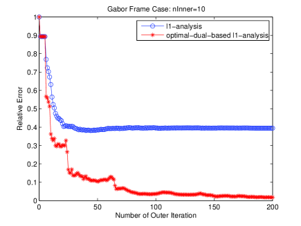
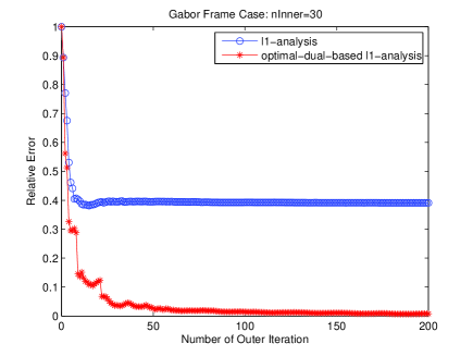
Figure 1: Relative error vs. outer iteration number (without noise). The relative error at iteration $k$ is defined as ${\|{\bf f}-{\bf f}^{k}\|_{2}}/{\|{\bf f}\|_{2}}$, where ${\bf f}^{k}$ is the approximation at iteration $k$ and ${\bf f}$ is the true solution. The optimal-dual-based $\ell_{1}$-analysis problems are solved by Algorithm $1$, while the $\ell_{1}$-analysis problems are by Algorithm $1$ with ${\bf P}{\bf g}\equiv{\bf 0}$. Left: Results for $nInner=10$. Right: Results for $nInner=30$.

Figure 1 shows the relative error vs. outer iteration number for both approaches in noiseless case. It is not hard to see that the optimal-dual-based $\ell_{1}$-analysis approach is more effective than the standard $\ell_{1}$-analysis approach. This is because the optimization of the former is not only over the signal space but also over all dual frames of ${\bf D}$. In other words, there exists some optimal dual frame ${\tilde{\bf D}}_{\text{o}}$ which produces sparser coefficients than the canonical dual frame does for the tested signal. Since ${\tilde{\bf D}}_{\text{o}}$ is also a dual frame, it then follows from (7) that a better recovery performance can be achieved by the optimal-dual-based $\ell_{1}$-analysis approach.

The convergence performance of Algorithm 1 can also be observed in Figure 1. The proposed algorithm converges quickly for the first several iterations, but then slows down as the true solution is near. It is also evident that as $nInner$ increases, the proposed algorithm requires less outer iterations to converge. This is because the subproblem involved in (53) is solved more accurately as $nInner$ increases, the need for outer Bregman updates is naturally less in order to reach the steady state. It is worth noting that as $nInner$ increases, the corresponding complexity for an outer iteration also increases.

Our next simulation is to show the robustness of the optimal-dual-based $\ell_{1}$-analysis with respect to noise in the measurements. Figure 2 shows the recovery error as a function of the noise level. As expected, the relation is linear. We also see that the constant $C_{0}$ in Theorem 1 for the optimal-dual-based $\ell_{1}$-analysis is larger than that for the standard $\ell_{1}$-analysis. But the overall performance of the optimal-dual-based method is still much better.

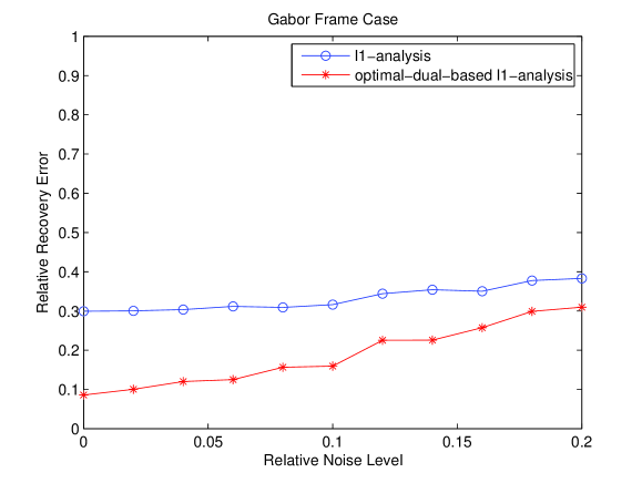
Figure 2: Relative recovery error vs. relative noise level, averaged over $5$ trials. The relative recovery error is defined as ${\|{\bf f}-\hat{{\bf f}}\|_{2}}/{\|{\bf f}\|_{2}}$ and the relative noise level is defined as $\sqrt{m}\sigma/\|\mbox{${\bf\Phi}$}{\bf f}\|_{2}$. The sparsity level is $s=\text{ceil}(0.2\times m)=7$. Set $\lambda=\mu=1$, $tol=10^{-6}$, $nInner=30$, and $nOuter=200$ in Algorithm 1.

We also test the performance of the optimal-dual-based $\ell_{1}$-analysis with respect to the sparsity level of the coefficient vector ${\bf x}$. Figure 3 shows that the optimal-dual-based $\ell_{1}$-analysis outperforms the standard $\ell_{1}$-analysis at different sparsity levels. The plot also shows that the performance curve of the optimal-dual-based $\ell_{1}$-analysis exhibits a threshold effect. When $\varrho\equiv s/m\leq 0.2$, the optimal-dual-based $\ell_{1}$-analysis recovers the signal accurately. When $\varrho\geq 0.2$, the performance degrades as $\varrho$ increases.

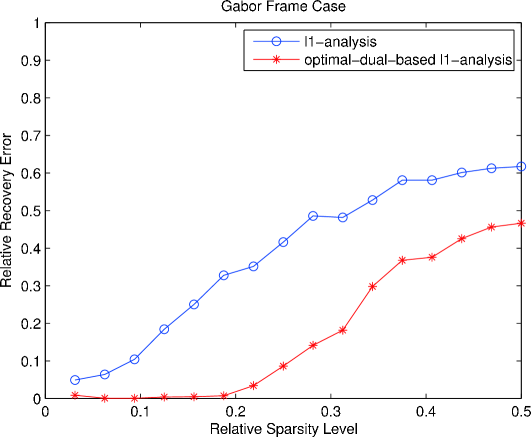
Figure 3: Relative recovery error vs. relative sparsity level of ${\bf x}$, averaged over $100$ trials. The relative recovery error is defined as ${\|{\bf f}-\hat{{\bf f}}\|_{2}}/{\|{\bf f}\|_{2}}$ and the relative sparsity level $\varrho$ is defined as $\varrho=s/m$. No noise $\sigma^{2}=0$. The parameters for Algorithms 1 are the same as in Figure 2.

Example 2: Concatenations.  In many applications, signals of interest are sparse over several orthonormal bases (or frames), it is natural to use a dictionary ${\bf D}$ consisting of a concatenation of these bases (or frames). In this experiment, we consider a dictionary consisting of the coordinate and Fourier bases, i.e., ${\bf D}=[{\bf I},{\bf F}]$. The tested signal ${\bf f}$ is a linear combination of spikes and sinusoids with sparsity $s=\text{ceil}(0.2\times m)=7$. The positions of the nonzero entries of ${\bf x}$ are selected uniformly at random, and each nonzero value is sampled from standard Gaussian distribution. We set $\lambda=\mu=1$, $tol=10^{-12}$ and $nOuter=100$ in Algorithm 1.

Figure 4 shows that the optimal-dual-based $\ell_{1}$-analysis approach achieves much better recovery performance than that of the standard $\ell_{1}$-analysis approach. The latter fundamentally fails with a relative error at about $80\%$. Such a failure is not surprising since ${\bf D}^{*}{\bf f}$ in this case is not at all sparse. This is due to the fact that, in this very example, the component that is sparse in one basis is not at all in the other.

Figures 5 and 6 show the performance of the optimal-dual-based $\ell_{1}$-analysis with respect to the noise level and the sparsity level for the ${\bf I}+{\bf F}$ case, respectively. The results are similar to that for the Gabor frame case. We also see that the standard $\ell_{1}$-analysis fails at all noise levels and sparsity levels in this case.

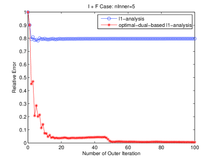
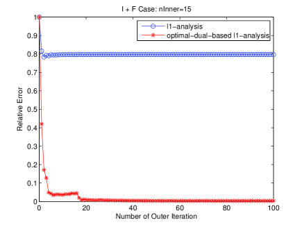
Figure 4: Relative error vs. outer iteration number (without noise). The relative error at iteration $k$ is defined as ${\|{\bf f}-{\bf f}^{k}\|_{2}}/{\|{\bf f}\|_{2}}$, where ${\bf f}^{k}$ is the approximation at iteration $k$ and ${\bf f}$ is the true solution. The optimal-dual-based $\ell_{1}$-analysis problems are solved by Algorithm $1$, while the $\ell_{1}$-analysis problems are by Algorithm $1$ with ${\bf P}{\bf g}\equiv{\bf 0}$. Left: Results for $nInner=5$. Right: Results for $nInner=15$.

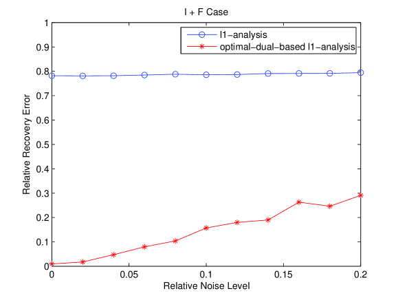
Figure 5: Relative recovery error vs. relative noise level, averaged over $5$ trials. The relative recovery error is defined as ${\|{\bf f}-\hat{{\bf f}}\|_{2}}/{\|{\bf f}\|_{2}}$ and the relative noise level is defined as $\sqrt{m}\sigma/\|\mbox{${\bf\Phi}$}{\bf f}\|_{2}$. The sparsity level is $s=\text{ceil}(0.2\times m)=7$. Set $\lambda=\mu=1$, $tol=10^{-12}$, $nInner=15$, and $nOuter=100$ in Algorithm 1.

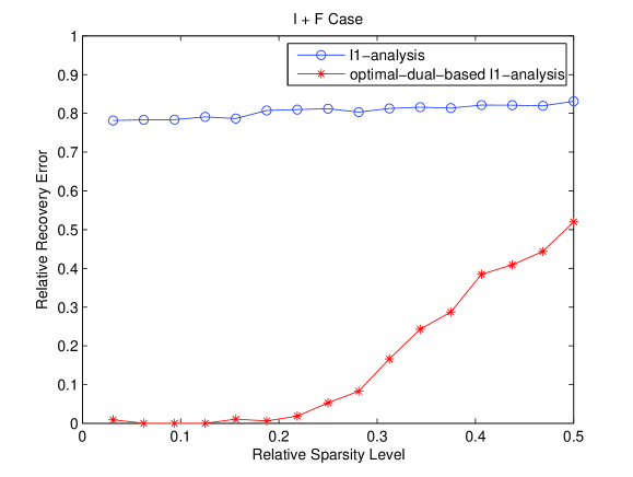
Figure 6: Relative recovery error vs. relative sparsity level of ${\bf x}$, averaged over $100$ trials. The relative recovery error is defined as ${\|{\bf f}-\hat{{\bf f}}\|_{2}}/{\|{\bf f}\|_{2}}$ and the relative sparsity level $\varrho$ is defined as $\varrho=s/m$. No noise $\sigma^{2}=0$. The parameters for Algorithms 1 are the same as in Figure 5.

6 Conclusions

We extend the $\ell_{1}$-analysis approach to a more general case in which the analysis operator can be any dual frame of ${\bf D}$. We call it the general-dual-based approach. Error performance bound is established. Improved sufficient signal recovery conditions are provided. To demonstrate the effectiveness of the general-dual-based approach, we also propose an optimal-dual-based $\ell_{1}$-analysis approach to recover the signal directly. The optimization of this method is not only over the signal space but also over all dual frames of ${\bf D}$. We have seen that when signals are sparse with respect to frames that are redundant and coherent, this optimal-dual-based approach often achieves better recovery performance than that of the standard $\ell_{1}$-analysis. By applying the split Bregman iteration, we develop an iterative algorithm for solving the optimal-dual-based $\ell_{1}$-analysis problem. The proposed algorithm is very fast when proper parameter values are used and easy to code. Our ongoing work includes the performance analysis of the $\ell_{1}$-synthesis approach by virtue of the principle of the optimal-dual-based $\ell_{1}$-analysis approach we proposed, and further refinements of the algorithm.

Appendix A The Basics of the Bregman Iteration

The Bregman iteration is a technique that originated in functional analysis for finding extrema of convex functionals [4]. The Bregman iteration was first introduced to image processing in [32], where it was applied to total variation (TV) denoising. Then, in [6], [34], it was shown to be remarkably successful for $\ell_{1}$ minimization problems in compressed sensing. Here we briefly review this technique. More details about the Bregman iteration can be found in e.g., [6], [7], [32], [34].

The Bregman iteration relies on the concept of the Bregman distance [4]. The Bregman distance of a convex function $J({\bf u})$ between points ${\bf u}$ and ${\bf v}$ is defined as

$$B_{J}^{\bf p}({\bf u},{\bf v})=J({\bf u})-J({\bf v})-\langle{\bf u}-{\bf v},{\bf p}\rangle,$$ (70)

where ${\bf p}\in\partial J({\bf v})$ is some subgradient in the subdifferential of $J$ at the point of ${\bf v}$. Clearly, $B_{J}^{\bf p}({\bf u},{\bf v})$ is not a distance in the usual sense, since $B_{J}^{\bf p}({\bf u},{\bf v})\neq B_{J}^{\bf p}({\bf v},{\bf u})$ in general. However, it does measure the closeness between ${\bf u}$ and ${\bf v}$ in the sense that $B_{J}^{\bf p}({\bf u},{\bf v})\geq 0$ and $B_{J}^{\bf p}({\bf u},{\bf v})\geq B_{J}^{\bf p}({\bf w},{\bf v})$ for all points ${\bf w}$ on the line segment connecting ${\bf u}$ and ${\bf v}$.

First, consider the following unconstrained optimization problem

$$\underset{{\bf u}}{\textrm{min}}\ \ J({\bf u})+H({\bf u}),$$ (71)

where $J({\bf u})$ is some convex function and $H({\bf u})$ is some convex and differentiable function with ${\textrm{argmin}_{\bf u}}H({\bf u})=0$.

Instead of directly solving (71), the Bregman iteration iteratively solves

$${\bf u}^{k+1} =\underset{{\bf u}}{\textrm{argmin}}\ \ B_{J}^{{\bf p}^{k}}({\bf u},{\bf u}^{k})+H({\bf u}),$$

$$=\underset{{\bf u}}{\textrm{argmin}}\ \ J({\bf u})-J({\bf u}^{k})-\langle{\bf u}-{\bf u}^{k},{\bf p}^{k}\rangle+H({\bf u}),$$ (72)

for $k=0,1,\ldots,$ starting from ${\bf u}^{0}={\bf 0}$ and ${\bf p}^{0}={\bf 0}$. In (A), the updating formula for ${\bf p}^{k}$ is based on the optimality conditions of (A). Since ${\bf u}^{k+1}$ minimizes (A), then $0\in\partial\{B_{J}^{{\bf p}^{k}}({\bf u},{\bf u}^{k})+H({\bf u})\}$, where this subdifferential is evaluated at ${\bf u}^{k+1}$, i.e.,

$$0\in\partial J({\bf u}^{k+1})-{\bf p}^{k}+\nabla H({\bf u}^{k+1}).$$

This leads to

$${\bf p}^{k+1}={\bf p}^{k}-\nabla H({\bf u}^{k+1})\in\partial J({\bf u}^{k+1}).$$ (73)

Combining (A) and (73) yields the Bregman iteration:

$$\left\{\begin{array}[]{l}{\bf u}^{k+1}={\textrm{argmin}_{\bf u}}B_{J}^{{\bf p}^{k}}({\bf u},{\bf u}^{k})+H({\bf u}),\\ {\bf p}^{k+1}={\bf p}^{k}-\nabla H({\bf u}^{k+1}),\end{array}\right.$$ (74)

for $k=0,1,\ldots,$ starting with ${\bf u}^{0}={\bf 0}$ and ${\bf p}^{0}={\bf 0}$.

The convergence of the Bregman iteration (74) was analyzed in [32]. In particular, it was shown that, under fairly weak assumptions on $J({\bf u})$ and $H({\bf u})$, $H({\bf u}^{k})\rightarrow 0$ as $k\rightarrow\infty$.

We then show that the Bregman iteration can also be used to solve the general constrained convex minimization problem:

$$\underset{{\bf u}}{\textrm{min}}\ \ J({\bf u})\ \ s.t.\ \ \mbox{${\bf\Phi}$}{\bf u}={\bf y},$$ (75)

where $J({\bf u})$ denotes some convex function and ${\bf\Phi}$ is some linear operator.

Traditionally, this problem may be solved by a continuation method, where we solve sequentially the unconstrained problems

$$\underset{{\bf u}}{\textrm{min}}\ \ J({\bf u})+\frac{\lambda_{k}}{2}\|\mbox{${\bf\Phi}$}{\bf u}-{\bf y}\|_{2}^{2},$$ (76)

where $\lambda_{1}<\lambda_{2}<\ldots<\lambda_{K}$ is an increasing sequence of penalty function weights [3]. In order to enforce that $\mbox{${\bf\Phi}$}{\bf u}\approx{\bf y}$, we must choose $\lambda_{K}$ to be extremely large. However, choosing a large value for $\lambda_{k}$ may make (76) extremely difficult to solve numerically [23].

The Bregman iteration provides another way to transfer the constrained problem (75) into a series of unconstrained problems. To this end, we first convert (75) into an unconstrained optimization problem using a quadratic penalty function:

$$\underset{{\bf u}}{\textrm{min}}\ \ J({\bf u})+\frac{\lambda}{2}\|\mbox{${\bf\Phi}$}{\bf u}-{\bf y}\|_{2}^{2}.$$ (77)

Then we apply the Bregman iteration (74) and iteratively minimize:

$$\left\{\begin{array}[]{l}{\bf u}^{k+1}={\textrm{argmin}_{\bf u}}B_{J}^{{\bf p}^{k}}({\bf u},{\bf u}^{k})+\frac{\lambda}{2}\|\mbox{${\bf\Phi}$}{\bf u}-{\bf y}\|_{2}^{2},\\ {\bf p}^{k+1}={\bf p}^{k}-\lambda\mbox{${\bf\Phi}$}^{*}(\mbox{${\bf\Phi}$}{\bf u}^{k+1}-{\bf y}),\end{array}\right.$$ (78)

for $k=0,1,\ldots,$ starting with ${\bf u}^{0}={\bf 0}$ and ${\bf p}^{0}={\bf 0}$.

By change of variable, this seemingly complicated iteration (78) can be reformulated into a simplified form [7]:

$$\left\{\begin{array}[]{l}{\bf u}^{k+1}={\textrm{argmin}_{{\bf u}}}J({\bf u})+\frac{\lambda}{2}\|\mbox{${\bf\Phi}$}{\bf u}-{\bf y}+{\bf b}^{k}\|_{2}^{2},\\ {\bf b}^{k+1}={\bf b}^{k}+(\mbox{${\bf\Phi}$}{\bf u}^{k+1}-{\bf y}),\end{array}\right.$$ (79)

for $k=0,1,\ldots,$ starting with ${\bf b}^{0}=0$ and ${\bf u}^{0}=0$.

Indeed, by ${\bf p}^{0}={\bf 0}$ and induction on ${\bf p}^{k}$, we obtain ${\bf p}^{k}=-\lambda\mbox{${\bf\Phi}$}^{*}\sum_{j=1}^{k}(\mbox{${\bf\Phi}$}{\bf u}^{j}-{\bf y})$. Substituting this into the first step of (78) yields

$$B_{J}^{{\bf p}^{k}}({\bf u},{\bf u}^{k})+\frac{\lambda}{2}\|\mbox{${\bf\Phi}$}{\bf u}-{\bf y}\|_{2}^{2} =J({\bf u})-J({\bf u}^{k})-\langle{\bf u}-{\bf u}^{k},{\bf p}^{k}\rangle+\frac{\lambda}{2}\|\mbox{${\bf\Phi}$}{\bf u}-{\bf y}\|_{2}^{2}$$

$$=J({\bf u})-\langle{\bf u},{\bf p}^{k}\rangle+\frac{\lambda}{2}\|\mbox{${\bf\Phi}$}{\bf u}-{\bf y}\|_{2}^{2}+C_{2}$$

$$=J({\bf u})+\lambda\langle\mbox{${\bf\Phi}$}{\bf u},\sum_{j=1}^{k}(\mbox{${\bf\Phi}$}{\bf u}^{j}-{\bf y})\rangle+\frac{\lambda}{2}\|\mbox{${\bf\Phi}$}{\bf u}-{\bf y}\|_{2}^{2}+C_{2}$$

$$=J({\bf u})+\frac{\lambda}{2}\left\|\mbox{${\bf\Phi}$}{\bf u}-{\bf y}+\sum_{j=1}^{k}(\mbox{${\bf\Phi}$}{\bf u}^{j}-{\bf y})\right\|_{2}^{2}+C_{3},$$ (80)

where $C_{2}$ and $C_{3}$ are independent of ${\bf u}$. By the definition of ${\bf u}^{k+1}$ in (78), we have that

$${\bf u}^{k+1}=\underset{{\bf u}}{\textrm{argmin}}\ \ J({\bf u})+\frac{\lambda}{2}\left\|\mbox{${\bf\Phi}$}{\bf u}-{\bf y}+\sum_{j=1}^{k}(\mbox{${\bf\Phi}$}{\bf u}^{j}-{\bf y})\right\|_{2}^{2}.$$ (81)

Define ${\bf b}^{k}=\sum_{j=1}^{k}(\mbox{${\bf\Phi}$}{\bf u}^{k}-{\bf y})$, then we have

$${\bf b}^{k+1}={\bf b}^{k}+(\mbox{${\bf\Phi}$}{\bf u}^{k+1}-{\bf y}),\ \ {\bf b}^{0}={\bf 0}.$$ (82)

With this, (81) becomes

$${\bf u}^{k+1}=\underset{{\bf u}}{\textrm{argmin}}\ \ J({\bf u})+\frac{\lambda}{2}\|\mbox{${\bf\Phi}$}{\bf u}-{\bf y}+{\bf b}^{k}\|_{2}^{2}.$$ (83)

Combining (83) and (82) yields (79). It is this form (79) that will be used to derive the split Bregman iteration.

The convergence results of the Bregman iteration (78) (or (79)) were given in [23], [34]. It was shown that the sequence ${\bf u}^{k}$ generated by (78) (or (79)) weakly converges to a solution of (75).

References

- [1] R. Baraniuk, M. Davenport, R. DeVore, and M. Wakin, “A simple proof of the restricted isometry property for random matrices,” Constr. Approx., vol. 28, pp. 253–263, 2008.
- [2] S. Becker, J. Bobin, and E. J. Candès, “NESTA: a fast and accurate first-order method for sparse recovery” SIAM J. Imag. Sci., vol. 4, no. 1, pp. 1–39, 2011.
- [3] S. Boyd and L. Vandenberghe, Convex Optimization. Cambridge, U.K.: Cambridge Univ. Press, 2004.
- [4] L. Bregman, “The relaxation method of finding the common points of convex sets and its application to the solution of problems in convex optimization,” USSR Comput. Math. and Math. Phys., vol. 7, pp. 200–217, 1967.
- [5] A. M. Bruckstein, D. L. Donoho, and M. Elad, “From sparse solutions of systems of equations to sparse modeling of signals and images,” SIAM Rev., vol. 51, pp. 34–81, 2009.
- [6] J. Cai, S. Osher, and Z. Shen, “Linearized Bregman iterations for compressed sensing,” Math. Comp., vol. 78, pp. 1515–1536, 2009.
- [7] J. Cai, S. Osher, and Z. Shen, “Split Bregman methods and frame based image restoration,” SIAM J. Multiscale Model. Simul., vol. 8, pp. 337–369, 2009.
- [8] T. Cai, G. Xu, and J. Zhang, “On recovery of sparse signals via minimization,” IEEE Trans. Inf. Theory, vol. 55, pp. 3388–3397, July, 2009.
- [9] T. Cai, L. Wang, and G. Xu, “Shifting inequality and recovery of sparse signals,” IEEE Trans. Signal Process., vol. 58, pp. 1300–1308, Mar., 2010.
- [10] E. J. Candès and T. Tao, “Decoding by linear programming,” IEEE Trans. Inf. Theory, vol. 51, pp. 4203–4215, Dec., 2005.
- [11] E. J. Candès, J. Romberg, and T. Tao, “Stable signal recovery from incomplete and inaccurate measurements,” Comm. Pure Appl. Math., vol. 59, pp. 1207–1223, 2006.
- [12] E. J. Candès and T. Tao, “Near optimal signal recovery from random projections: Universal encoding strategies?,” IEEE Trans. Inf. Theory, vol. 52, pp. 5406–5425, Dec., 2006.
- [13] E. J. Candès, J. Romberg, and T. Tao, “Robust uncertainty principles: exact signal reconstruction from highly incomplete frequency information,” IEEE Trans. Inf. Theory, vol. 52, pp. 489–509, Feb., 2006.
- [14] E. J. Candès, “Compressive sampling,” in Proc. Int. Cong. Mathematicians, Madrid, Spain, vol. 3, pp. 1433–1452, 2006.
- [15] E. J. Candès, Y. C. Eldar, D. Needell, and P. Randall, “Compressed sensing with coherent and redundant dictionaries,” Appl. Computat. Harmon. Anal., 2011, to appear. [Online]. Available: http://arxiv.org/abs/1005.2613
- [16] S. S. Chen, D. L. Donoho, and M. A. Saunders, “Atomic decomposition by basis pursuit,” SIAM Rev., vol. 43, pp. 129–159, 2001.
- [17] O. Chiristensen, An Introduction to Frames and Riesz Bases. Boston, MA: Birkhäuser, 2003, pp. 87–121.
- [18] D. L. Donoho, “Compressed sensing,” IEEE Trans. Inf. Theory, vol. 52, pp. 1289–1306, Apr., 2006.
- [19] D. L. Donoho, M. Elad, and V. N. Temlyakov, “Stable recovery of sparse overcomplete representations in the presence of noise,” IEEE Trans. Inf. Theory, vol. 52, pp. 6–18, Jan., 2006.
- [20] M. Elad, J. L. Starck, P. Querre, and D. L. Donoho, “Simultaneous cartoon and texture image inpainting using morphological component analysis (MCA),” Appl. Computat. Harmon. Anal., vol. 19, pp. 340–358, 2005.
- [21] M. Elad, P. Milanfar, and R. Rubinstein, “Analysis versus synthesis in signal priors,” Inverse Probl., vol. 23, pp. 947–968, 2007.
- [22] S. Foucart, “A note on guaranteed sparse recovery via -minimization,” Appl. Computat. Harmon. Anal., vol. 29, pp. 97–103, 2010.
- [23] T. Goldstein and S. Osher, “The split Bregman algorithm for L1-regularized problems,” SIAM J. Imag. Sci., vol. 2, pp. 323–343, 2009.
- [24] D. Han, K. Kornelson, D. Larson, and Eric Weber, Frames for Undergraduates. Providence, RI: American Mathematical Society, 2007.
- [25] C. E. Heil and D. F. Walnut, “Continuous and discrete wavelet transforms,” SIAM Rev., vol. 31, pp. 628–666, 1989.
- [26] W. B. Johnson and J. Lindenstrauss, “Extensions of Lipschitz mappings into a Hilbert space,” Contemp. Math, vol. 26, pp. 189–206, 1984.
- [27] F. Krahmer and R. Ward, ”New and improved Johnson-Lindenstrauss embeddings via the Restricted Isometry Property,” SIAM J. Math. Anal., vol. 43, pp. 1269–1281, 2011.
- [28] S. Li, “On general frame decompositions,” Numer. Funct. Anal. Optim., vol. 16, pp. 1181–1191, 1995.
- [29] S. Mallat and Z. Zhang, “Matching pursuits with time-frequency dictionaries,” IEEE Trans. Signal Process., vol. 41, pp. 3397–3415, Dec., 1993.
- [30] S. Mallat, A Wavelet Tour of Signal Processing. San Diego: Academic Press, 1998.
- [31] D. Needell and J. Tropp, “CoSaMP: Iterative signal recovery from incomplete and inaccurate samples,” Appl. Computat. Harmon. Anal., vol. 26, pp. 301–321, May, 2009.
- [32] S. Osher, M. Burger, D. Goldfarb, J. Xu, and W. Yin, “An iterative regularization method for total variation-based image restoration,” SIAM J. Multiscale Model. Simul., vol. 4, pp. 460– 489, 2005.
- [33] H. Rauhut, K. Schnass, and P. Vandergheynst, ”Compressed sensing and redundant dictionaries,” IEEE Trans. Inf. Theory, vol. 54, pp. 2210–2219, May, 2008.
- [34] W. Yin, S. Osher, D. Goldfarb, and J. Darbon, “Bregman iterative algorithms for - minimization with applications to compressed sensing,” SIAM J. Imag. Sci., vol. 1, pp. 143–168, 2008.