Classification of Arbitrary Multipartite Entangled States under Local Unitary Equivalence

Abstract

We propose a practical method for finding the canonical forms of arbitrary dimensional multipartite entangled states, either pure or mixed. By extending the technique developed in one of our recent works, the canonical forms for the mixed $N$-partite entangled states are constructed where they have inherited local unitary symmetries from their corresponding $N+1$ pure state counterparts. A systematic scheme to express the local symmetries of the canonical form is also presented, which provides a feasible way of verifying the local unitary equivalence for two multipartite entangled states.

PACS numbers: 03.67.Mn, 03.65.Ud, 02.10.Xm

1 Introduction

Entanglement is one of the most important ingredients in quantum information science; it gives impetus to the most extraordinary nonclassical applications, such as teleportation and quantum computation, etc [1]. It is now generally regarded that the entanglement is a key physical resource in realizing many quantum information tasks, thus the quantitative and qualitative study of entanglement become more and more important. Though superficially entangled states show different features—usually not all entangled states are functionally independent—they may be intrinsically the same as far as the entanglement property is concerned. Two entangled states are said to be equivalent in implementing the same quantum information task if they can be obtained with certainty from each other via local operation and classical communication (LOCC). Theoretically, this LOCC equivalent class is such defined that within the class any two quantum states are inter-convertible by local unitary (LU) operators [2].

The characterization of bipartite entangled states under LU equivalence can be well understood by using the singular value (Schmidt) decomposition. However things turn out to be much more complicated when the multipartite states are concerned. On one hand, the characterization of multipartite entanglement can be done by computing the local unitary invariants of the quantum states [3]. Two entangled states are LU equivalent if they have the same LU invariants; the relation between LU equivalence for $n$-partite pure states and the $(n-1)$-partite mixed states has also been observed and is used in constructing the local unitary invariants [4, 5]. The parameters in local invariants grow dramatically as the number of partite increases, and the problem of identifying and interpreting independent invariants becomes very complicated [6]. Recently a operationally meaningful measures has been introduced for three-qubit entanglement [7]. On the other hand, one can chose certain bases and put the quantum states in some canonical (standard) forms. Along this line, a canonical method was proposed in Ref.[8], though it was only given in a set of constraints on the coefficients of the quantum state. Later, this method was reformulated into a compact form [9]. By introducing the standard form for multipartite states, Kraus proposed a general way to determine the LU transformation between two LU equivalent $n$-qubit states [10, 11], however as the dimension increases, degeneracy emerges between the identical eigenvalues of the one partite reduced density matrix, and the verification of LU equivalence becomes unpractical.

Recently, in [12] we have proposed a practical method for finding the canonical form of pure multipartite state by using the high order singular value decompositions (HOSVDs) and the local symmetry properties of the tensor form quantum states. In this work, we generalize this method to the mixed states where the canonical forms for arbitrary mixed multipartite states are constructed. Also, we develop a systematic scheme to present the local symmetries among the canonical forms, which provides a feasible way to verify the LU equivalence of two quantum states regardless of the degeneracy conditions.

The structure of the paper goes as follows. In section 2, we give a brief introduction to the basic technique of HOSVD which is used in our entanglement classification. In section 3, we reformulate the entanglement classification for multipartite pure states under LU equivalence in a neater form, and a practical classification method for arbitrary multipartite mixed states is developed where the canonical forms for mixed states are explicitly constructed. After this complete classification of multipartite entangled states with their canonical forms, in section 4 we develop a systematic scheme for verifying the LU symmetry between two entangled states. In section 5, practical examples of three- and four-qubit states are given. Finally, some concluding remarks are presented in section 6.

2 LU equivalence of multipartite quantum state

A general $N$-partite entangled quantum state in the dimensions $I_{1}\times I_{2}\times\cdots\times I_{N}$ can be formulated in the following form:

$$|\Psi\rangle=\sum_{i_{1}=1,i_{2}=1,...,i_{N}=1}^{I_{1},I_{2},\cdots,I_{N}}\psi_{i_{1}i_{2}...i_{N}}|i_{1}\rangle|i_{2}\rangle...|i_{N}\rangle\;,$$ (1)

where $\psi_{i_{1}i_{2}...i_{N}}\in\mathbb{C}$ are coefficients of the quantum state in representative bases. Two quantum states are said to be LU equivalent if they are inter-convertible by LU operators, which can be schematically expressed as

$$|\Psi^{\prime}\rangle = \bigotimes_{i}^{N}U^{(i)}|\Psi\rangle$$ (2)

$$= \sum_{\begin{subarray}{c}i_{1},i_{2},\cdots,i_{N}\\ i^{\prime}_{1},i^{\prime}_{2},\cdots,i^{\prime}_{N}\end{subarray}}\psi_{i_{1}i_{2}\cdots i_{N}}u^{(1)}_{i^{\prime}_{1}i_{1}}|{i^{\prime}_{1}\rangle u^{(2)}_{i^{\prime}_{2}i_{2}}|i^{\prime}_{2}\rangle\cdots u^{(N)}_{i^{\prime}_{N}i_{N}}|i^{\prime}_{N}}\rangle\;$$

$$= \sum_{i_{1},i_{2},\cdots,i_{N}}\psi^{\prime}_{i_{1}i_{2}\cdots i_{N}}|{i_{1},i_{2},\cdots,i_{N}}\rangle\;.$$

Here, the coefficients $\psi_{i_{1}i_{2}...i_{N}}$ can also be treated as the entries of a tensor $\Psi$ and hence the quantum states can be represented by high order complex tensors. In the tensor form of $\Psi$, the unitary operator $U^{(n)}$ acting on the $n$th partite is defined as

$$(U^{(n)}\Psi)_{i_{1}i_{2}\cdots i_{n-1}i_{n}^{\prime}i_{n+1\cdots i_{N}}}\equiv\sum_{i_{n}}\psi_{i_{1}i_{2}\cdots i_{n-1}i_{n}i_{n+1}\cdots i_{N}}u^{(n)}_{i^{\prime}_{n}i_{n}}\;.$$ (3)

For bipartite pure state, the tensor $\Psi$ is a matrix $\Psi=[\psi_{i_{1}i_{2}}]\in\mathbb{C}^{I_{1}\times I_{2}}$ (matrices with complex numbers of $I_{1}$ rows and $I_{2}$ columns) where the dimensions of the Hilbert space for each partite are $I_{1}$ and $I_{2}$ separately. The singular value decomposition (SVD) of the bipartite state $\Psi$ of dimensions $I_{1}\times I_{2}$ reads

$$\Lambda=U^{(1)}\cdot\Psi\cdot U^{(2)}=\mathrm{diag}\{\lambda_{1},\cdots,\lambda_{I}\}\;,$$ (4)

where $\lambda_{i}\geq\lambda_{j}\geq 0,\forall\,i<j$, $I=\mathrm{min}\{I_{1},I_{2}\}$. $\Lambda$ has the following two properties:

1. the singular values $\lambda_{i},i\in\{1,\cdots,I\}$ of matrix $\Psi$ are uniquely defined.

2. $\Lambda$ is a diagonal matrix and uniquely defined (with prescribed order of the singular values).

In this case, the singular values of the quantum state $\Psi$ readily characterize its entanglement properties under LU equivalence. Two bipartite quantum states are LU equivalent if, and only if, they have the same SVDs.

Here we introduce the technique which can be seen as the generalization of SVD to high dimensional multipartite systems–the HOSVD [13]. Let us define the matrix unfolding of the tensor $\Psi\in\mathbb{C}^{I_{1}I_{2}\cdots I_{N}}$ with $n$th index as

$$\Psi_{(n)}\in\mathbb{C}^{I_{n}\times(I_{n+1}I_{n+2}\cdots I_{N}I_{1}I_{2}\cdots I_{n-1})}\;.$$ (5)

Here $\Psi_{(n)}$ is a $I_{n}\times(I_{n+1}I_{n+2}\cdots I_{N}I_{1}I_{2}\cdots I_{n-1})$ matrix. For example, the $2\times 3\times 4$ complex tensor $\Psi$, unfolding with the second and third indexes, has the following forms:

$$\Psi_{(2)} = \begin{pmatrix}\psi_{111}&\psi_{211}&\psi_{112}&\psi_{212}&\psi_{113}&\psi_{213}&\psi_{114}&\psi_{214}\\ \psi_{121}&\psi_{221}&\psi_{122}&\psi_{222}&\psi_{123}&\psi_{223}&\psi_{124}&\psi_{224}\\ \psi_{131}&\psi_{231}&\psi_{132}&\psi_{232}&\psi_{133}&\psi_{233}&\psi_{134}&\psi_{234}\end{pmatrix}\;,$$

$$\Psi_{(3)} = \begin{pmatrix}\psi_{111}&\psi_{121}&\psi_{131}&\psi_{211}&\psi_{221}&\psi_{231}\\ \psi_{112}&\psi_{122}&\psi_{132}&\psi_{212}&\psi_{222}&\psi_{232}\\ \psi_{113}&\psi_{123}&\psi_{133}&\psi_{213}&\psi_{223}&\psi_{233}\\ \psi_{114}&\psi_{124}&\psi_{134}&\psi_{214}&\psi_{224}&\psi_{234}\end{pmatrix}\;.$$ (6)

For arbitrary $N$-partite systems there exists a core tensor $\Omega$ for each tensor $\Psi$,

$$\Omega=U^{(1)}\otimes U^{(2)}\otimes\cdots\otimes U^{(N)}\Psi\;.$$ (7)

Here $\Omega$ is a same order tensor as $\Psi$ in the Hilbert space of $I_{1}\times I_{2}\times\cdots\times I_{N}$. Any $N$-$1$ order tensor $\Omega_{i_{n}=i}$ obtained by fixing the $n$th index to $i$, has the following property:

$$\langle\Omega_{i_{n}=i},\Omega_{i_{n}=j}\rangle=\delta_{\scriptstyle ij}\,\left(\sigma_{i}^{(n)}\right)^{2}\;,$$ (8)

where $\sigma_{i}^{(n)}$ is called the $n$-mode singular value of $\Psi$ and $\sigma_{i}^{(n)}\geq\sigma_{j}^{(n)}\geq 0$, $\forall\;i<j$ . The singular value $\sigma_{i}^{(n)}$ symbolizes the Frobenius-norm $\sigma_{i}^{(n)}=||\Omega_{i_{n}=i}||\equiv\sqrt{\langle\Omega_{i_{n}=i},\Omega_{i_{n}=i}\rangle}$, where the inner product $\langle\mathcal{A},\mathcal{B}\rangle\equiv\sum_{i_{1}}\sum_{i_{2}}\cdot\cdot\cdot\sum_{i_{N}}b_{i_{1}i_{2}...i_{N}}a^{*}_{i_{1}i_{2}...i_{N}}$ (see [13] for details).

In the following we show how to get the core tensor by the LU transformation $U^{(i)},i\in\{1,\cdots,N\}$ in Eq.(7). A quantum state $\Omega$ with the same dimension as $\Psi$ is LU equivalent to $\Psi$ if

$$\Omega=U^{(1)}\otimes U^{(2)}\otimes\cdots\otimes U^{(N)}\Psi\;,$$ (9)

where $U^{(i)},i\in\{1,\cdots,N\}$ are unitary matrices. In the matrix unfolding form, Eq.(9) can be rewritten as

$$\Omega_{(n)}=U^{(n)}\cdot\Psi_{(n)}\cdot(U^{(n+1,\cdots,n-1)})^{\mathrm{T}}\;.$$ (10)

Here $U^{(n+1,\cdots n-1)}\equiv U^{(n+1)}\otimes U^{(n+2)}\otimes\cdots\otimes U^{(N)}\otimes U^{(1)}\otimes\cdots\otimes U^{(n-1)}$; $\Omega_{(n)}$ and $\Psi_{(n)}$ have the same dimensions: $I_{n}$ rows and $(I_{n+1}\times I_{n+2}\cdots\times I_{N}\times I_{1}\times\cdots\times I_{n-1})$ columns. Now consider the particular case where $U^{(n)}$ is obtained from the singular value decomposition of matrix $\Psi_{(n)}$, i.e.

$$U^{(n)}\cdot\Psi_{(n)}\cdot V^{(n)}=\mathrm{diag}\{\sigma_{1}^{(n)},\sigma_{2}^{(n)},\cdots,\sigma_{I_{n}}^{(n)}\}\;,$$ (11)

where $U^{(n)}$ and $V^{(n)}$ are unitary matrix, and $\sigma_{i}^{(n)}\geq\sigma_{j}^{(n)}\geq 0,\forall\,i<j$. Eq.(10) now can be written as

$$\Omega_{(n)}=\mathrm{diag}\{\sigma_{1}^{(n)},\sigma_{2}^{(n)},\cdots,\sigma_{I_{n}}^{(n)}\}\cdot V^{(n){\dagger}}\cdot(U^{(n+1,\cdots,n-1)})^{\mathrm{T}}\;.$$ (12)

It is clear that $\Omega_{(n)}$ has orthogonal rows

$$\langle\Omega_{i_{n}=j},\Omega_{i_{n}=k}\rangle=\delta_{jk}\,\left(\sigma_{j}^{(n)}\right)^{2}\;.$$ (13)

Eq.(13) always holds if $U^{(n+1,\cdots,n-1)}$ is a unitary matrix. In the similar way we can obtain all the other local unitary matrices $U^{(i)},i\in\{1,2,\cdots,N\}$, and eventually, the core tensors $\Omega$ of $\Psi$ can then be constructed via Eq.(9).

From the construction of the core tensor, two of the important properties of HOSVD (when compared to its bipartite counterpart) can be concluded:

1. The $n$-mode singular values $\sigma_{i}^{(n)},i\in\{1,\cdots,I_{n}\},n\in\{1,\cdots,N\}$, of $\Psi$ are uniquely defined.

2. If $\forall\,n\in\{1,\cdots,N\}$ the $n$-mode singular values $\sigma_{i}^{(n)}$ are all distinct, then $\Omega^{\prime}_{(n)}=\Theta_{(n)}\Omega_{(n)}$ is also a HOSVD of $\Psi$ where $\Theta_{(n)}=\mathrm{diag}\{e^{i\theta_{1}^{(n)}},\cdots,e^{i\theta_{I_{n}}^{(n)}}\}$. Otherwise, let $\sigma_{1}^{(n)}>\sigma_{2}^{(n)}>\cdots>\sigma_{k_{n}}^{(n)}\geq 0$ denote the distinct $n$-mode singular values of $\Omega_{(n)}$ with respective positive multiplicities $\mu_{1}^{(n)},\mu_{2}^{(n)},\cdots,\mu_{k_{n}}^{(n)}$ where $\sum_{i=1}^{k_{n}}\mu^{(n)}_{i}=I_{n}$. In this case,

   $$\Omega^{\prime}_{(n)}=\left[\bigoplus_{i=1}^{k_{n}}u^{(n)}_{i}\right]\,\Omega_{(n)}\equiv S^{(n)}\,\Omega_{(n)}$$ (14)

   is also a HOSVD of $\Psi$. Here $u^{(n)}_{i}\in\mathbb{C}^{\mu^{(n)}_{i}\times\mu^{(n)}_{i}}$ are arbitrary $\mu^{(n)}_{i}\times\mu^{(n)}_{i}$ unitary matrices and constitute the diagonal blocks of $S^{(n)}$ which are conformal to those $n$-mode singular values of $\Omega_{n}$ with multiplicity.

From the second property it is clear that, unlike the bipartite case, the core tensor $\Omega$ (HOSVD) of $\Psi$ is not uniquely defined.

3 Classification under local unitary equivalence

In this section we propose entanglement classification scheme by decomposing the LU equivalence of the quantum states into two correlated problems: the HOSVD and LU symmetries. First, we give a brief introduction to the entanglement classification of arbitrary dimensional multipartite pure states which was first proposed in [12], then we extend the method to the mixed states, by which the canonical forms for entanglement classes of mixed states under the LU equivalence can be constructed neatly.

3.1 LU equivalence for multipartite pure states

Due to the nonuniqueness of the core tensors, $\Omega$ can not be identified as the entanglement classes of the quantum states. The philosophy of our scheme in [12] is that if we impose this nonuniqueness as a local symmetry within the core tensors themselves, then we can get the unique canonical forms. That is, if we regard the core tensors $\Omega$ and $\Omega^{\prime}$ which are related by LU operators as the same entanglement class then the HOSVD can be seen as the entanglement classification of the multipartite state $\Psi$.

Suppose that the core tensor $\Omega$ have $k_{n}$ distinct $n$-mode singular values $\sigma_{i}^{(n)},i\in\{1,2,\cdots,k_{n}\}$, each with multiplicity of $\mu_{i}^{(n)}$ where $\sum_{i=1}^{k_{n}}\mu^{(n)}_{i}=I_{n}$. Here we regard these multiplicities as the degeneracies of the singular values which corresponds to the case of nongeneric states of [10]. From Eq.(14) we can infer that the LU symmetry which relates two core tensors takes the following form

$$S=\bigotimes_{n=1}^{N}\left[\bigoplus_{i=1}^{k_{n}}u_{i}^{(n)}\right]\;.$$ (15)

The core tensors $\Omega^{\prime}$ and $\Omega$ related by this symmetry now can be written as

$$\Omega^{\prime}=S\,\Omega\;.$$ (16)

Two different core tensors related by $S$ belong to the same entanglement class. We can call such core tensor $\Omega$ of $\Psi$ associated with corresponding local symmetry $S$ the canonical form of $\Psi$.

In order to see how this symmetry act on the core tensors we introduce the technique of vectorization of the matrix. With each matrix $A=[a_{ij}]\in\mathbb{C}^{I_{1}\times I_{2}}$, we can associated it with a vector $\vec{A}$ defined by

$$\vec{A}\equiv\left[a_{11},\cdots,a_{I_{1}1},a_{12},\cdots,a_{I_{1},2},\cdots,a_{1I_{2}},\cdots,a_{I_{1}I_{2}}\right]^{\mathrm{T}}\;.$$ (17)

Two tensors $\Psi$ and $\Psi^{\prime}$ of $I_{1}\times I_{2}\times\cdots I_{N}$ which are related by local operators $U^{(n)},n\in\{1,2,\cdots,N\}$, can be expressed in the matrix unfolding form with the $n$th index

$$\Psi^{\prime}_{(n)}=U^{(n)}\cdot\Psi_{(n)}\cdot(U^{(n+1)}\otimes U^{(n+2)}\otimes\cdots\otimes U^{(N)}\otimes U^{(1)}\otimes\cdots\otimes U^{(n-1)})^{\mathrm{T}}\;,$$ (18)

With the convention of Eq.(17), the matrix equation Eq.(18), can be written as (see [14])

$$U^{(n+1)}\otimes U^{(n+2)}\otimes\cdots\otimes U^{(N)}\otimes U^{(1)}\otimes\cdots\otimes U^{(n-1)}\otimes U^{(n)}\vec{\Psi}_{(n)}=\,\vec{\Psi}^{\prime}_{(n)}\;.$$ (19)

This can be seen as a unitary transformation of a $I_{1}\times I_{2}\times\cdots\times I_{N}$ vector $\vec{\Psi}_{(n)}$ to $\vec{\Psi}^{\prime}_{(n)}$. On choosing $n=N$, we have the simple form of Eq.(19)

$$U^{(1)}\otimes\cdots\otimes U^{(N)}\vec{\Psi}_{(N)}=\,\vec{\Psi}^{\prime}_{(N)}\;.$$ (20)

Here the symmetry between their core tensors, Eq.(16), can be similarly represented as

$$\vec{\Omega^{\prime}}_{(N)}=S\,\vec{\Omega}_{(N)}\equiv\bigotimes_{n=1}^{N}\left[\bigoplus_{i=1}^{k_{n}}u_{i}^{(n)}\right]\vec{\Omega}_{(N)}\;,$$ (21)

where $u_{i}^{(n)}$ is a $\mu_{i}^{(n)}\times\mu_{i}^{(n)}$ unitary matrix and $\sum_{i=1}^{k_{n}}\mu_{i}^{(n)}=I_{n}$. In the blocks diagonalized form, Eq.(21) is

$$\begin{pmatrix}u^{(1)}_{1}\otimes\cdots\otimes u^{(N)}_{1}&0&\cdots&0\\ 0&u^{(1)}_{1}\otimes\cdots\otimes u^{(N)}_{2}&\cdots&0\\ \vdots&\vdots&\ddots&\vdots\\ 0&0&\cdots&u^{(1)}_{k_{1}}\otimes\cdots\otimes u^{(N)}_{k_{N}}\end{pmatrix}\cdot\vec{\Omega}_{(N)}=\vec{\Omega^{\prime}}_{(N)}\;.$$ (22)

We can set $u^{(n)}_{j}=e^{i\theta_{j}^{(n)}}$ if the multiplicity $\mu^{(n)}_{j}=1$. In all, we have the following theorem which has been state in [12]

Theorem 1

The core tensors $\Omega$ associated with the local symmetry group $S$ is the canonical form of the multipartite pure state and is the entanglement class under LU equivalence.

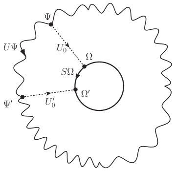
Figure 1: The wiggled line represents $U\Psi$ and it forms an orbit with irregular shapes; the circle line represents $S\Omega$ and it forms well-structured orbit. $\Omega=U_{0}\Psi$ and $\Omega^{\prime}=U_{o}^{\prime}\Psi^{\prime}$ both are the core tensors on the $S\Omega$ orbit.

From this theorem, we can form a more general point of view for the equivalent entanglement class. Any subset of the quantum states in $I_{1}\times I_{2}\times\cdots\times I_{N}$, i.e., $\{\psi\}$, associated with its local unitary transformation group $U=\bigotimes_{i}U^{(i)}$ where $\{\psi|U\psi\in\{\psi\}\}$ can be regarded as a unique representation of entanglement class. Let $\{\Psi,U\}$ be such subset of the quantum states associated with its LU symmetry, then it would be intrinsically the same as the classification with the HOSVD $\Omega$ and its LU symmetry group $S$, i.e., $\{\Omega,S\}$. However the core tensors $\Omega$ have nice properties of much simple form of local symmetries $S$, that is

$$S=\bigotimes_{n=1}^{N}\left[\bigoplus_{j=1}^{k_{n}}u_{j}^{(n)}\right]\;.$$ (23)

The procedure of our entanglement classification can be formulated as (see Fig.(1))

$$\Psi^{\prime}=U\Psi$$

$$\Rightarrow U_{0}^{\prime}\Psi^{\prime}=(U_{0}^{\prime}UU_{0}^{{\dagger}})\cdot\left(U_{0}\Psi\right)$$

$$\Rightarrow \Omega^{\prime}=S\cdot\Omega\;,$$ (24)

where $U,\ S,\ U_{0},\ U_{0}^{\prime}\in\bigotimes_{i}U^{(i)}$. In Eq.(24), to some extent, $S$ can be seen as a conjugate class of $U$ under a particular local unitary transformation $U_{0}^{\prime}$ and $U_{0}^{{\dagger}}$. In the special case that all the singular values are distinct for each partite, the symmetry becomes

$$S=\bigotimes_{n=1}^{N}\left[\bigoplus_{j=1}^{I_{n}}e^{i\theta_{j}^{(n)}}\right]\;,$$ (25)

which is just the conjugate class of $\bigotimes_{i=1}^{N}U^{(i)}$ under $\bigotimes_{i=1}^{N}U^{(i)}$.

From the quantum state point of view, tensor $\Omega$ now is decomposed into several invariant subtensors (denoted it by $\omega$) of the Hilbert space of $I_{1}\times I_{2}\times\cdots\times I_{N}$ under the transformation $S$. The dimensions of these subtensors conformal to the direct-summed subgroups of $S$ in Eq.(22). For example Eq.(22) can be written as

$$\begin{pmatrix}u^{(1)}_{1}\otimes\cdots\otimes u^{(N)}_{1}&0&\cdots&0\\ 0&u^{(1)}_{1}\otimes\cdots\otimes u^{(N)}_{2}&\cdots&0\\ \vdots&\vdots&\ddots&\vdots\\ 0&0&\cdots&u^{(1)}_{k_{1}}\otimes\cdots\otimes u^{(N)}_{k_{N}}\end{pmatrix}\cdot\begin{pmatrix}\vec{\omega}_{r_{1}}\\ \vec{\omega}_{r_{2}}\\ \vdots\\ \vec{\omega}_{r_{m}}\end{pmatrix}=\begin{pmatrix}\vec{\omega}^{\prime}_{r_{1}}\\ \vec{\omega}^{\prime}_{r_{2}}\\ \vdots\\ \vec{\omega}^{\prime}_{r_{m}}\end{pmatrix}\;,$$ (26)

where $\vec{\omega}_{r_{i}}$ and $\vec{\omega}^{\prime}_{r_{i}}$ are the segments of the column vectors $\vec{\Omega}_{(N)}$ and $\vec{\Omega}^{\prime}_{(N)}$ with the dimension conformal to the diagonal blocks $u^{(1)}_{i_{1}}\otimes\cdots\otimes u^{(N)}_{i_{n}}$. $\vec{\omega}$s are just the vector forms of the subtensors $\omega$.

3.2 LU equivalence for multipartite mixed states

The classification of the entanglement for mixed states is generally believed to be more complicated than pure states in many cases. However in the case of LU equivalence, it has been noticed that $n$-partite pure state is related to its $(n-1)$-partite mixed state [5]. Here we generalize our entanglement classification method developed for multipartite pure states to the case of arbitrary dimensional $N$-partite mixed states.

Consider a mixed $N$-partite quantum state $\rho$ which is generally expressed as

$$\rho=\sum_{i}p_{i}^{2}\,|\psi_{i}\rangle\langle\psi_{i}|\;,$$ (27)

where $\sum_{i}p_{i}^{2}=1$, $p_{i}\in\mathbb{R}^{+}$, $|\psi_{i}\rangle$ are $N$ partite pure states. We add an additional $0$th partite to the original $N$-partite mixed state $\rho$ and formulate an $N+1$ pure quantum state in the following form

$$\Psi_{0}=\sum_{i}p_{i}|i\rangle|\psi_{i}\rangle\;,$$ (28)

where $|i\rangle$ are the bases of 0th partite. For this quantum state, we have the following fact:

$$\mathrm{Tr}_{0}\left[|\Psi_{0}\rangle\langle\Psi_{0}|\right] = \sum_{n,i,j}p_{i}p_{j}\langle n|i\rangle|\psi_{i}\rangle\langle\psi_{j}|\langle j|n\rangle$$ (29)

$$= \sum_{n,i,j}p_{i}p_{j}\langle j|n\rangle\langle n|i\rangle|\psi_{i}\rangle\langle\psi_{j}|$$

$$= \sum_{i}p_{i}^{2}|\psi_{i}\rangle\langle\psi_{i}|=\rho\;.$$

Further we have, if $\Psi^{\prime}_{0}=U^{(0)}\otimes E^{(1)}\otimes\cdots\otimes E^{(N)}\Psi_{0}\equiv U^{(0)}\,\Psi_{0}$, where $E$ is unit matrix, then

$$\mathrm{Tr}_{0}\left[|\Psi^{\prime}_{0}\rangle\langle\Psi^{\prime}_{0}|\right]=\mathrm{Tr}_{0}\left[U^{(0)}|\Psi_{0}\rangle\langle\Psi_{0}|U^{(0){\dagger}}\right]$$ (30)

$$= \sum_{n,i,j}p_{i}p_{j}\langle n|U^{(0)}|i\rangle|\psi_{i}\rangle\langle\psi_{j}|\langle j|U^{(0){\dagger}}|n\rangle$$

$$= \sum_{n,i,j}p_{i}p_{j}\langle j|U^{(0){\dagger}}|n\rangle\langle n|U^{(0)}|i\rangle|\psi_{i}\rangle\langle\psi_{j}|$$

$$= \rho=\mathrm{Tr}_{0}\left[|\Psi_{0}\rangle\langle\Psi_{0}|\right]\;.$$

From the above two facts we can state that the following relation

$$\rho=\sum_{i=1}^{r}p_{i}^{2}|\psi_{i}\rangle\langle\psi_{i}|\xrightleftharpoons[+0]{\mathrm{Tr}_{0}}\;\Psi_{0}=\sum_{i=1}^{r}p_{i}|i\rangle|\psi_{i}\rangle$$ (31)

forms a bijection between $\rho$ and $\Psi_{0}$. Define this bijection as a map between $\Psi_{0}$ and $\rho$, we have the following proposition

Proposition 2

An arbitrary dimensional mixed $N$-partite state $\rho^{\prime}$ is LU equivalent to $\rho$, i.e.,

$$\rho^{\prime}=U^{(1)}\otimes U^{(2)}\otimes\cdots\otimes U^{(N)}\rho\,U^{(1){\dagger}}\otimes U^{(2){\dagger}}\otimes\cdots\otimes U^{(N){\dagger}}$$ (32)

if and only if its pure state counterpart $\Psi^{\prime}_{0}$ is LU equivalent to $\Psi_{0}$, i.e.,

$$\Psi^{\prime}_{0}=U^{(0)}\otimes U^{(1)}\otimes\cdots\otimes U^{(N)}\Psi_{0}\;.$$ (33)

Proof: First, if

$$\rho^{\prime} = U^{(1)}\otimes U^{(2)}\otimes\cdots\otimes U^{(N)}\rho\,U^{(1){\dagger}}\otimes U^{(2){\dagger}}\otimes\cdots\otimes U^{(N){\dagger}}$$ (34)

$$= \sum_{i=1}^{r}p_{i}^{2}U^{(1)}\otimes U^{(2)}\otimes\cdots\otimes U^{(N)}|\psi_{i}\rangle\langle\psi_{i}|U^{(1){\dagger}}\otimes U^{(2){\dagger}}\otimes\cdots\otimes U^{(N){\dagger}}$$

$$= \sum_{i=1}^{r}p^{2}_{i}|\psi_{i}^{\prime}\rangle\langle\psi_{i}^{\prime}|\;,$$

where $|\psi_{i}^{\prime}\rangle=U^{(1)}\otimes U^{(2)}\otimes\cdots\otimes U^{(N)}|\psi_{i}\rangle$, then $\Psi^{\prime}_{0}$ correspond to $\rho^{\prime}$ is

$$\Psi^{\prime}_{0} = \sum_{j=1}^{r}p_{j}|j\rangle|\psi_{j}^{\prime}\rangle=\sum_{j=1}^{r}p_{j}|j\rangle U^{(1)}\otimes U^{(2)}\otimes\cdots\otimes U^{(N)}|\psi_{j}\rangle$$ (35)

$$= E^{(0)}\otimes U^{(1)}\otimes U^{(2)}\otimes\cdots\otimes U^{(N)}\sum_{j=1}^{r}p_{j}|j\rangle|\psi_{j}\rangle$$

$$= E^{(0)}\otimes U^{(1)}\otimes U^{(2)}\otimes\cdots\otimes U^{(N)}\Psi_{0}\;.$$

That is, $\Psi^{\prime}_{0}$ is LU equivalent to $\Psi_{0}$.

Second if $\Psi^{\prime}_{0}=U^{(0)}\otimes\cdots\otimes U^{(N)}\Psi_{0}$, then

$$\rho^{\prime} = \mathrm{Tr}_{0}\left[|\Psi^{\prime}_{0}\rangle\langle\Psi^{\prime}_{0}|\right]$$ (36)

$$= \mathrm{Tr}_{0}\left[\sum_{i=1,j=1}^{r}p_{i}p_{j}U^{(0)}|i\rangle U^{(1)}\otimes\cdots\otimes U^{(N)}|\psi_{i}\rangle\langle\psi_{j}|U^{(1){\dagger}}\otimes\cdots\otimes U^{(N){\dagger}}\langle j|U^{(0){\dagger}}\right]$$

$$= \mathrm{Tr}_{0}\left[\sum_{i=1,j=1}^{r}p_{i}p_{j}|i\rangle U^{(1)}\otimes\cdots\otimes U^{(N)}|\psi_{i}\rangle\langle\psi_{j}|U^{(1){\dagger}}\otimes\cdots\otimes U^{(N){\dagger}}\langle j|\right]$$

$$= U^{(1)}\otimes\cdots\otimes U^{(N)}\left[\sum_{i=1}^{r}p_{i}^{2}|\psi_{i}\rangle\langle\psi_{i}|\right]U^{(1){\dagger}}\otimes\cdots\otimes U^{(N){\dagger}}$$

$$= U^{(1)}\otimes\cdots\otimes U^{(N)}\rho\,U^{(1){\dagger}}\otimes\cdots\otimes U^{(N){\dagger}}\;.$$

Here, we have used the fact of Eq.(30). That is $\rho^{\prime}$ is LU equivalent to $\rho$. QED.

We can now conclude that: if $\rho^{\prime}$ is LU equivalent to $\rho$ then their corresponding pure states $\Psi^{\prime}_{0}$ and $\Psi_{0}$ can be related by LU operators; if $\Psi^{\prime}$ is LU equivalent to $\Psi_{0}$ then their reduced matrices $\rho^{\prime}$ and $\rho$ are LU equivalent. We may construct the core tensor $\Omega_{0}$ from $\Psi_{0}$, then we trace out the $0$th partite from the core tensor $\Omega_{0}$ and obtain the canonical form for $\rho$, that is

$$\Upsilon=\mathrm{Tr}_{0}\left[|\Omega_{0}\rangle\langle\Omega_{0}|\right]\;.$$ (37)

Theorem 3

The canonical form $\Upsilon$ is of the entanglement class of mixed state $\rho$ up to a local symmetry inherit from $\Omega_{0}$.

This method provides a simple way to construct the canonical form for the mixed $N$-partite state $\rho$: first construct the $N$+1 partite pure state $\Psi_{0}$ from $\rho$; then compute the core tensor $\Omega_{0}$ of $\Psi_{0}$; finally we arrive at the canonical form by tracing out the 0th partite $\Upsilon=\mathrm{Tr}_{0}|\Omega_{0}\rangle\langle\Omega_{0}|$.

4 The local symmetries of the canonical form

We have constructed the canonical forms for both pure and mixed multipartite states. In all, the construction of the canonical forms will result in a general form of Eq.(22) whether the state is pure or not. With this direct summed forms of the symmetries, in this section we develop a practical scheme to verify the LU equivalence of two quantum states which have the same singular values and same degeneracies for each partite.

4.1 A general form of the local unitary symmetry

We start from a general case, that is we have $k_{n}$ distinct $n$-mode singular values $\sigma_{i_{n}}^{(n)},i_{n}\in\{1,2,\cdots,k_{n}\}$, each with multiplicities of $\mu_{i_{n}}^{(n)}$ where $\sum_{i_{n}=1}^{k_{n}}\mu^{(n)}_{i_{n}}=I_{n}$. Define the $n$-mode singular value vector $\vec{\sigma}^{(n)}$ for the matrix unfolding form of $\Omega_{(n)}$

$$\vec{\sigma}^{(n)} \equiv \{\;\underbrace{\sigma_{1}^{(n)},\sigma_{1}^{(n)},\cdots,\sigma_{1}^{(n)}}_{\mu^{(n)}_{1}},\;\underbrace{\sigma_{2}^{(n)},\sigma_{2}^{(n)},\cdots,\sigma_{2}^{(n)}}_{\mu^{(n)}_{2}},$$ (38)

$$\hskip 71.13188pt\vdots$$

$$\hskip 9.95863pt\underbrace{\sigma_{k_{n}}^{(n)},\sigma_{k_{n}}^{(n)},\cdots,\sigma_{k_{n}}^{(n)}}_{\mu^{(n)}_{k_{n}}}\;\}^{\mathrm{T}}\;,$$

where $\sigma_{i}^{(n)}>\sigma_{j}^{(n)}\geq 0,\forall\;i<j$. The local symmetry corresponding to this partite is

$$S^{(n)}\equiv\begin{pmatrix}u^{(n)}_{1}&&\\ &\ddots&\\ &&u^{(n)}_{k_{n}}\end{pmatrix}\;,$$ (39)

where $u^{(n)}_{i},i\in\{1,\cdots,k_{n}\}$ are unitary with the dimension of $\mu_{i}^{(n)}\times\mu_{i}^{(n)}$.

The total local unitary symmetry $S=\bigotimes_{i}S^{(i)}$ of the core tensors $\Omega$ is

$$\begin{pmatrix}u^{(1)}_{1}&&\\ &\ddots&\\ &&u^{(1)}_{k_{1}}\end{pmatrix}\otimes\cdots\otimes\begin{pmatrix}u^{(N)}_{1}&&\\ &\ddots&\\ &&u^{(N)}_{k_{N}}\end{pmatrix}\cdot\vec{\Omega}_{(N)}=\vec{\Omega}^{\prime}_{(N)}\;,$$ (40)

which is just Eq.(22). Define the “singular value matrix” $\Sigma$ of the core tensor

$$\Sigma\equiv\{\vec{\sigma}^{(1)},\vec{\sigma}^{(2)},\cdots,\vec{\sigma}^{(N)}\}\;,$$ (41)

where it is uniquely defined according to the properties of HOSVD. Quantum states with different singular value matrices are apparently LU inequivalent. Then the core tensors which have the same singular value matrix belong to the same entanglement class if and only if they satisfy Eq.(26). In Eq.(26), the verification of the LU equivalence of two core tensors turns to finding the solutions of the following equation groups with varying $r$

$$u^{(1)}_{i_{1}}\otimes u^{(2)}_{i_{2}}\otimes\cdots\otimes u^{(N)}_{i_{N}}\vec{\omega}_{r}=\vec{\omega}_{r}\;.$$ (42)

This can be seen as a fine-grained LU classification problem of the subtensor $\omega_{r}$. Thus we can pick the sub tensor $\omega_{r}$ out of the tensor $\Omega$ and do the HOSVD to it recursively.

As the fine-grained process goes, the recursive procedure will terminated at two conditions: 1, the singular values are all distinct for all the partite; 2, the singular values are all the same for all the partite.

For the first case, if $\forall\,i\in\{1,\cdots,k_{n}\}$ and $\forall\,n\in\{1,\cdots,N\}$, the singular value multiplicity $\mu_{i}^{(n)}=1$, then $k_{n}=I_{n}$ and

$$U^{(n)}=\begin{pmatrix}\exp(i\theta_{1}^{(n)})&0&\cdots&0\\ 0&\exp(i\theta^{(n)}_{2})&\cdots&0\\ \vdots&\vdots&\ddots&\vdots\\ 0&0&\cdots&\exp(i\theta^{(n)}_{I_{n}})\end{pmatrix}\;,$$ (43)

Eq.(26) turns to

$$\exp[i(\theta^{(1)}_{i_{1}}+\theta^{(2)}_{i_{2}}+\cdots+\theta^{(N)}_{i_{N}})]\omega_{i_{1}i_{2}\cdots i_{N}}=\omega^{\prime}_{i_{1}i_{2}\cdots i_{N}}\;.$$ (44)

Here we write $\omega_{i_{1}i_{2}\cdots i_{N}}$ instead of $\vec{\omega}$ because $\omega_{i_{1}i_{2}\cdots i_{N}}$ now is a complex number. A $\log$ operation on Eq.(44) would result in a linear functional group

$$\theta^{(1)}_{i_{1}}+\theta^{(2)}_{i_{2}}+\cdots+\theta^{(N)}_{i_{N}}=-i\log\left[\frac{\omega^{\prime}_{i_{1}i_{2}\cdots i_{N}}}{\omega_{i_{1}i_{2}\cdots i_{N}}}\right]\;.$$ (45)

These are $I_{1}\times I_{2}\times\cdots\times I_{N}$ linear equations for $I_{1}+I_{2}+\cdots+I_{N}$ phase variables and it can be verified immediately whether they have consistent solutions. The quantum states is LU equivalent if, and only if, there is at leat one solution to this linear equation group.

4.2 A completely degenerate state for all the partite

In the completely degenerate state, the reduced density matrix for each partite is proportional to unit matrix. Consider a arbitrary $N$-partite pure state with dimension of $I_{1}\times I_{2}\times\cdots I_{N}$. The complete degenerate state is that $\forall\,n\in\{1,\,2,\,\cdots,N\}$

$$\rho_{n}=\mathrm{Tr}_{\neg\,n}\left[|\Omega\rangle\langle\Omega|\right]=\frac{1}{I_{n}}\,E\;.$$ (46)

The core tensor has the following form

$$\Omega = \sum_{i_{n}}|i_{n}\rangle\sum_{\neg\,i_{n}}\omega_{i_{1}i_{2}\cdots i_{n-1}i_{n}i_{n+1}\cdots i_{N}}|{i_{1}i_{2}\cdots i_{n-1}i_{n+1}\cdots i_{N}}\rangle$$ (47)

$$= \sum_{i_{n}}|i_{n}\rangle|\omega^{(i_{n})}_{\neg\,n}\rangle\;,\;n\in\{1,\cdots,N\}\;,$$

where $\langle\omega^{(i_{n}^{\prime})}|\omega^{(i_{n})}\rangle=\frac{1}{I_{n}}\delta_{i_{n}i_{n}^{\prime}}$. The local symmetry $S$ takes the following form

$$\vec{\Omega}^{\prime}_{(N)}=S\cdot\vec{\Omega}_{(N)}=\bigotimes_{n}U^{(n)}\cdot\vec{\Omega}_{(N)}\;.$$ (48)

An arbitrary unitary matrix is unitarily equivalent to a diagonal matrix, that is

$$U^{(n)}=X^{(n){\dagger}}\cdot\Phi^{(n)}\cdot X^{(n)}\;,$$ (49)

where $X^{(n)}$ is unitary matrix and $\Phi^{(n)}=\text{diag}\{e^{i\phi^{(n)}_{1}},\cdots,e^{i\phi^{(n)}_{I_{n}}}\}$ is the conjugate class of $U^{(n)}$. Eq.(48) now turns to

$$\bigotimes_{n}\Phi^{(n)}\cdot\bigotimes_{n}X^{(n)}\cdot\vec{\Omega}=\bigotimes_{n}X^{(n)}\cdot\vec{\Omega}^{\prime}\;.$$ (50)

The Eq.(50) corresponds to $I_{1}\times I_{2}\times\cdots\times I_{N}$ homogeneous equations, which in the detailed form one of the of these equations of Eq.(50) looks like

$$\sum_{i_{1}\cdots i_{N}}x_{j_{1}i_{1}}^{(1)}x^{(2)}_{j_{2}i_{2}}\cdots x^{(N)}_{j_{N}i_{N}}\cdot(e^{i(\phi^{(1)}_{j_{1}}+\phi^{(2)}_{j_{2}}+\cdots\phi^{(N)}_{j_{N}})}\,\omega_{i_{1}i_{2}\cdots i_{N}}-\omega^{\prime}_{i_{1}i_{2}\cdots i_{N}})=0\;.$$ (51)

Here we represent $x_{ij}$ as the elements of matrix $X$. This is a typical equation group of $I_{1}\times I_{2}\times\cdots\times I_{N}$ equations for $I_{1}^{2}+I_{2}^{2}+\cdots+I_{N}^{2}$ complex parameters $x^{(n)}_{i_{n}i_{n}^{\prime}}$ (note we first solve the parameters $x_{ij}^{(n)}$ then impose the unitary condition on the matrix $X^{(n)}$).

For this kind of nonlinear equations there exist simple tool called “linearization” or “relinearization” [15, 16]. The key algorithm rely on the fact that for $N>2$ multipartite quantum states, when the dimensional or number of partite increases, the number of equations grows much more quickly than the number of the parameters. Generally Eq.(51) would turn out to be an over-defined system of equations which mean that there are more equations than unknow parameters.

The linearization technique goes as follows. Regard each monomial of the matrix elements as a individual variable

$$\nu_{i_{1}i_{2}\cdots i_{N},i^{\prime}_{1}i^{\prime}_{2}\cdots i^{\prime}_{N}}=x_{i_{1}i^{\prime}_{1}}^{(1)}x^{(2)}_{i_{2}i^{\prime}_{2}}\cdots x^{(N)}_{i_{N}i^{\prime}_{N}}\;,$$ (52)

then there will be $(I_{1}\times I_{2}\times\cdots\times I_{N})^{2}$ such variables $\nu$. Eq.(51) now can be written as

$$\left[\sum_{i_{1}\cdots i_{N}}\nu_{j_{1}j_{2}\cdots j_{N},i_{1}i_{2}\cdots i_{N}}(e^{i(\phi^{(1)}_{j_{1}}+\phi^{(2)}_{j_{2}}+\cdots\phi^{(N)}_{j_{N}})}\,\omega_{i_{1}i_{2}\cdots i_{N}}-\omega^{\prime}_{i_{1}i_{2}\cdots i_{N}})\right]=0\;.$$ (53)

For the sake of simplicity we use the convention that $\mathbf{i}$ represents the value of the bit string $(i_{1}i_{2}\cdots i_{N})$, i.e., $\mathbf{i}=1=(11\cdots 1)$ and $\mathbf{i}=2=(11\cdots 2)$, etc. Define $\omega_{\mathbf{j}\mathbf{i}}\equiv e^{i(\phi^{(1)}_{j_{1}}+\phi^{(2)}_{j_{2}}+\cdots\phi^{(N)}_{j_{N}})}\,\omega_{\mathbf{i}}-\omega^{\prime}_{\mathbf{i}}$ where $\mathbf{j}=(j_{1}j_{2}\cdots j_{N})$. Eq.(53) can be reformulated as

$$\omega_{\mathbf{j}\mathbf{i}}\cdot\nu_{\mathbf{j}\mathbf{i}}=0\;,$$ (54)

where the dot means the summation over $\mathbf{i}$. Taking a $2\times 2\times 2$ system as an example, we have

$$\omega_{\mathbf{j}1}\nu_{\mathbf{j}1}+\omega_{\mathbf{j}2}\nu_{\mathbf{j}2}+\omega_{\mathbf{j}3}\nu_{\mathbf{j}3}+\omega_{\mathbf{j}4}\nu_{\mathbf{j}4}+$$

$$\omega_{\mathbf{j}5}\nu_{\mathbf{j}5}+\omega_{\mathbf{j}6}\nu_{\mathbf{j}6}+\omega_{\mathbf{j}7}\nu_{\mathbf{j}7}+\omega_{\mathbf{j}8}\nu_{\mathbf{j}8}=0\;.$$ (55)

There are 8 such equations for $\mathbf{j}$ runs from $1$ to $8$. The solution can be expressed as

$$\begin{pmatrix}\nu_{\mathbf{j}1}\\ \nu_{\mathbf{j}2}\\ \nu_{\mathbf{j}3}\\ \vdots\\ \nu_{\mathbf{j}8}\end{pmatrix}=c_{\mathbf{j}2}\begin{pmatrix}-\frac{\omega_{\mathbf{j}2}}{\omega_{\mathbf{j}1}}\\ 1\\ 0\\ \vdots\\ 0\end{pmatrix}+c_{\mathbf{j}3}\begin{pmatrix}-\frac{\omega_{\mathbf{j}3}}{\omega_{\mathbf{j}1}}\\ 0\\ 1\\ \vdots\\ 0\end{pmatrix}+\cdots+c_{\mathbf{j}8}\begin{pmatrix}-\frac{\omega_{\mathbf{j}8}}{\omega_{\mathbf{j}1}}\\ 0\\ 0\\ \vdots\\ 1\end{pmatrix}\;,$$ (56)

where $c_{\mathbf{j}\mathbf{i}}$ are new parameters. Clearly, Eq.(56) is a under defined equation group for parameters $\nu_{\mathbf{ji}}$. However, there are additional equations between the products of $\nu_{\mathbf{ji}}$  s, i.e.

$$\nu_{i_{1}\cdots i_{n}\cdots i_{N},j_{1}\cdots j_{n}\cdots j_{N}}\nu_{i^{\prime}_{1}\cdots i^{\prime}_{n}\cdots i^{\prime}_{N},j^{\prime}_{1}\cdots j^{\prime}_{n}\cdots j^{\prime}_{N}}$$ (57)

$$= \nu_{i_{1}\cdots i^{\prime}_{n}\cdots i_{N},j_{1}\cdots j^{\prime}_{n}\cdots j_{N}}\nu_{i^{\prime}_{1}\cdots i_{n}\cdots i^{\prime}_{N},j^{\prime}_{1}\cdots j_{n}\cdots j^{\prime}_{N}}\;.$$

This relation is inherited from Eq.(52) as

$$x_{i_{1}j_{1}}^{(1)}\cdots x^{(n)}_{i_{n}j_{n}}\cdots x^{(N)}_{i_{N}j_{N}}\cdot x_{i^{\prime}_{1}j^{\prime}_{1}}^{(1)}\cdots x^{(n)}_{i^{\prime}_{n}j^{\prime}_{n}}\cdots x^{(N)}_{i^{\prime}_{N}j^{\prime}_{N}}$$ (58)

$$= x_{i_{1}j_{1}}^{(1)}\cdots x^{(n)}_{i^{\prime}_{n}j^{\prime}_{n}}\cdots x^{(N)}_{i_{N}j_{N}}\cdot x_{i^{\prime}_{1}j^{\prime}_{1}}^{(1)}\cdots x^{(n)}_{i_{n}j_{n}}\cdots x^{(N)}_{i^{\prime}_{N}j^{\prime}_{N}}\;.$$

For example in $2\times 2\times 2$ system we have $\nu_{111,111}\nu_{111,122}=\nu_{111,121}\nu_{111,112}$ or simply $\nu_{11}\nu_{14}=\nu_{13}\nu_{12}$. This imposes an additional equation between parameters $\nu_{\mathbf{ji}}$, and can also be viewed as an equation in the (smaller number of) parameters $c_{\mathbf{ji}}$ expressing them. The new system of equations can be derived from all the possible relations of the type of Eq.(57). In solving the equations on $c_{\mathbf{ji}}$ we can use the linearization method recursively.

Here we give a explicit formula for how many constrains of Eq.(57) there will be. As there are $(I_{1}\times I_{2}\times\cdots\times I_{N})^{2}$ matrix elements, we can get $(I_{1}\times I_{2}\times\cdots\times I_{N})^{2}$ new parameters $\nu_{\mathbf{ji}}$. If we multiply $m$ times of $\nu_{\mathbf{ji}}$, i.e.,

$$\underbrace{\nu_{\mathbf{ji}}\,\cdots\,\nu_{\mathbf{j^{\prime}i^{\prime}}}}_{m}\;,$$ (59)

we will have

$$\mathrm{C}_{(I_{1}\times I_{2}\times\cdots\times I_{N})^{2}+m-1}^{\,m}$$ (60)

different productions. On the contrary, according to the productions of $x_{ij}^{(n)}$, the actual number of different productions is only

$$\prod_{i=1}^{N}\mathrm{C}_{I_{i}^{2}+m-1}^{\,m}\;,$$ (61)

which is much less than the number of equations (here $\mathrm{C}_{n}^{\,l}=\frac{n!}{l!(n-l)!}$). The number of Eq.(60) is greater than that of Eq.(61) when $m>1$. For the case of $2\times 2\times 2$ and $m=2$ we have

$$\mathrm{C}_{(2\times 2\times 2)^{2}+2-1}^{\,2}=2080\;,\;\left(\mathrm{C}_{2^{2}+2-1}^{\,2}\right)^{3}=1000\;,$$ (62)

which means that we have $2080$ different $\nu_{\mathbf{ji}}\nu_{\mathbf{j}^{\prime}\mathbf{i}^{\prime}}$s, but only $1000$ are independent. A considerably large amount of constraint equations like Eq.(57) are obtained.

There are actually many other methods and algorithms which are applicable in finding the local unitary solutions that connect the two entangled states, i.e., Gröbner basis [17], FXL algorithm [16] etc. The application of them lead to a connection between the local unitary transformational matrices and the well-developed theory of algebraic varieties, and further studies have indicated that the solutions’ sets have well-structured symmetry properties [18].

5 Examples of the canonical form for three- and four-qubit state

Here we give two simple examples of how we can get the canonical forms of the arbitrary quantum state, and how we can verify whether two quantum states in the canonical forms can be related by LU symmetry $S$. As the entanglement classification of the mixed states can be reduced to specific pure states case, here we only give examples of pure states.

We randomly generate a $2\times 2\times 2$ pure state $\Psi$ with the matrix unfolding

$$\Psi_{(1)}=\begin{pmatrix}0.0260603&1.05491&-3.69051&0.437711\\ 1.25266&1.07259&3.2378&1.5625\end{pmatrix}\;.$$ (63)

From the algorithm of Eq.(12), the singular value matrix $\Sigma$ is

$$\begin{pmatrix}\sigma^{(1)}_{1}&\sigma^{(2)}_{1}&\sigma^{(3)}_{1}\\ \sigma^{(1)}_{2}&\sigma^{(2)}_{2}&\sigma^{(3)}_{2}\end{pmatrix}=\begin{pmatrix}5.03906&5.31586&5.17055\\ 2.27534&1.5202&1.95825\end{pmatrix}\;.$$ (64)

The core tensor then is (unfolding with the first index)

$$\Omega_{(1)}=\begin{pmatrix}-5.01792&0.2815&-0.354882&-0.0862168\\ 0.19519&1.72088&-1.17941&-0.886923\end{pmatrix}\;.$$ (65)

We give another example of four qubits state with degenerate singular values. Two $2\times 2\times 2\times 2$ quantum states

$$\Psi_{(1)} = \frac{1}{\sqrt{10}}\begin{pmatrix}1&0&0&0&0&0&2&0\\ 0&1&0&0&0&0&0&2\end{pmatrix}\;,$$

$$\Psi_{(1)}^{\prime} = \frac{1}{\sqrt{10}}\begin{pmatrix}1&0&0&0&0&0&2&0\\ 0&1&0&0&0&0&0&-2\end{pmatrix}\;,$$ (66)

are already the core tensors. The singular value matrices for them are the same

$$\begin{pmatrix}\sigma^{(1)}_{1}&\sigma^{(2)}_{1}&\sigma^{(3)}_{1}&\sigma^{(4)}_{1}\\ \\ \sigma^{(1)}_{2}&\sigma^{(2)}_{2}&\sigma^{(3)}_{2}&\sigma^{(4)}_{2}\end{pmatrix}=\begin{pmatrix}\frac{1}{2}&\frac{4}{5}&\frac{4}{5}&\frac{1}{2}\\ \\ \frac{1}{2}&\frac{1}{5}&\frac{1}{5}&\frac{1}{2}\end{pmatrix}=\begin{pmatrix}\sigma^{\prime(1)}_{1}&\sigma^{\prime(2)}_{1}&\sigma^{\prime(3)}_{1}&\sigma^{\prime(4)}_{1}\\ \\ \sigma^{\prime(1)}_{2}&\sigma^{\prime(2)}_{2}&\sigma^{\prime(3)}_{2}&\sigma^{\prime(4)}_{2}\end{pmatrix}\;.$$ (67)

In the vector forms of the matrices unfolding of $\Psi_{(1)}$ and $\Psi^{\prime}_{(1)}$, the symmetry $S$ takes the following form

$$S=\begin{pmatrix}e^{i\theta_{1}^{(2)}+i\theta_{1}^{(3)}}U^{(4)}\otimes U^{(1)}&0&0&0\\ 0&e^{i\theta_{1}^{(2)}+i\theta_{2}^{(3)}}U^{(4)}\otimes U^{(1)}&0&0\\ 0&0&e^{i\theta_{2}^{(2)}+i\theta_{1}^{(3)}}U^{(4)}\otimes U^{(1)}&0\\ 0&0&0&e^{i\theta_{2}^{(2)}+i\theta_{2}^{(3)}}U^{(4)}\otimes U^{(1)}\end{pmatrix}\;.$$

The core tensors are then divided into four segments correspondingly

$$\vec{\omega}_{1}=\frac{1}{\sqrt{10}}\{1,0,0,1\}^{\mathrm{T}} \vec{\omega}^{\prime}_{1}=\frac{1}{\sqrt{10}}\{1,0,0,1\}^{\mathrm{T}}\;,$$ (68)

$$\vec{\omega}_{2}=\frac{1}{\sqrt{10}}\{0,0,0,0\}^{\mathrm{T}} \vec{\omega}_{2}^{\prime}=\frac{1}{\sqrt{10}}\{0,0,0,0\}^{\mathrm{T}}\;,$$ (69)

$$\vec{\omega}_{3}=\frac{1}{\sqrt{10}}\{0,0,0,0\}^{\mathrm{T}} \vec{\omega}_{3}^{\prime}=\frac{1}{\sqrt{10}}\{0,0,0,0\}^{\mathrm{T}}\;,$$ (70)

$$\vec{\omega}_{4}=\frac{1}{\sqrt{10}}\{2,0,0,2\}^{\mathrm{T}} \vec{\omega}_{4}^{\prime}=\frac{1}{\sqrt{10}}\{2,0,0,-2\}^{\mathrm{T}}\;,$$ (71)

Take all the above equations into Eq.(26) we have the following effective equations:

$$e^{i\theta_{1}^{(2)}+i\theta_{1}^{(3)}}U^{(4)}\otimes U^{(1)}\vec{\omega}_{1}=\vec{\omega}^{\prime}_{1}\;,$$ (72)

$$e^{i\theta_{2}^{(2)}+i\theta_{2}^{(3)}}U^{(4)}\otimes U^{(1)}\vec{\omega}_{4}=\vec{\omega}^{\prime}_{4}\;.$$ (73)

The components of $\vec{\omega}_{1}$, $\vec{\omega}_{1}^{\prime}$ and $\vec{\omega}_{4}$, $\vec{\omega}_{4}^{\prime}$ in Eqs.(68,71) bring a contradiction to Eqs.(72,73). Now it is clear that there is no solution for $U^{(4)}$ and $U^{(1)}$, and thus the four qubits states $\Psi_{(1)}$ and $\Psi_{(1)}^{\prime}$ are LU inequivalent.

6 Conclusions

In summary, by using the tensor decomposition method we have generalized the entanglement classification under LU equivalence to arbitrary dimensional multipartite mixed states. The classification actually reduces to the construction of the canonical forms of the corresponding $N+1$-partite pure states. With the analysis of the local symmetry in the canonical form, the core tensor can be decomposed into a series of subtensors which are transformed independently under the local symmetry. Base on this recognition of the entanglement structure, a practical scheme is also developed for the verification of local unitary equivalence of two multipartite entangled states. In the verifications procedure, only in the worst case of complete degeneracy for all the partite that we need to solve multivariate polynomial equations. The well developed methods and algorithms on solving such polynomial equations not only provide the formula for finding the solutions but also impose well-formed structures among the solutions [18] which would shed new light on the complete understanding of multipartite entanglement.

Acknowledgments

This work was supported in part by the National Natural Science Foundation of China(NSFC), by the CAS Key Projects KJCX2-yw-N29 and H92A0200S2.

References

• [1] M.A. Nielsen and I.L. Chuang, Quantum Computation and Quantum Information (Cambridge University Press, Cambridge, England, 2000).
• [2] W. Dür, G. Vidal and J.I. Cirac, Phys. Rev. A 62, 062314 (2000).
• [3] Markus Grassl, Martin Rötteler, and Thomas Beth, Phys. Rev. A 58, 1833 (1998).
• [4] Sergio Albeverio, Laura Cattaneo, Shao-Ming Fei, and Xiao-Hong Wang, Rep. Math Phys. 56, 341 (2005).
• [5] Zhen Wang, He-Ping Wang, Zhi-Xi Wang, and Shao-Ming Fei, Chin. Phys. Lett. 28, 020302 (2011).
• [6] Mark S. Williamson, Marie Ericsson, Markus Johansson, Erik Sjoqvist, Anthony Sudbery, Vlatko Vedral, and William K. Wootters, Phys. Rev. A 83, 062308 (2011).
• [7] J.I. de Vicente, T. Carle, C. Streitberger, and B. Kraus, Phys. Rev. Lett. 108, 060501 (2012).
• [8] H.A. Carteret, A. Higuchi and A. Sudbery, J. Math. Phys. 41, 7932 (2000).
• [9] Frank Verstraete, Jeroen Dehaene, and Bart De Moor, Phys. Rev. A 68, 012103 (2003).
• [10] B. Kraus, Phys. Rev. Lett. 104, 020504 (2010).
• [11] B. Kraus, Phys. Rev. A 82, 032121 (2010).
• [12] Bin Liu, Jun-Li Li, Xikun Li, and Cong-Feng Qiao, Phys. Rev. Lett. 108, 050501 (2012).
• [13] L.D. Lathauwer, B.D. Moor and J. Vandewalle, SIAM J. Matrix Anal. Appl. 21, 1253 (2000).
• [14] Roger A. Horn and Charles R. Johnson, Topics in Matrix Analysis, (Cambridge University, Cambridge England, 1991).
• [15] Aviad Kipnis and Adi Shamir, CRYPTO’99, LNCS 1666, 19 (1999).
• [16] Nicolas Courtois, Alexander Klimov, Jacques Patarin, and Adi Shamir, EUROCRYPT 2000, LNCS 1807, 392 (2000).
• [17] B. Buchberger, London Mathematical Society Lecture Note Series 251, pp 535-545, B. Buchberger, F. Winkler, eds. (Cambridge University Press, 1998).
• [18] Jun-Li Li and Cong-Feng Qiao, in preparation.