Observation and study of the baryonic
-meson decays
P. del Amo Sanchez
J. P. Lees
V. Poireau
E. Prencipe
V. Tisserand
Laboratoire d’Annecy-le-Vieux de Physique des Particules (LAPP), Université de Savoie, CNRS/IN2P3, F-74941 Annecy-Le-Vieux, France
J. Garra Tico
E. Grauges
Universitat de Barcelona, Facultat de Fisica, Departament ECM, E-08028 Barcelona, Spain
M. MartinelliabA. PalanoabM. PappagalloabINFN Sezione di Baria; Dipartimento di Fisica, Università di Barib, I-70126 Bari, Italy
G. Eigen
B. Stugu
L. Sun
University of Bergen, Institute of Physics, N-5007 Bergen, Norway
M. Battaglia
D. N. Brown
B. Hooberman
L. T. Kerth
Yu. G. Kolomensky
G. Lynch
I. L. Osipenkov
T. Tanabe
Lawrence Berkeley National Laboratory and University of California, Berkeley, California 94720, USA
C. M. Hawkes
A. T. Watson
University of Birmingham, Birmingham, B15 2TT, United Kingdom
H. Koch
T. Schroeder
Ruhr Universität Bochum, Institut für Experimentalphysik 1, D-44780 Bochum, Germany
D. J. Asgeirsson
C. Hearty
T. S. Mattison
J. A. McKenna
University of British Columbia, Vancouver, British Columbia, Canada V6T 1Z1
A. Khan
A. Randle-Conde
Brunel University, Uxbridge, Middlesex UB8 3PH, United Kingdom
V. E. Blinov
A. R. Buzykaev
V. P. Druzhinin
V. B. Golubev
A. P. Onuchin
S. I. Serednyakov
Yu. I. Skovpen
E. P. Solodov
K. Yu. Todyshev
A. N. Yushkov
Budker Institute of Nuclear Physics, Novosibirsk 630090, Russia
M. Bondioli
S. Curry
D. Kirkby
A. J. Lankford
M. Mandelkern
E. C. Martin
D. P. Stoker
University of California at Irvine, Irvine, California 92697, USA
H. Atmacan
J. W. Gary
F. Liu
O. Long
G. M. Vitug
University of California at Riverside, Riverside, California 92521, USA
C. Campagnari
J. M. Flanigan
T. M. Hong
D. Kovalskyi
J. D. Richman
C. West
University of California at Santa Barbara, Santa Barbara, California 93106, USA
A. M. Eisner
C. A. Heusch
J. Kroseberg
W. S. Lockman
A. J. Martinez
T. Schalk
B. A. Schumm
A. Seiden
L. O. Winstrom
University of California at Santa Cruz, Institute for Particle Physics, Santa Cruz, California 95064, USA
C. H. Cheng
D. A. Doll
B. Echenard
D. G. Hitlin
P. Ongmongkolkul
F. C. Porter
A. Y. Rakitin
California Institute of Technology, Pasadena, California 91125, USA
R. Andreassen
M. S. Dubrovin
G. Mancinelli
B. T. Meadows
M. D. Sokoloff
University of Cincinnati, Cincinnati, Ohio 45221, USA
P. C. Bloom
W. T. Ford
A. Gaz
M. Nagel
U. Nauenberg
J. G. Smith
S. R. Wagner
University of Colorado, Boulder, Colorado 80309, USA
R. Ayad
Now at Temple University, Philadelphia, Pennsylvania 19122, USA
W. H. Toki
Colorado State University, Fort Collins, Colorado 80523, USA
H. Jasper
T. M. Karbach
J. Merkel
A. Petzold
B. Spaan
K. Wacker
Technische Universität Dortmund, Fakultät Physik, D-44221 Dortmund, Germany
M. J. Kobel
K. R. Schubert
R. Schwierz
Technische Universität Dresden, Institut für Kern- und Teilchenphysik, D-01062 Dresden, Germany
D. Bernard
M. Verderi
Laboratoire Leprince-Ringuet, CNRS/IN2P3, Ecole Polytechnique, F-91128 Palaiseau, France
P. J. Clark
S. Playfer
J. E. Watson
University of Edinburgh, Edinburgh EH9 3JZ, United Kingdom
M. AndreottiabD. BettoniaC. BozziaR. CalabreseabA. CecchiabG. CibinettoabE. FioravantiabP. FranchiniabE. LuppiabM. MuneratoabM. NegriniabA. PetrellaabL. PiemonteseaINFN Sezione di Ferraraa; Dipartimento di Fisica, Università di Ferrarab, I-44100 Ferrara, Italy
R. Baldini-Ferroli
A. Calcaterra
R. de Sangro
G. Finocchiaro
M. Nicolaci
S. Pacetti
P. Patteri
I. M. Peruzzi
Also with Università di Perugia, Dipartimento di Fisica, Perugia, Italy
M. Piccolo
M. Rama
A. Zallo
INFN Laboratori Nazionali di Frascati, I-00044 Frascati, Italy
R. ContriabE. GuidoabM. Lo VetereabM. R. MongeabS. PassaggioaC. PatrignaniabE. RobuttiaS. TosiabINFN Sezione di Genovaa; Dipartimento di Fisica, Università di Genovab, I-16146 Genova, Italy
B. Bhuyan
V. Prasad
Indian Institute of Technology Guwahati, Guwahati, Assam, 781 039, India
C. L. Lee
M. Morii
Harvard University, Cambridge, Massachusetts 02138, USA
A. Adametz
J. Marks
U. Uwer
Universität Heidelberg, Physikalisches Institut, Philosophenweg 12, D-69120 Heidelberg, Germany
F. U. Bernlochner
M. Ebert
H. M. Lacker
T. Lueck
A. Volk
Humboldt-Universität zu Berlin, Institut für Physik, Newtonstr. 15, D-12489 Berlin, Germany
P. D. Dauncey
M. Tibbetts
Imperial College London, London, SW7 2AZ, United Kingdom
P. K. Behera
U. Mallik
University of Iowa, Iowa City, Iowa 52242, USA
C. Chen
J. Cochran
H. B. Crawley
L. Dong
W. T. Meyer
S. Prell
E. I. Rosenberg
A. E. Rubin
Iowa State University, Ames, Iowa 50011-3160, USA
A. V. Gritsan
Z. J. Guo
Johns Hopkins University, Baltimore, Maryland 21218, USA
N. Arnaud
M. Davier
D. Derkach
J. Firmino da Costa
G. Grosdidier
F. Le Diberder
A. M. Lutz
B. Malaescu
A. Perez
P. Roudeau
M. H. Schune
J. Serrano
V. Sordini
Also with Università di Roma La Sapienza, I-00185 Roma, Italy
A. Stocchi
L. Wang
G. Wormser
Laboratoire de l’Accélérateur Linéaire, IN2P3/CNRS et Université Paris-Sud 11, Centre Scientifique d’Orsay, B. P. 34, F-91898 Orsay Cedex, France
D. J. Lange
D. M. Wright
Lawrence Livermore National Laboratory, Livermore, California 94550, USA
I. Bingham
C. A. Chavez
J. P. Coleman
J. R. Fry
E. Gabathuler
R. Gamet
D. E. Hutchcroft
D. J. Payne
C. Touramanis
University of Liverpool, Liverpool L69 7ZE, United Kingdom
A. J. Bevan
F. Di Lodovico
R. Sacco
M. Sigamani
Queen Mary, University of London, London, E1 4NS, United Kingdom
G. Cowan
S. Paramesvaran
A. C. Wren
University of London, Royal Holloway and Bedford New College, Egham, Surrey TW20 0EX, United Kingdom
D. N. Brown
C. L. Davis
University of Louisville, Louisville, Kentucky 40292, USA
A. G. Denig
M. Fritsch
W. Gradl
A. Hafner
Johannes Gutenberg-Universität Mainz, Institut für Kernphysik, D-55099 Mainz, Germany
K. E. Alwyn
D. Bailey
R. J. Barlow
G. Jackson
G. D. Lafferty
University of Manchester, Manchester M13 9PL, United Kingdom
J. Anderson
R. Cenci
A. Jawahery
D. A. Roberts
G. Simi
J. M. Tuggle
University of Maryland, College Park, Maryland 20742, USA
C. Dallapiccola
E. Salvati
University of Massachusetts, Amherst, Massachusetts 01003, USA
R. Cowan
D. Dujmic
G. Sciolla
M. Zhao
Massachusetts Institute of Technology, Laboratory for Nuclear Science, Cambridge, Massachusetts 02139, USA
D. Lindemann
P. M. Patel
S. H. Robertson
M. Schram
McGill University, Montréal, Québec, Canada H3A 2T8
P. BiassoniabA. LazzaroabV. LombardoaF. PalomboabS. StrackaabINFN Sezione di Milanoa; Dipartimento di Fisica, Università di Milanob, I-20133 Milano, Italy
L. Cremaldi
R. Godang
Now at University of South Alabama, Mobile, Alabama 36688, USA
R. Kroeger
P. Sonnek
D. J. Summers
University of Mississippi, University, Mississippi 38677, USA
X. Nguyen
M. Simard
P. Taras
Université de Montréal, Physique des Particules, Montréal, Québec, Canada H3C 3J7
G. De NardoabD. MonorchioabG. OnoratoabC. SciaccaabINFN Sezione di Napolia; Dipartimento di Scienze Fisiche, Università di Napoli Federico IIb, I-80126 Napoli, Italy
G. Raven
H. L. Snoek
NIKHEF, National Institute for Nuclear Physics and High Energy Physics, NL-1009 DB Amsterdam, The Netherlands
C. P. Jessop
K. J. Knoepfel
J. M. LoSecco
W. F. Wang
University of Notre Dame, Notre Dame, Indiana 46556, USA
L. A. Corwin
K. Honscheid
R. Kass
J. P. Morris
Ohio State University, Columbus, Ohio 43210, USA
N. L. Blount
J. Brau
R. Frey
O. Igonkina
J. A. Kolb
R. Rahmat
N. B. Sinev
D. Strom
J. Strube
E. Torrence
University of Oregon, Eugene, Oregon 97403, USA
G. CastelliabE. FeltresiabN. GagliardiabM. MargoniabM. MorandinaM. PosoccoaM. RotondoaF. SimonettoabR. StroiliabINFN Sezione di Padovaa; Dipartimento di Fisica, Università di Padovab, I-35131 Padova, Italy
E. Ben-Haim
G. R. Bonneaud
H. Briand
G. Calderini
J. Chauveau
O. Hamon
Ph. Leruste
G. Marchiori
J. Ocariz
J. Prendki
S. Sitt
Laboratoire de Physique Nucléaire et de Hautes Energies, IN2P3/CNRS, Université Pierre et Marie Curie-Paris6, Université Denis Diderot-Paris7, F-75252 Paris, France
M. BiasiniabE. ManoniabA. RossiabINFN Sezione di Perugiaa; Dipartimento di Fisica, Università di Perugiab, I-06100 Perugia, Italy
C. AngeliniabG. BatignaniabS. BettariniabM. CarpinelliabAlso with Università di Sassari, Sassari, Italy
G. CasarosaabA. CervelliabF. FortiabM. A. GiorgiabA. LusianiacN. NeriabE. PaoloniabG. RizzoabJ. J. WalshaINFN Sezione di Pisaa; Dipartimento di Fisica, Università di Pisab; Scuola Normale Superiore di Pisac, I-56127 Pisa, Italy
D. Lopes Pegna
C. Lu
J. Olsen
A. J. S. Smith
A. V. Telnov
Princeton University, Princeton, New Jersey 08544, USA
F. AnulliaE. BaracchiniabG. CavotoaR. FacciniabF. FerrarottoaF. FerroniabM. GasperoabL. Li GioiaM. A. MazzoniaG. PireddaaF. RengaabINFN Sezione di Romaa; Dipartimento di Fisica, Università di Roma La Sapienzab, I-00185 Roma, Italy
T. Hartmann
T. Leddig
H. Schröder
R. Waldi
Universität Rostock, D-18051 Rostock, Germany
T. Adye
B. Franek
E. O. Olaiya
F. F. Wilson
Rutherford Appleton Laboratory, Chilton, Didcot, Oxon, OX11 0QX, United Kingdom
S. Emery
G. Hamel de Monchenault
G. Vasseur
Ch. Yèche
M. Zito
CEA, Irfu, SPP, Centre de Saclay, F-91191 Gif-sur-Yvette, France
M. T. Allen
D. Aston
D. J. Bard
R. Bartoldus
J. F. Benitez
C. Cartaro
M. R. Convery
J. Dorfan
G. P. Dubois-Felsmann
W. Dunwoodie
R. C. Field
M. Franco Sevilla
B. G. Fulsom
A. M. Gabareen
M. T. Graham
P. Grenier
C. Hast
W. R. Innes
M. H. Kelsey
H. Kim
P. Kim
M. L. Kocian
D. W. G. S. Leith
S. Li
B. Lindquist
S. Luitz
V. Luth
H. L. Lynch
D. B. MacFarlane
H. Marsiske
D. R. Muller
H. Neal
S. Nelson
C. P. O’Grady
I. Ofte
M. Perl
T. Pulliam
B. N. Ratcliff
A. Roodman
A. A. Salnikov
V. Santoro
R. H. Schindler
J. Schwiening
A. Snyder
D. Su
M. K. Sullivan
S. Sun
K. Suzuki
J. M. Thompson
J. Va’vra
A. P. Wagner
M. Weaver
C. A. West
W. J. Wisniewski
M. Wittgen
D. H. Wright
H. W. Wulsin
A. K. Yarritu
C. C. Young
V. Ziegler
SLAC National Accelerator Laboratory, Stanford, California 94309 USA
X. R. Chen
W. Park
M. V. Purohit
R. M. White
J. R. Wilson
University of South Carolina, Columbia, South Carolina 29208, USA
S. J. Sekula
Southern Methodist University, Dallas, Texas 75275, USA
M. Bellis
P. R. Burchat
A. J. Edwards
T. S. Miyashita
Stanford University, Stanford, California 94305-4060, USA
S. Ahmed
M. S. Alam
J. A. Ernst
B. Pan
M. A. Saeed
S. B. Zain
State University of New York, Albany, New York 12222, USA
N. Guttman
A. Soffer
Tel Aviv University, School of Physics and Astronomy, Tel Aviv, 69978, Israel
P. Lund
S. M. Spanier
University of Tennessee, Knoxville, Tennessee 37996, USA
R. Eckmann
J. L. Ritchie
A. M. Ruland
C. J. Schilling
R. F. Schwitters
B. C. Wray
University of Texas at Austin, Austin, Texas 78712, USA
J. M. Izen
X. C. Lou
University of Texas at Dallas, Richardson, Texas 75083, USA
F. BianchiabD. GambaabM. PelliccioniabINFN Sezione di Torinoa; Dipartimento di Fisica Sperimentale, Università di Torinob, I-10125 Torino, Italy
M. BombenabL. LanceriabL. VitaleabINFN Sezione di Triestea; Dipartimento di Fisica, Università di Triesteb, I-34127 Trieste, Italy
N. Lopez-March
F. Martinez-Vidal
D. A. Milanes
A. Oyanguren
IFIC, Universitat de Valencia-CSIC, E-46071 Valencia, Spain
J. Albert
Sw. Banerjee
H. H. F. Choi
K. Hamano
G. J. King
R. Kowalewski
M. J. Lewczuk
I. M. Nugent
J. M. Roney
R. J. Sobie
University of Victoria, Victoria, British Columbia, Canada V8W 3P6
T. J. Gershon
P. F. Harrison
T. E. Latham
E. M. T. Puccio
Department of Physics, University of Warwick, Coventry CV4 7AL, United Kingdom
H. R. Band
S. Dasu
K. T. Flood
Y. Pan
R. Prepost
C. O. Vuosalo
S. L. Wu
University of Wisconsin, Madison, Wisconsin 53706, USA
Abstract
We present results for -meson decay modes involving a charm
meson, protons, and pions using pairs
recorded by the BABAR detector at the SLAC PEP-II
asymmetric-energy collider. The branching fractions
are measured for the following ten decays:
,
,
,
,
,
,
,
,
, and
.
The four and the two five-body modes are observed
for the first time. The four-body modes are enhanced compared to
the three- and the five-body modes. In the three-body modes, the
and invariant mass
distributions show enhancements near threshold values. In the
four-body mode , the
distribution shows a narrow structure of unknown
origin near . The distributions for the five-body
modes, in contrast to the others, are similar to the expectations
from uniform phase-space predictions.
pacs:
13.25.Hw,12.38.Qk,12.39.Mk,14.20.Gk,14.40.Nd
I INTRODUCTION
-meson decays to final states with baryons have been explored much
less systematically than decays to meson-only final states. The first
exclusively reconstructed decay modes were the CLEO observations of
and
Fu:1996qt and, later,
of and
Anderson:2000tz . These
measurements supported the prediction Dunietz:1998uz that the
final states with baryons are not the only sizable
contributions to the baryonic -meson decay rate, and that the
charm-meson modes of the form
,
where the represent nucleon states, are also
significant. Previous measurements show a trend that the branching
fractions increase with the number of final-state particles. The
branching fractions for the four-body modes
Anderson:2000tz ; Aubert:2006qx are approximately four times
larger than those for the three-body modes
Abe:2002tw ,
which, in turn, is approximately five times larger than those for the
two-body modes
Aubert:2008if .
We expand the scope of baryonic -decay studies with measurements of
the branching fractions and the kinematic distributions of the
following ten modes fn:ckm ; fn:charge :
Three-body
and
,
Four-body
and
,
′′
and
,
Five-body
and
,
′′
and
.
Six of the modes—the four and the two five-body
modes—are observed for the first time.
We reconstruct the modes through twenty-six decay chains consisting of
all-hadronic final states (the list is given later with the results in
Table 1), e. g.,
.
A meson, as in the above example, is produced in eight of the
modes and a is produced in the remaining two. The
-meson candidates are reconstructed through decays to
, , and
; and the to
. The -meson candidates are
reconstructed through decays to and the
as .
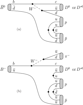
Typical quark-line diagrams for the three- and four-body modes with a
meson are shown in Fig. 1. The
three-body modes involve internal emissions of the boson,
whereas the four- and five-body modes involve internal and external
emission diagrams.
Figure 1:
Typical quark-line diagrams representing (a)
and (b)
modes.
The gluon lines are omitted.
The paper is organized as follows: Section II describes
the data sample and the BABAR detector. Section III
presents the analysis method, introducing the key variables and
. Section IV shows the fits to the joint
- distributions. The fit yields and the corresponding
branching fractions are given. Section V discusses the
systematic uncertainties. Section VI presents the
kinematic distributions. For the three-body modes, the Dalitz plots of
vs. are given as well as
the invariant mass plots of the variables. For the four- and
five-body modes, the two-body subsystem invariant mass plots are
given. In the four-body modes, we investigate a narrow structure in
the distribution near .
Section VII states the conclusions.
II BABAR DETECTOR AND DATA SAMPLE
We use a data sample with integrated luminosity of
( ) recorded at the
center-of-mass energy with the BABAR
detector at the PEP-II collider. The and beams
circulate in the storage rings at energies of and ,
respectively. The value of corresponds to the
mass, maximizing the cross section for
events. The production accounts for approximately a quarter
of the total hadronic cross section; the continuum processes
, , , and
constitute the rest.
The main components of the BABAR detector Aubert:2001tu are
the tracking system, the Detector of Internally-Reflected Cherenkov
radiation (DIRC), the electromagnetic calorimeter, and the
instrumented flux return.
The two-part charged particle tracking system measures the momentum.
The silicon vertex tracker, with five layers of double-sided silicon
micro-strips, is closest to the interaction point. The tracker is
followed by a wire drift chamber filled with a helium-isobutane
(:) gas mixture, which was chosen to minimize multiple
scattering. The superconducting coil creates a
solenoidal field.
The DIRC measures the opening angle of the Cherenkov light cone,
, produced by a charged particle traversing one of
the 144 radiator bars of fused silica. The light propagates in the
bar by total internal reflection and is projected onto an array of
photomultiplier tubes surrounding a water-filled box mounted at the
back end of the tracking system. The DIRC’s ability to distinguish
pions, kaons, and protons complements the energy loss measurements,
, in the tracking volume.
The calorimeter measures the energies and positions of electron-photon
showers with an array of 6580 finely-segmented Tl-doped CsI crystals.
The flux return is instrumented with a combination of resistive plate
chambers and limited streamer tubes for the detection of muons and
neutral hadrons.
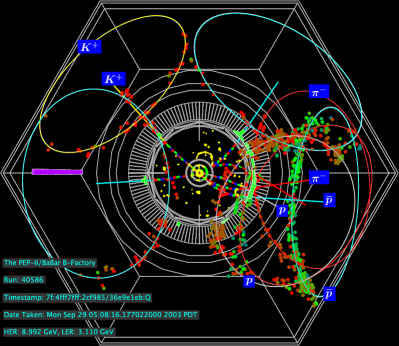
A data event display is given in Fig. 2 for the
candidate decay ,
.
Figure 2:
Event display for the candidate decay
,
. The labeled tracks in the
tracking system and DIRC rings at the perimeter correspond to the
particles in the reconstructed decay chain. The remaining
unlabeled tracks and rings are due to the decay of the other
meson in the event. The beam axis is perpendicular to
the image.
III ANALYSIS METHOD
This section describes the branching fraction measurement in four
parts. Section III.1 describes the Monte Carlo-simulated
event samples that are used to evaluate the performance of the method.
Section III.2 lists the discriminating variables and
their requirements for the event selection. Section III.3
defines the and variables and presents their
distributions for the newly observed modes. Lastly,
Sec. III.4 describes the fit to the -
distribution used to extract the signal yield.
III.1 Monte Carlo-simulated event samples
Monte Carlo (MC) event samples are produced and used to evaluate the
analysis method. Two types of samples—signal and generic—are
described below.
The particle decays are generated using a combination of
EvtgenLange:2001uf and Jetset 7.4Sjostrand:1993yb . The interactions of the decay products
traversing the detector are modeled by Geant 4Agostinelli:2002hh . The simulation takes into account varying
detector conditions and beam backgrounds during the data-taking
periods.
The signal MC sample is generated to characterize events with a
meson that decays to one of the signal modes (the accompanying
decays generically). The typical size of events per
decay chain is two orders of magnitude larger than the expected signal
in data.
The generic MC sample is generated to characterize the entire data
sample. The size is approximately twice that of the BABAR data
sample.
III.2 Event selection
The events are filtered for a signal -meson candidate
through the pre- and the final selections.
The pre-selection requires the presence of proton-antiproton pair and
a - or a -meson candidate (written as without a
charge designation) in one of the 26 decay chains listed in
Sec. I.
Protons are identified with a likelihood-based algorithm using the
and the measurements as
described in Sec II. For a proton in the lab
frame (typical of those produced in a signal mode), the selection
efficiency is and the kaon fake rate is .
The -meson candidates are selected using the invariant mass
fn:dmass , , and a kaon identification algorithm similar
to that used for protons. The is required to be within seven
times its resolution around the PDG value Amsler:2008zzb
(superseded later during final selection). For a kaon in
the lab frame (typical of those produced in a signal mode), the
selection efficiency is and the pion fake rate is .
For the and
sub-decay modes, the
candidates are formed from two
well-separated photons with or
from two unseparated photons by using the second moment of the
overlapping calorimeter energy deposits.
The charged particles from the decay chain are required to have a
distance of closest approach to the beam spot of less than cm.
The final selection requires the presence of a fully-reconstructed
signal -meson candidate. Requirements on the discriminating
variables described below are optimized by maximizing the signal
precision , where is the expected signal yield
using the signal MC sample and the expected background yield using
the generic MC sample. The signal is normalized using the measured
branching fractions for the modes
and
Anderson:2000tz ; Abe:2002tw ; for the rest of the modes the
latter value is used. The quantity is computed for each
discriminating variable for each decay chain. For the variables with
a broad maximum in , the cut values are chosen to be consistent
across similar modes.
In order to select -meson candidates, is required to be
within of the PDG value
Amsler:2008zzb . The resolutions for
, ,
, and
are approximately , ,
, and , respectively. For the modes involving
decays, the combinatoric
background events due to fake candidates are suppressed
using a model Frabetti:1994di that parameterizes the amplitude
of the Dalitz plot distribution
vs. . The model accounts for the amplitudes and
the interferences of decays of ,
, and
. The normalized magnitude of the
decay amplitude is used to suppress the background events by requiring
the quantity to be greater than a value ranging from to ,
depending on the mode.
In order to select -meson candidates, the -
mass difference, , is required to
be within of the PDG value
Amsler:2008zzb . The resolution is
approximately for both
and . For the mode
, the requirement
of excludes the contamination from
,
decays.
In order to select -meson candidates, a combination of daughter
particles in one of the signal modes is considered. The momentum
vectors of the decay products are fit Hulsbergen:2005pu while
constraining to the PDG value Amsler:2008zzb . The
vertex fit probability for non- events peaks sharply at
zero; these events are suppressed by requiring the probability to be
greater than .
Continuum backgrounds events are suppressed by using the angle
between the thrust axes Aubert:2001xs
of the particles from the -meson candidate and from the rest of the
event. The continuum event distribution of
peaks at unity while it is uniform for
events, so the quantity is required to be less than a value
ranging from to , depending on the mode.
After the selection, an average of to candidates per event
remains for each decay chain and is largest for those decay chains
with the largest particle multiplicity. If more than one candidate is
present, we choose the one with the smallest value of
(1)
where the PDG values Amsler:2008zzb are labeled as such. The
latter term in the sum is included only if a is present in
the decay chain. If more than one candidate has the same
value, we choose one randomly.
III.3 Definitions of and
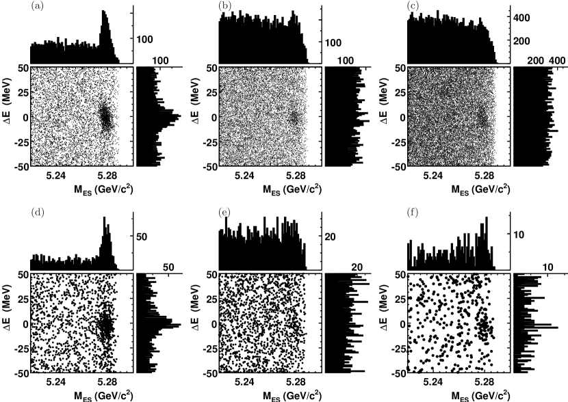
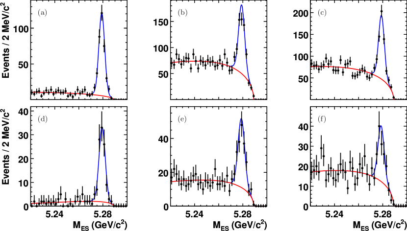
Figure 3:
Scatter plots of - for the six newly observed
-meson decay modes:
(a) ,
(b) ,
(c) ,
(d) ,
(e) ,
and (f) .
The first row of plots is related to the second by the exchange of
the charm meson . The decay chain
involving or
is shown. For (d, e, f),
the decay chain involves or
. The projection, in
bins, is given above the scatter plot; the , in
bins, on the right. For the projection plots, no selection
is made on the complementary variable.
The meson beam-energy-substituted mass, , and the difference
between its energy and the beam energy, , are defined with
the quantities in the lab frame:
(2)
The four-momentum vectors and
represent the -meson candidate and
the system, respectively. The two variables, when
expressed in terms of center-of-mass quantities (denoted by
asterisks), take the more familiar form,
and
.
The - distributions for the events passing the final
selection are given for the six newly observed modes in
Fig. 3. Each point represents a candidate in an event.
For many of the modes, a dense concentration of events is visible near
, the PDG -meson mass Amsler:2008zzb , and
, as expected for signal events. The uniform
distribution of events over the entire plane away from the signal area
is indicative of the general smoothness of the background event
distribution.
The - plots are given in a box region of
and . This box is
large enough to provide a sufficient sideband region for each variable
where no signal events reside. It is also small enough to exclude
possible contamination from other similarly related -meson decay
modes.
For the purpose of plotting and individually, the box
region is divided into a signal and a sideband region. The
signal region is within of the mean value of the
Gaussian function describing it and likewise for .
Similarly, the sideband region is outside of
the mean value and likewise for . The resolutions range from
to for and to for
. The signal box is the intersection of the
and the signal regions.
III.4 Fit procedure
The signal yield is obtained by fitting the joint -
distribution using a fit function in the
framework of the extended maximum likelihood technique
Barlow:1990vc . The likelihood value for observed events,
(3)
is a function of the yield estimate and the set of
parameters . The is the pair of and
values for the -meson candidate in the
event and is described below. The quantity is maximized
James:1975dr ; Verkerke ; Brun with respect to its arguments.
The fit function is the sum of two terms
(4)
which correspond to the signal and the background component,
respectively. For each component function, is the
two-dimensional function, the yield, and the
parameters. The arguments of the function components are related to the
quantities in Eq. (4) by
and .
Each function component is written as the product of
functions in and since the variables are largely
uncorrelated. (The signal bias due to the small correlation is
treated as a systematic uncertainty.) The distributions for signal
events peak in each variable, so is the product of
functions composed of a Gaussian core and a power-law tail
CBshape . The background event distribution varies smoothly, so
is the product of a threshold function
Aubert:2001xs for that vanishes at approximately
and a second-order Chebyshev polynomial for .
The following function parameters are fixed to the values found by
fitting the signal MC distributions: the Gaussian width for
, the Gaussian width for , the
power-law tail parameters for , and the
end-point parameter for . Two exceptions are given
after the detailed fit example.
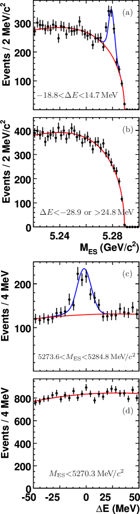
Figure 4:
Fit details for ,
: and
distributions in regions as noted on the plots. For (a, c) the
top curve is the sum of and and
the bottom curve is the latter; for (b, d) the curve is
.
A detailed example of the fit results is given in
Fig. 4 for the decay chain
,
. The plots in
Figs. 4a and 4b show the
distributions for the signal and the sideband
region, respectively. Likewise, Figs. 4c and
4d show the respective distributions for
the analogous regions. The fit function projections describe
the distributions in the sideband regions well
(Figs. 4b, 4d), which gives us
confidence that the background event distribution inside the signal
box are also modeled well.
The first exception to the fit procedure described above applies to
the mode . A term is
added to Eq. (4) to account for the sizable contamination
from the mode . The
fit function is the same form as
with its parameters fixed to the values found by fitting the MC
sample. The normalization is based on the branching
fraction measured in this paper.
The second exception applies to four decay chains whose fits do not
converge: ,
;
,
;
,
, ; and
,
,
. Two changes are made: the
Gaussian parameters are fixed to the values found in the
measurement, and the end-point
parameter is floated. The fits converge after the changes.
IV BRANCHING FRACTIONS
This section presents the -meson branching fractions .
Section IV.1 shows the fits to the -
distributions. Sections IV.2 and IV.3 gives
the values and their ratios, respectively. Throughout
this section, we simply state and use the systematic uncertainties of
Sec. V.
IV.1 Fits of -
distributions
The distributions for the events in the signal region
for three-, four-, and five-body modes are given in
Figs. 5–7, respectively. For all
-meson decay modes, the
decay chains involving or
show a peak.
The fit function projection in each plot describes the data well,
except for the four decay chains corresponding to
Figs. 7b, 7c, 7d,
and 7f, which had difficulties with fit convergence
as noted in the previous section. As we will see in
Sec. V, the yields from these decay chains do not
contribute significantly to the -meson branching fraction, which is
dominated by the value from , because
of their relatively large systematic uncertainties.
The signal yields, given in Table 1, range from
to events per mode.
Figure 5:
fit projections for the three-body modes:
(a–c) and
(d–f) ,
where
(a, d) are reconstructed via ,
(b, e) , and
(c, f) ; and
(d–f) .
Events with within of the mean value of
the Gaussian function are shown. The top curve is the sum
of and and the bottom curve
is the latter.
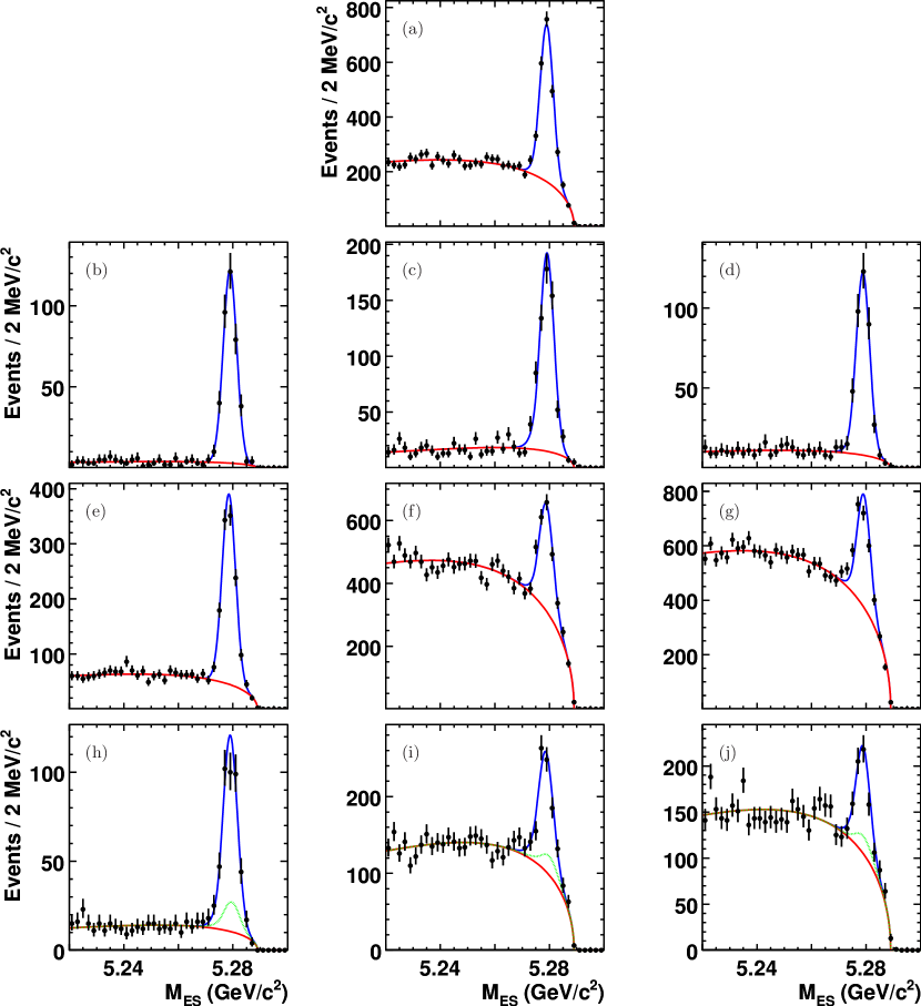
Figure 6:
fit projections for the four-body modes:
(a) ,
(b–d) ,
(e–g) , and
(h–j) ,
where
(a) is reconstructed via ,
(b, e, h) ,
(c, f, i) , and
(d, g, j) ; and
(b–d) and
(h–j) .
Events with within of the Gaussian mean
value are shown.
For (a–g) the top curve is the sum of
and and the bottom curve is the latter;
for (h–j) the middle curve is the sum of
and .
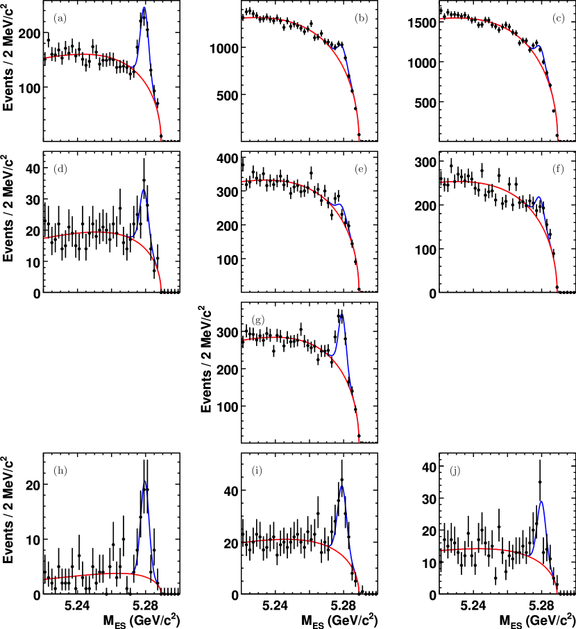
Figure 7:
fit projections for the five-body modes:
(a–c) ,
(d–f) ,
(g) , and
(h–j) ,
where
(a, d, h) are reconstructed via ,
(b, e, i) ,
(c, f, j) , and
(g) ; and
(b–d) and
(h–j) .
Events with within of the Gaussian mean
value are shown.
The top curve is the sum of and the
and the bottom curve is the latter. We
note that the plots in (b, c, e, f) had difficulties with fit
convergence; see text.
IV.2 Branching-fraction calculation
The -meson branching fraction for each of the twenty-six decay
chains, given in Table 1, is given by
(5)
whose ingredients are as follows: the number of pairs,
, the assumed
or
branching fraction, ; the -meson
branching fraction, Amsler:2008zzb ; the
-meson branching fraction,
Amsler:2008zzb ; the reconstruction efficiency, ; the
signal yield, ; and the measured contamination,
, using the -sideband data sample. The
is included only when a decay is
present in the decay chain. The efficiency is determined
using the signal MC sample and decreases with the particle
multiplicity. The mode ,
has the highest value of
at and
,
and
has the lowest at
.
The values, given in Table 2, are the
combinations Lyons:1988rp of the above measurements using the
statistical and the systematic uncertainties. All
values are significant with respect to their uncertainties. For the
previously observed modes, the results are consistent with earlier
measurements.
Table 1:
Intermediate values for Table 2: -meson
branching fractions for the decay chains. is
the yield, is the measured contamination
(item xvii in Table 4), and
is the reconstruction efficiency. The
uncertainties are statistical. The rows marked by a
dagger have large systematic uncertainties; see text.
The charges of the pions are implied as well as the
and
decays, when applicable.
modes, modes
(%)
()
,
,
,
,
,
,
,
,
,
,
,
,
,
,
,
,
,
,
,
,
,
,
,
,
,
,
Table 2:
Main results of this paper: -meson branching fractions for the
ten modes. Also given are the values of , the degrees of
freedom (DOF), and the probabilities for the averaging of
the results from Table 1. The measurements are
consistent with the previous results.
Table 3 gives the ratio of the branching fractions
for modes related by ,
, and the addition of
. These ratios show four patterns:
(i) The ratios are roughly unity for the modes related by the
spin of the charm mesons, . This result
suggests that the additional degrees of freedom due to the
polarization vector do not significantly modify the production rate.
(ii) The ratio is roughly unity for the modes related by the
charge of the charm mesons,
,
(iii) The ratio for the four-body mode to that of the corresponding
three-body mode with one fewer pion is about four.
(iv) The ratio for the five-body mode to that of the corresponding
four-body mode with one fewer pion is about one-half.
The patterns (iii, iv) imply
.
Table 3:
Ratios of -meson branching fractions of the modes related by
,
, and
the addition of . The uncertainties are statistical.
Ratio of the modes
Related by spin of charm meson
/
/
/
/
/
Related by charge of charm meson
/
/
/
/
Related by addition of pion to three-body modes
/
/
Related by addition of pion to four-body modes
/
/
/
/
V SYSTEMATIC UNCERTAINTIES
This section describes the systematic uncertainties for the -meson
branching fraction measurement. Section V.1 lists the
sources, and Sec. V.2 gives the error matrices.
V.1 Sources
The sources of systematic uncertainties, which are listed in
Table 4, can be organized as follows:
Table 4:
Systematic uncertainty list for -meson branching
fractions. The “ modes”
represents ,
, and ; and
.
Item
Description
Uncertainty ()
i
Number of pairs
ii
: for
iii
: for modes
, , ,
iv
: for ,
,
v
Charged particle reconstruction
vi
from
vii
reconstruction
viii
Signal mode decay dynamics
–
ix
Kaon and proton id using data
–
x
Kaon id in event topology
xi
Proton id in event topology
xii
Fit function params: for modes
, , ,
xiii
Signal fit function
xiv
Backgrnd. fit function: for modes
, , ,
xv
- correlation
–
xvi
Backgrnd. peaking in or for all modes (marked in Table 1)
– (–)
xvii
Backgrnd. from baryonic modes
–
(i) Counting of the number of pairs,
(ii–iv) Assumed branching fractions,
(v–xi) Reconstruction efficiencies,
(xii–xv) Fit functions and its parameters, and
(xvi–xvii) Backgrounds peaking in or .
These contributions are described below.
(i) The number of pairs used in the analysis is the
difference of the observed number of hadronic events and the expected
contribution from continuum events. The latter is estimated using a
separate data sample taken below the peak.
The uncertainty of is mostly due to the difference in the
detection efficiencies for hadronic events in the data and the MC
samples.
(ii) The branching fraction is assumed to be equal
for and . The uncertainty of is
the difference of and the PDG value Amsler:2008zzb .
(iii, iv) The - and -meson branching fractions
assume the PDG values Amsler:2008zzb . The
uncertainties of , , , and are the
PDG uncertainties for ,
, , and
, respectively; and and
for and
, respectively.
(v) The charged track reconstruction efficiency is evaluated using
events, where one tau decays
leptonically and the other hadronically. The uncertainty of
is due to the difference between the detection efficiency in the data
and the MC samples.
(vi) The reconstruction efficiency of low-energy charged pion from
decays is sufficiently
difficult, in comparison to other tracks, that item (v) cannot account
for its uncertainty. Such a pion is often found using only the
silicon vertex tracker because its momentum is relatively low. The
momentum dependence of pion identification is evaluated using the
helicity angle distribution—the angle between
the pion direction in the rest frame and the
boost direction—because the two quantities are highly
correlated. Since the pions are produced symmetrically in
, the observed asymmetry in the distribution
is indicative of the momentum dependence of the efficiency. The
uncertainty of is due to the difference in the momentum
dependence in the data and the MC samples.
(vii) The reconstruction efficiency is evaluated using
events as in item (v) with an uncertainty of .
(viii) The signal -candidate reconstruction efficiency is evaluated
using the MC samples. Since these samples use the uniform phase-space
decay model while the reported baryonic decay dynamics
(Lee:2004mg, ; Wang:2005fc, ; Medvedeva:2007zz, ; Wei:2007fg, ; Chen:2008jy, ; Aubert:2005gw, ; Anderson:2000tz, ; Abe:2002tw, ; Aubert:2006qx, , this paper)
are far from uniform, corrections are made in the variables where the
strongest variation are seen—in bins of
vs. —using the data and the MC samples.
The uncertainties ranging from to are due to the
limited statistics of the samples.
(ix) The particle identification efficiencies for kaons and protons
are evaluated using the MC samples, which are then corrected using a
data sample rich in these hadrons. The uncertainties ranging from
to are due to the sample statistics associated with the
correction procedure. The sample, however, is dominated by the
continuum events whose event topology is different from
events. Items (x, xi) account for the differences.
(x, xi) The kaon and proton identification efficiencies in the
environment are evaluated using a data sample of
,
and
decays, respectively. The uncertainties of and ,
respectively, are due to the differences in the event topologies.
(xii) A subset of the fit function parameters is fixed when fitting
the - distributions in the data sample. Such parameter
values are obtained by fitting the MC distributions, and they are
assigned an uncertainty from this fit. The effect on the signal yield
is evaluated by fitting the data sample with the parameter value
shifted by . The procedure is repeated for each parameter in
the set. The uncertainties of , , , and %
for the modes with ,
, ,
, and ,
respectively, are the quadrature sum of the fractional yield changes.
(xiii) The choice of the signal fit function is evaluated using an
alternate function, a fourth-order polynomial. The uncertainty of
is due to the yield difference with respect to the original
fit function.
(xiv) The choice of the background fit function is evaluated using a
more general fit function with the addition of another such component.
The uncertainties—, , , and for the
modes with , ,
, and
, respectively—are due to the
yield differences with respect to the original fit function.
(xv) The small correlation between the and
distributions introduces a bias in the signal yield. This effect is
quantified by fitting pseudo-experiments. Each experiment contains a
background sample whose and distributions are
produced according to , and a signal MC sample from
the full detector simulation. The uncertainties ranging from
to are from the deviation of to the mean of
the signal-yield distribution.
(xvi) Background events whose distributions peak either at
or can alter the signal yield.
For the measurement, the
variation of the normalization of the fit function for the
contribution within
the experimental uncertainties has a negligible effect on the signal
yield. For other decay modes, no such sources are found.
However, the distributions for a few cases feature a broad hump
with a width around spanning nearly half of the signal box.
The effect of the presence of such a source is quantified by adding a
component to the fit function whose parameters are
fixed except for the normalization. Except for four decay
chains—those corresponding to Figs. 7b,
7c, 7e, and
7f—uncertainties ranging from zero to are
obtained from the changes in yield when the additional component is
included. For the mentioned exceptions, the uncertainties range from
to . As a consequence of the large uncertainties, these
four modes do not contribute significantly to the final results.
(xvii) Background events from baryonic modes without a meson are
evaluated using the data sample. An example case where the final
states are identical is ,
and
,
. For such a source, the
distribution does not peak at the mass, so the
contamination can be quantified by repeating the analysis with the
-sideband region. is an additive correction
factor for with uncertainties ranging from to
due to the sample statistics.
V.2 Error matrices
Table 5:
Systematic uncertainties (%) combined for the modes. For
each mode, two columns are given. The uncorrelated values are
given on the left columns and the correlated on the right columns.
The right columns exclude items (iii, iv) of
Table 4.
unc
cor
unc
cor
00unc
cor00
unc
cor
-
-
-
-
-
-
-
-
-
-00
-
-
-
-
-
-
-
-
-
-
-
-
-
-
-
-00
-
-
The error matrix, , spanning the modes of a given
mode is the sum of the statistical and systematic components
.
The is the sum of a diagonal part and an
off-diagonal part
(Table 5). The is
diagonal with . The
is the sum of a diagonal part with
and an off-diagonal part with
. The correlation coefficient
is between two modes and .
The correlations among -meson branching fractions are the PDG
values Amsler:2008zzb ; all others are assumed to be unity.
VI KINEMATIC DISTRIBUTIONS
This section presents the kinematic distributions
BMassConstraint . Sections VI.1, VI.2,
and VI.3 give the plots for three-, four-, and five-body
modes, respectively. Additional discussion is devoted to the
feature in Sec. VI.4.
We briefly describe the background-subtraction and
efficiency-correction methods used to obtain the differential
branching fraction plots
(Figs. 9–11) as a function of
two-body invariant mass variables. The differential branching
fraction, in bins of the plotted variable, is the ratio of the
number of signal events and the product of the correction factors as
given in Eq. 5. The quantity in the numerator is the
sum of the background-subtracted event weights for events in bin ;
the formulae are given below. The efficiency-correction part of the
denominator is found for bin and is applied to each event weight.
The S-Plot method is used Pivk:2004ty to find the event weight,
(6)
where the is the pair of and values for the
candidate in the event; the fit functions
were defined in Eq. (4). In general, the weight is
approximately for a background event and for a signal event.
The quantifies the correlation between the
signal and the background yields,
(7)
VI.1 Three-body modes
For the three-body modes, plots are given for Dalitz variables and
two-body invariant masses.
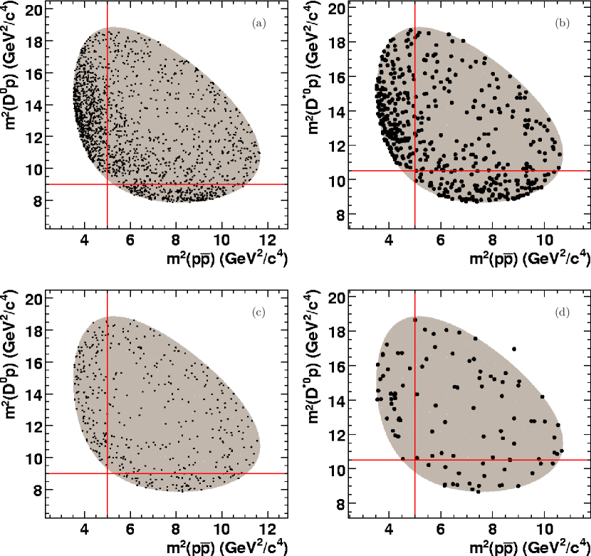
Figure 8:
Dalitz plots vs. for the
three-body modes. Plots in the first column (a, c) correspond to
; the second column (b, d)
. Plots in the first
row (a, b) are the events in the - signal box; the
second row (c, d) the events in the -sideband region
normalized to the amount of background present in the respective
plots in the first row. In the first row, near-threshold
enhancements are seen compared to the respective sideband plots in
the second row. The lines drawn at ,
, and are
visual aides to show that the enhancements are mostly
non-overlapping. The events are contained in the shaded contour
representing the allowed kinematic region except for one outlier
in (d), which failed the fit. The points are made larger for the
plots in the second column for better visibility.
The Dalitz plots of vs. for the
events in the - signal box are given
(Fig. 8a, 8b). The allowed kinematic
region is the shaded contour.
The background events present in Figs. 8a and
8b are represented by Figs. 8c and
8d, respectively. The latter plots show the events in
the -sideband regions with their normalizations determined from
the background yield in the signal box.
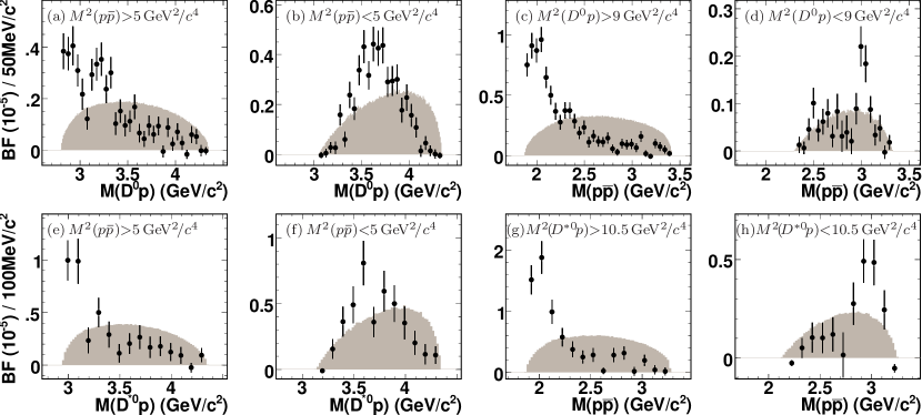
The two-body invariant mass plots are given in
Fig. 9. Differential branching fractions are
plotted as a function of and for
events in different regions of the complementary variable. The two
low-mass enhancements near threshold values in
and correspond to the dense regions in the Dalitz plots.
The broad enhancement in Fig. 9(d)
and 9(h) does not have a substantial contribution
from decays due to its width and current experimental limits
on
Aubert:2005tr .
In general, we observe a strong similarity between the shapes of the
corresponding distributions for
and
.
Figure 9:
Differential branching fraction plots for the three-body -meson
modes:
(a–d) and
(e–h) . The captions
give the various phase-space regions. The shaded region
represents the uniform phase-space model with its area normalized
to the data. The bin width for each row of plots is given on the
left-most plot.
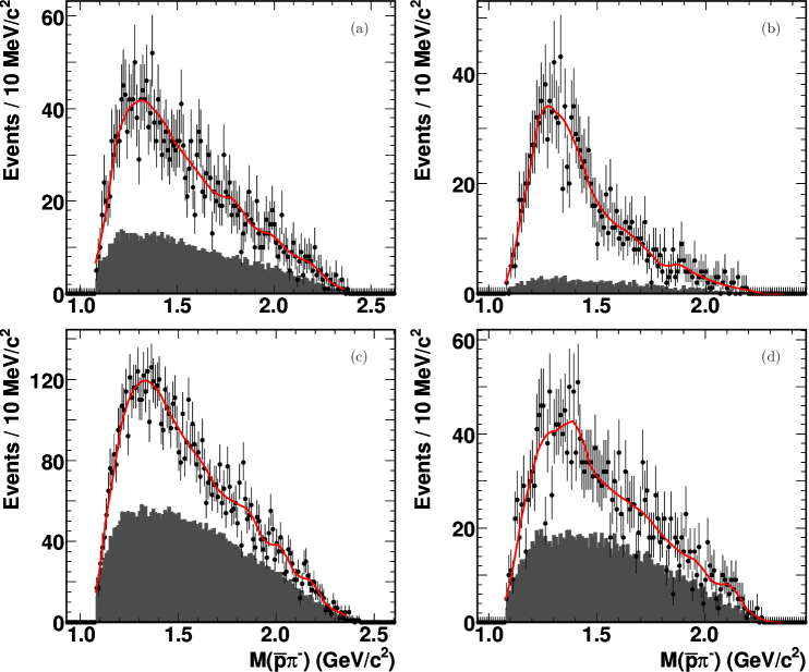
VI.2 Four-body modes
For the four-body modes, plots are given for two-body invariant masses
in Fig. 10. Differential branching fractions are
plotted as a function of , ,
, and .
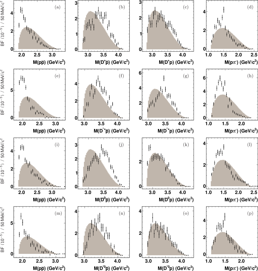
The two-body invariant-mass distributions show a number of features.
The distributions show a threshold enhancement with
respect to the expectations from the uniform phase-space decay model
(Figs. 10a, 10e,
10i, 10m). The
distributions show no indication of a
penta-quark resonance at Aktas:2004qf
(Figs. 10b, 10f,
10j, 10n). The
distribution in one of the modes
(Fig. 10k) suggests a threshold enhancement, as was
observed in the three-body modes, but the distributions in the other
modes show no such features (Figs. 10c,
10g, 10o). The
distribution in one of the modes (Fig. 10d) shows a
narrow structure near , but it is less prominent in the
distributions of the other modes (Figs. 10h,
10l, 10p).
The peak near does not correspond to a known state. The
peak is discussed in detail in Sec. VI.4.
Figure 10:
Differential branching fraction plots as
functions of , ,
, and for the
four-body -meson modes:
(a, b, c, d) ,
(e, f, g, h) ,
(i, j, k, l) , and
(m, n, o, p) ,
respectively. The shaded region represents the uniform
phase-space model normalized to the data. The possible presence
of a narrow peak near in plots in (d, h, j, p) are
shown in detail in Figs. 12a,
12b, 12c, and
12d, respectively, and discussed in
Sec. VI.4. The bin width for each row of plots is given on
the left.
VI.3 Five-body modes
For the five-body modes, plots are given for two-body invariant masses
in Fig. 11. Branching fractions are plotted as a
function of , ,
, and .
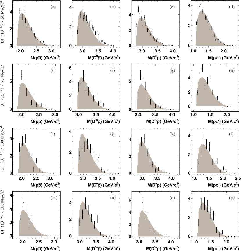
In contrast to the distributions for the three- and four-body modes,
the five-body distributions are generally more consistent with the
expectations from the uniform phase-space decay model.
A notable absence, again, is the signal of a penta-quark resonance at
Aktas:2004qf (Figs. 11b,
11f, 11j, 11n).
Figure 11:
Differential branching fraction plots as
functions of , ,
, and for five-body
-meson modes:
(a, b, c, d) ,
(e, f, g, h) ,
(i, j, k, l) , and
(m, n, o, p) ,
respectively. The shaded region represents the uniform
phase-space model normalized to the data. Each -meson
candidate for the plots in (d, h) contributes two entries for both
and combinations, so they are scaled
accordingly. The bin width for each row of plots is given on the
left.
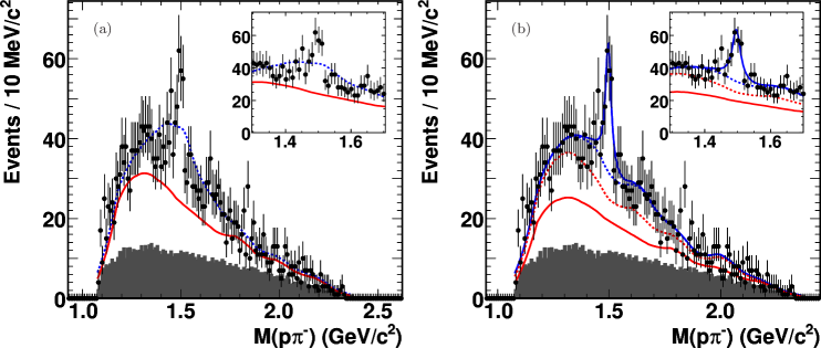
VI.4 Narrow peak at
The narrow peak in the fn:sign distribution at
, which we refer to as , is discussed in this section.
The opposite-sign distributions corresponding to
Figs. 10d, 10h,
10l, 10p are shown in more detail in
Fig. 12. In the detailed plots, the -axis bin
width is smaller at and the -axis is the
unweighted-uncorrected number of events. The events from the
-sideband region is superimposed with its normalization
determined from the background yield in the - signal
box.
In order to measure the properties of the peak, the fit formalism of
Eq. (4) is used. The signal component
is assumed to be a Breit-Wigner line shape. The background component
is taken from the same-sign
distribution. The distribution for the
mode is relatively smooth
(Fig. 13a), and it describes the rise and fall of
the opposite-sign distribution well (Fig. 12a),
whereas the same-sign distributions in the other modes show a more
rapidly falling behavior around
(Figs. 13b–13d).
We note, however, that the use of the shape for has
limitations. Since the formation of the or is not
necessarily symmetric with respect to the in these decays, the
same-sign combination may not predict the true shape
for the non-resonant component in the opposite-sign
distribution. As a consequence, we cannot precisely quantify the
systematic uncertainty associated with the lack of knowledge of the
true background shape.
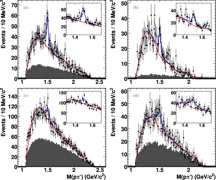
For the two neutral modes, the fits of the opposite-sign
distributions describe the entire kinematic range well
(Figs. 12a, 12b). We note a
small excess of events above with respect to
, but no peak component is included in the fit at
this mass. The fitted mass is and
, where the uncertainties are statistical, for
and
, respectively. We
measure the full widths to be and ,
respectively. The widths are significantly wider than detector
resolution, which is less than for a simulated
decay with a mass of and
negligible width.
In contrast to the neutral modes, the opposite-sign distributions
for the two charged modes exhibit a less peaking behavior at
. As a result, the parameter for the width in the
mode is fixed to the value
found in the mode; the
results of this fit are not used in the average.
The known nucleon resonances with the masses , ,
, and are used in an attempt to describe the .
The distribution is fit with the fit function components each
parameterized as a Breit-Wigner line shape. The normalization for each
component is allowed to vary independently. However, the fit does not
describe the peak because the is much narrower than any of the
resonances (Fig. 14a).
The overall significance of the is difficult to measure, due to
our lack of knowledge of the true background shape, as discussed
earlier, as well as further statistical issues. We caution that the
analysis is not blind, the parameters are not chosen a priori, and
the distribution under the no- hypothesis may be only approximately
normal. Furthermore, even under the normal assumption, the presence of
the mass and width nuisance parameters under the alternative
hypothesis means that the distributions of the statistic is not
likely to be pure .
We provide a measure of the statistical significance
of the in the two neutral
modes, where is the likelihood value with and
is without . The value is for
and for
.
The systematic uncertainties are mainly due to the .
We fit using an alternate fit function by adding a component derived
from the same-sign distribution of a different mode
(Fig. 14b). The result is a mass shift of
and a full width change of . An additional
contribution of is added for the mass measurement due to
the absolute uncertainty of the magnetic field and the amount of
detector material Aubert:2005gt .
In summary, the unknown structure can be characterized by a
Breit-Wigner line shape:
(8)
where the uncertainties are statistical and systematic, respectively.
Figure 12:
Fits of the opposite-sign distribution for
(a) ,
(b) ,
(c) , and
(d) for events
in the signal box of -. The top curve is the sum
of and while the bottom curve is
. The is from the corresponding
plot in Fig. 13. The shaded histograms are
scaled sidebands. A small inset plot is a close-up of the
region around ; its bin width is the same as in the
larger plot.
Figure 13:
Fits of the same-sign distribution for
(a) ,
(b) ,
(c) , and
(d) for events
in the signal box of -. The curve is the smoothed
histogram that is used in the corresponding plot in
Fig. 12 as . The shaded
histograms are scaled sidebands.
Figure 14:
Alternate fits of the opposite-sign distribution for
with
(a) various resonances and
(b) an additional obtained from the
sample.
The shaded histograms are the scaled - sidebands.
A small inset plot is a close-up of the region around ;
its bin width is the same as the larger plot.
VII CONCLUSIONS
We have presented a study of ten baryonic -meson decay modes of the
form using
a data sample of pairs. Significant
signals are observed (Table 1). Six of the
modes—,
,
,
,
, and
—are observed
for the first time (Figs. 6e–6g,
6h–6j, 7a,
7d, 7g,
7h–7j, respectively).
The -meson branching fraction measurements range from
to with the hierarchy
(Table 2). These results supersede the previous
BABAR publication of ,
, , and
Aubert:2006qx . The branching
fractions related by changes in the charge or the spin of the
meson are found to be similar (Table 3).
The kinematic distributions show a number of notable features. For
the three-body modes, threshold enhancements are present in
and (Figs. 8,
9). For the four-body modes, a threshold
enhancement is observed in and a narrow peak is seen in
(Fig. 10). For the five-body modes, in
contrast to the other modes, the distributions are similar to the
expectations from the uniform phase-space decay model
(Fig. 11).
The distributions in the neutral -meson decay mode
show the most prominent peak near . We obtained a mass of
and a full width of
, where the first uncertainties are statistical
and the second are systematic, respectively
(Figs. 12–14). Determining
the significance and interpreting the origin of the peak are
complicated by the fact that the background fit function is
parameterized by the distribution from the same-sign charge
combinations , a procedure which may not provide the
true background shape.
Despite the relatively small branching fractions for these modes of
order , with product branching fractions of order
to (including the and modes), the large size
of the BABAR data sample allowed us to observe signals containing
hundreds of events in many of the modes. We are, therefore, able to
probe their kinematic distributions that reflect the complex dynamics
of the multi-body final states.
VIII ACKNOWLEDGMENTS
We are grateful for the extraordinary contributions of our PEP-II
colleagues in achieving the excellent luminosity and machine
conditions that have made this work possible. The success of this
project also relies critically on the expertise and dedication of the
computing organizations that support BABAR. The collaborating
institutions wish to thank SLAC for its support and the kind
hospitality extended to them. This work is supported by the US
Department of Energy and National Science Foundation, the Natural
Sciences and Engineering Research Council (Canada), the Commissariat
à l’Energie Atomique and Institut National de Physique Nucléaire
et de Physique des Particules (France), the Bundesministerium für
Bildung und Forschung and Deutsche Forschungsgemeinschaft (Germany),
the Istituto Nazionale di Fisica Nucleare (Italy), the Foundation for
Fundamental Research on Matter (The Netherlands), the Research Council
of Norway, the Ministry of Education and Science of the Russian
Federation, Ministerio de Ciencia e Innovación (Spain), and the
Science and Technology Facilities Council (United Kingdom).
Individuals have received support from the Marie-Curie IEF program
(European Union), the A. P. Sloan Foundation (USA) and the Binational
Science Foundation (USA-Israel).
References
(1)
X. Fu et al. (CLEO Collaboration),
Phys. Rev. Lett. 79, 3125 (1997).
(2)
S. Anderson et al. (CLEO Collaboration),
Phys. Rev. Lett. 86, 2732 (2001).
(3)
I. Dunietz,
Phys. Rev. D 58, 094010 (1998).
(4)
B. Aubert et al. (BABAR Collaboration),
Phys. Rev. D 74, 051101 (2006).
(5)
K. Abe et al. (Belle Collaboration),
Phys. Rev. Lett. 89, 151802 (2002).
(6)
B. Aubert et al. (BABAR Collaboration),
Phys. Rev. D 78, 112003 (2008).
(7)
We do not include in
the list because they are beyond our sensitivity due to the
suppression with respect to
. For the quantity
, see
L. Wolfenstein, Phys. Rev. Lett. 51, 1945 (1983).
(8)
We use the convention that charge conjugation of particles and their
decays is implied unless otherwise specified.
(9)
Y. J. Lee et al. (Belle Collaboration),
Phys. Rev. Lett. 93, 211801 (2004).
(10)
M. Z. Wang et al. (Belle Collaboration),
Phys. Rev. D 76, 052004 (2007).
(11)
T. Medvedeva et al. (Belle Collaboration),
Phys. Rev. D 76, 051102 (2007).
(12)
J. T. Wei et al. (Belle Collaboration),
Phys. Lett. B 659, 80 (2008).
(13)
J. H. Chen et al. (Belle Collaboration),
Phys. Rev. Lett. 100, 251801 (2008).
(14)
B. Aubert et al. (BABAR Collaboration),
Phys. Rev. D 72, 051101 (2005) and
Ibid. 76, 092004 (2007).
(15)
W. S. Hou and A. Soni,
Phys. Rev. Lett. 86, 4247 (2001).
(16)
C. K. Chua, W. S. Hou, and S. Y. Tsai,
Phys. Rev. D 65, 034003 (2002);
Ibid. 66, 054004 (2002); and
Phys. Lett. B 544, 139 (2002).
(17)
H. Y. Cheng and K. C. Yang,
Phys. Rev. D 65, 054028 (2002)
(Erratum: Ibid. 65, 099901 (2002));
Ibid. 66, 014020 (2002);
Ibid. 66, 094009 (2002);
Ibid. 67, 034008 (2003);
Phys. Lett. B 533, 271 (2002); and
Ibid. 633, 533 (2006).
(18)
I. I. Bigi,
Eur. Phys. J. C 24, 271 (2002).
(19)
C. H. Chang and W. S. Hou,
Eur. Phys. J. C 23, 691 (2002).
(20)
H. Y. Cheng and K. C. Yang,
Phys. Rev. D 66, 014020 (2002);
Ibid. 65, 054028 (2002); and
Ibid. 67, 034008 (2003).
(21)
Z. Luo and J. L. Rosner,
Phys. Rev. D 67, 094017 (2003).
(22)
H. Y. Cheng,
J. Korean Phys. Soc. 45, S245 (2004);
Int. J. Mod. Phys. A 21, 4209 (2006); and
Nucl. Phys. Proc. Suppl. 163, 68 (2007).
(23)
Y. K. Hsiao,
Int. J. Mod. Phys. A 24, 3638 (2009).
(24)
M. Suzuki,
J. Phys. G 31, 755 (2005) and
Ibid. 34, 283 (2007).
(25)
T. M. Hong,
PhD thesis, Univ. of California, Santa Barbara,
SLAC Report 940, Works cited (2010) contains
a more comprehensive list of the literature.
(26)
J. L. Rosner,
Phys. Rev. Lett. 21, 950 (1968);
Phys. Rev. D 68, 014004 (2003);
Ibid. 69, 094014 (2004); and
private communications (2007).
(27)
A. Datta and P. J. O’Donnell,
Phys. Lett. B 567, 273 (2003).
(28)
B. Kerbikov, A. Stavinsky, and V. Fedotov,
Phys. Rev. C 69, 055205 (2004).
(29)
C. H. Chang and H. R. Pang,
Commun. Theor. Phys. 43, 275 (2005).
(30)
B. Aubert et al. (BABAR Collaboration),
Nucl. Instrum. Meth. A 479, 1 (2002).
(31)
D. J. Lange,
Nucl. Instrum. Meth. A 462, 152 (2001).
(32)
T. Sjostrand,
Comput. Phys. Commun. 82, 74 (1994).
(33)
S. Agostinelli et al. (Geant 4 Collaboration),
Nucl. Instrum. Meth. A 506, 250 (2003).
(34)
We follow the notation where is the invariant mass of the
reconstructed daughters of the -meson candidate.
(35)
C. Amsler et al. (Particle Data Group),
Phys. Lett. B 667, 1 (2008).
(36)
P. L. Frabetti et al. (E687 Collaboration),
Phys. Lett. B 331, 217 (1994).
(37)
W. D. Hulsbergen,
Nucl. Instrum. Meth. A 552, 566 (2005).
(38)
B. Aubert et al. (BABAR Collaboration),
Phys. Rev. D 65, 032001 (2002)
contains the definitions of the background fit function and
the thrust quantities.
(39)
R. J. Barlow,
Nucl. Instrum. Meth. A 297, 496 (1990).
(40)
F. James and M. Roos,
Comput. Phys. Commun. 10, 343 (1975).
(41)
W. Verkerke and D. Kirkby,
In Computing in High Energy and Nuclear Physics 2003
Conference Proceedings, La Jolla, California.
(42)
R. Brun and F. Rademakers,
Nucl. Instrum. Meth. A 389, 81 (1997).
(43)
M. J. Oreglia,
PhD thesis, Stanford Univ., SLAC Report 236, Appendix D (1980) and
J. E. Gaiser,
PhD thesis, Stanford Univ., Ibid. 255, Appendix F (1982).
(44)
L. Lyons, D. Gibaut, and P. Clifford,
Nucl. Instrum. Meth. A 270, 110 (1988).
(45)
For Sec. VI, we use a fit strategy where the decay
products’ momenta are fit while constraining the -meson
candidate’s to the PDG value Amsler:2008zzb . In
contrast, we do not impose this constraint for the
branching-fraction measurements. This strategy ensures that the
values of the kinematic variables for all the events lie within
the allowed limits.
(46)
M. Pivk and F. R. Le Diberder,
Nucl. Instrum. Meth. A 555, 356 (2005).
(47)
B. Aubert et al. (BABAR Collaboration),
Phys. Rev. D 71, 091103 (2005).
(48)
A. Aktas et al. (H1 Collaboration),
Phys. Lett. B 588, 17 (2004).
(49)
We refer to both and as opposite sign and to
both and as same sign.
(50)
B. Aubert et al. (BABAR Collaboration),
Phys. Rev. D 72, 052006 (2005).