Practical Top-K Document Retrieval in Reduced Space

Abstract

Supporting top-$k$ document retrieval queries on general text databases, that is, finding the $k$ documents where a given pattern occurs most frequently, has become a topic of interest with practical applications. While the problem has been solved in optimal time and linear space, the actual space usage is a serious concern. In this paper we study various reduced-space structures that support top-$k$ retrieval and propose new alternatives. Our experimental results show that our novel algorithms and data structures dominate almost all the space/time tradeoff.

1 Introduction

Ranked document retrieval is the basic task of most search engines. It consists in preprocessing a collection of $d$ documents, $\mathcal{D}=\{D_{1},D_{2},\ldots,D_{d}\}$, so that later, given a query pattern $P$ and a threshold $k$, one quickly finds the $k$ documents where $P$ is “most relevant”.

The best known application scenario is that of documents being formed by natural language texts, that is, sequences of words, and the query patterns being words, phrases (sequences of words), or sets of words or phrases. Several relevance measures are used, which attempt to establish the significance of the query in a given document [3]. The term frequency, that is, the number of times the pattern appears in the document, is the main component of most measures.

Ranked document retrieval is usually solved with some variant of a simple structure called an inverted index [27, 3]. This structure, which is behind most search engines, handles well natural language collections. However, the term “natural language” hides several assumptions that are key to the efficiency of that solution: the text must be easily tokenized into a sequence of words, there must not be too many different words, and queries must be whole words or phrases.

Those assumptions do not hold in various applications where document retrieval is of interest. The most obvious ones are documents written in Oriental languages such as Chinese or Korean, where it is not easy to split words automatically, and search engines treat the text as a sequence of symbols, so that queries can retrieve any substring of the text. Other applications simply do not have a concept of word, yet ranked retrieval would be of interest: DNA or protein sequence databases where one seeks the sequences where a short marker appears frequently, source code repositories where one looks for functions making heavy use of an expression or function call, MIDI sequence databases where one seeks for pieces where a given short passage is repeated, and so on.

These problems are modeled as a text collection where the documents $D_{i}$ are strings over an alphabet $\Sigma$, of size $\sigma$, and the queries are also simple strings. The most popular relevance measure is the plain term frequency, that is, the number of occurrences of the string $P$ in the strings $D_{i}$. We call $n=\sum|D_{i}|$ the collection size and $m=|P|$ the pattern length.

Muthukrishnan [20] pioneered the research on document retrieval for general strings. He solved the simpler problem of “document listing”: report the $occ$ distinct documents where $P$ appears in optimal time $O(m+occ)$ and linear space, $O(n)$ integers (or $O(n\log n)$ bits). Muthukrishnan also considered various other document retrieval problems, but not top-$k$ retrieval.

The first efficient solution for the top-$k$ retrieval problem was introduced by Hon, Shah, and Wu [15]. They achieved $O(m+\log n\log\log n+k)$ time, yet the space was superlinear, $O(n\log^{2}n)$ bits. Soon, Hon, Shah, and Vitter [14] achieved $O(m+k\log k)$ time and linear space, $O(n\log n)$ bits. Recently, Navarro and Nekrich [21] achieved optimal time, $O(m+k)$, and reduced the space from $O(n\log n)$ to $O(n(\log\sigma+\log d))$ bits (albeit the constant is not small).

While these solutions seem to close the problem, it turns out that the space required by $O(n\log n)$-bit solutions is way excessive for practical applications. A recent space-conscious implementation of Hon et al.’s index [23] showed that it requires at least 5 times the text size.

Motivated by this challenge, there has been a parallel research track on how to reduce the space of these solutions, while retaining efficient search time [24, 25, 14, 9, 7, 4, 22, 13]. In this work we introduce a new variant with relevant theoretical and practical properties, and show experimentally that it dominates previous work. The next section puts our contribution in context.

2 Related Work

Most of the data structures for general text searching, and in particular the classical ones for document retrieval [20, 14], build on on suffix arrays [18] and suffix trees [26, 1]. Regard the collection $\mathcal{D}$ as a single text $T[1,n]=D_{1}D_{2}\ldots D_{d}$, where each $D_{i}$ is terminated by a special symbol “$”. A suffix array $A[1,n]$ is a permutation of the values $[1,n]$ that points to all the suffixes of $T$: $A[i]$ points to the suffix $T[A[i],n]$. The suffixes are lexicographically sorted in $A$: $T[A[i],n]<T[A[i{+}1],n]$ for all $1\leq i<n$. Since the occurrences of any pattern $P$ in $T$ correspond to suffixes of $T$ that are prefixed by $P$, the occurrences are pointed from a contiguous area in the suffix array $A[sp,ep]$. A simple binary search finds $sp$ and $ep$ in $O(m\log n)$ time [18]. A suffix tree is a digital tree with $O(n)$ nodes where all the suffixes of $T$ are inserted and unary paths are compacted. Every internal node of the suffix tree corresponds to a repeated substring of $T$ and its associated suffix array interval;, suffix tree leaves correspond to the suffixes and their corresponding suffix array cells. A top-down traversal in the suffix tree finds the internal node (called the locus of $P$) from where all the suffixes prefixed with $P$ descend, in $O(m)$ time. Once $sp$ and $ep$ are known, the top-$k$ query finds the $k$ documents where most suffixes in $A[sp,ep]$ start.

A first step towards reducing the space in top-$k$ solutions is to compress the suffix array. Compressed suffix arrays (CSAs) simulate a suffix array within as little as $nH_{k}(T)+o(n\log\sigma)$ bits, for any $k\leq\alpha\log_{\sigma}n$ and any constant $0<\alpha<1$. Here $H_{k}(T)$ is the $k$-th order entropy of $T$ [19], a measure of its statistical compressibility. The CSA, using $|CSA|$ bits, finds $sp$ and $ep$ in time $\mathsf{search}(m)$, and computes any cell $A[i]$, and even $A^{-1}[i]$, in time $\mathsf{lookup}(n)$. For example, a CSA achieving the small space given above [8] achieves $\mathsf{search}(m)=O(m(1+\frac{\log\sigma}{\log\log n}))$ and $\mathsf{lookup}(n)=O(\log^{1+\epsilon}n)$ for any constant $\epsilon>0$. CSAs also replace the collection, as they can extract any substring of $T$.

In their very same foundational paper, Hon et al. [14] proposed an alternative succinct data structure to solve the top-$k$ problem. Building on a solution by Sadakane [24] for document listing, they use a CSA for $T$ and one smaller CSA for each document $D_{i}$, plus little extra data, for a total space of $2|CSA|+o(n)+d\log(n/d)+O(d)$ bits. They achieve time $O(\mathsf{search}(m)+k\log^{3+\epsilon}n\cdot\mathsf{lookup}(n))$, for any constant $\epsilon>0$. Gagie, Navarro, and Puglisi [9] slightly reduced the time to $O(\mathsf{search}(m)+k\log d\log(d/k)\log^{1+\epsilon}n\cdot\mathsf{lookup}(n))$, and Belazzougui and Navarro [4] further improved it to $O(\mathsf{search}(m)+k\log k\log(d/k)\log^{\epsilon}n\cdot\mathsf{lookup}(n))$.

The essence of the succinct solution by Hon et al. [14] is to preprocess top-$k$ answers for the lowest suffix tree nodes containing any range $A[i\cdot g,j\cdot g]$ for some sampling parameter $g$. Given the query interval $A[sp,ep]$, they find the highest preprocessed suffix tree node whose interval $[sp^{\prime},ep^{\prime}]$ is contained in $[sp,ep]$. They show that $sp^{\prime}-sp<g$ and $ep-ep^{\prime}<g$, and then the cost of correcting the precomputed answer using the extra occurrences at $A[sp,sp^{\prime}{-}1]$ and $A[ep^{\prime}{+}1,ep]$ is bounded. For each such extra occurrence $A[i]$, one finds out its document, computes the number of occurrences of $P$ within that document, and lets the document compete in the top-$k$ precomputed list. Hon et al. use the individual CSAs and other data structures to carry out this task. The subsequent improvements [9, 4] are due to small optimizations on this basic design.

Gagie et al. [9] also pointed out that in fact Hon et al.’s solution can run on any other data structure able to (1) telling which is the document corresponding to a given $A[i]$, and (2) counting how many times does the same document appear in any interval $A[sp,ep]$. A structure that is suitable for this task is the document array $D[1,n]$, where $D[i]$ is the document $A[i]$ belongs to [20]. While in Hon et al.’s solution this is computed from $A[i]$ using $d\log(n/d)+O(d)$ extra bits [24], we need more machinery for task (2). A good alternative was proposed by Mäkinen and Valimäki [25] in order to reduce the space of Muthukrishnan’s document listing solution [20]. The structure is a wavelet tree [12] on $D$. The wavelet tree represents $D$ using $n\log d+o(n)\log d$ bits and not only computes any $D[i]$ in $O(\log d)$ time, but it can also compute operation $rank_{i}(D,j)$, which is the number of occurrences of document $i$ in $D[1,j]$, within the same time. This solves operation (2) as $rank_{D[i]}(D,ep)-rank_{D[i]}(D,sp{-}1)$. With the obvious disadvantage of the considerable extra space to represent $D$, this solution changes $\mathsf{lookup}(n)$ by $\log d$ in the query time. Gagie et al. show many other combinations that solve (1) and (2). One of the fastest uses Golynski et al.’s representation [11] on $D$ and, within the same space, changes $\mathsf{lookup}(n)$ to $\log\log d$ in the time. Very recently, Hon, Shah, and Thankachan [13] presented new combinations in the line of Gagie et al., using also faster CSAs. The least space-consuming one requires $n\log d+n\,o(\log d)$ bits of extra space on top of the CSA of $T$, and improves the time to $O(\mathsf{search}(m)+k(\log k+(\log\log n)^{2+\epsilon}))$.

Belazzougui and Navarro [4] used an approach based on minimum perfect hash functions to replace the array $D$ by a weaker data structure that takes $O(n\log\log\log d)$ bits of space and supports the search in time $O(\mathsf{search}(m)+k\log k\log^{1+\epsilon}n\cdot\mathsf{lookup}(n))$. This is solution is intermediate between representing $D$ or the individual CSAs and it could have practical relevance.

Culpepper, Navarro, Puglisi, and Turpin [7] built on an improved document listing algorithm on wavelet trees [10] to achieve two top-$k$ algorithms, called Quantile and Greedy, that use the wavelet tree alone (i.e., without Hon et al.’s [14] extra structures). Despite their worst-case complexity being as bad as extracting one by one the results in $A[sp,ep]$, that is, $O((ep-sp+1)\log d)$, in practice the algorithms performed very well, being Greedy superior. They implemented Sadakane’s solution [24] of using individual CSAs for the documents and showed that the overheads are very high in practice. Navarro, Puglisi, and Valenzuela [22] arrived at the same conclusion, showing that Hon et al.’s original succinct scheme is not promising in practice: both space and time were much higher in practice than Culpepper et al.’s solution. However, their preliminary experiments [22] showed that Hon et al.’s scheme could compete when running on wavelet trees.

Navarro et al. [22] also presented the first implemented alternative to reduce the space of wavelet trees, by using Re-Pair compression [17] on the bitmaps. They showed that significant reductions in space were possible in exchange for an increase in the response time of Culpepper et al.’s Greedy algorithm (half the space and twice the time is a common figure).

This review exposes interesting contrasts between the theory and the practice in this area. On one hand, the structures that are in theory larger and faster (i.e., the $n\log d$-bits wavelet tree versus a second CSA of at most $n\log\sigma$ bits) are in practice smaller and faster. On the other hand, algorithms with no worst-case bound (Culpepper et al.’s [7]) perform very well in practice. Yet, the space of wavelet trees is still considerably large in practice (about twice the plain size of $T$ in several test collections [22]), especially if we realize that they represent totally redundant information that could be extracted from the CSA of $T$.

In this paper we study a new practical alternative. We use Hon et al.’s [14] succinct structure on top of a wavelet tree, but instead of brute force we use a variant of Culpepper et al.’s [7] method to find the extra candidate documents in $A[sp,sp^{\prime}{-}1]$ and $A[ep^{\prime}{+}1,ep]$. We can regard the combination as either method boosting the other. Culpepper et al. boost Hon et al.’s method, while retaining its good worst-case complexities, as they find the extra occurrences more cleverly than by enumerating them all. Hon et al. boost plain Culpepper et al.’s method by having precomputed a large part of the range, and thus ensuring that only small intervals have to be handled.

We consider the plain and the compressed wavelet tree representations, and the straightforward and novel representations of Hon et al.’s succinct structure. We compare these alternatives with the original Culpepper et al.’s method (on plain and compressed wavelet trees), to test the hypothesis that adding Hon et al.’s structure is worth the extra space. Similarly, we include in the comparison the basic Hon et al.’s method (with their structure compressed or not) over Golynski et al.’s [11] sequence representation, to test the hypothesis that using Culpepper et al.’s method over the wavelet tree is worth compared to the brute force method over the fastest sequence representation [11]. This brute force method is also at the core of the new proposal by Hon et al. [13].

Our experiments show that our new algorithms and data structures dominate almost all the space/time tradeoff for this problem, becoming a new practical reference point.

3 Implementing Hon et al.’s Succinct Structure

The succinct structure of Hon et al. [14] is a sparse generalized suffix tree of $T$ (SGST; “generalized” means it indexes $d$ strings). It is obtained by cutting $A[1,n]$ into blocks of length $g$ and sampling the first and last cell of each block (recall that cells of $A$ are leaves of the suffix tree). Then all the lowest common ancestors (lca) of pairs of sampled leaves are marked, and a tree $\tau_{k}$ is formed with those (at most) $2n/g$ marked internal nodes. The top-$k$ answer is stored for each marked node, using $O((n/g)k\log n)$ bits. This is done for $k=1,2,4,\ldots$, and parameter $g$ is of the form $g=k\cdot g^{\prime}$. The final space is $O((n/g^{\prime})\log d\log n)$ bits. This is made $o(n)$ by properly choosing $g^{\prime}$.

To answer top-$k$ queries, they search the CSA for $P$, to obtain the suffix range $A[sp,ep]$ of the pattern. Then they turn to the closest higher power of two of $k$, $k^{*}=2^{\lceil\log k\rceil}$, and let $g=k^{*}\cdot g^{\prime}$ be the corresponding $g$ value. They now find the locus of $P$ in the tree $\tau_{k^{*}}$ by descending from the root until finding the first node $v$ whose interval $[sp_{v},ep_{v}]$ is contained in $[sp,ep]$. They have at $v$ the top-$k$ candidates for $[sp_{v},ep_{v}]$ and have to correct the answer considering $[sp,sp_{v}{-}1]$ and $[ep_{v}{+}1,ep]$. Now we introduce two implementations of this idea.

3.1 Sparsified Generalized Suffix Tree (SGST)

Let us call $l_{i}=A[i]$ the $i$-th leaf. Given a value of $k$ we define $g=k\cdot g^{\prime}$, for a space/time tradeoff parameter $g^{\prime}$, and sample $n/g$ leaves $l_{1},l_{g+1},l_{2g+1},\ldots$, instead of sampling $2n/g$ leaves as in the theoretical proposal. We mark internal SGST nodes $lca(l_{1},l_{g+1}),lca(l_{g+1},l_{2g+1}),\ldots$. It is not hard to prove that any $v=lca(l_{ig+1},l_{jg+1})$ is also $v=lca(l_{rg+1},l_{(r+1)g+1})$ for some $r$ (more precisely, $r$ is the rightmost sampled leaf descending from the child of $v$ that is an ancestor of $l_{ig+1}$). Therefore these $n/g$ SGST nodes are sufficient and can be computed in linear time [5].

Now we note that there is a great deal of redundancy in the $\log d$ trees $\tau_{k}$, since the nodes of $\tau_{2k}$ are included in those of $\tau_{k}$, and the $2k$ candidates stored in the nodes of $\tau_{2k}$ contain those in the corresponding nodes of $\tau_{k}$. To factor out some of this redundancy we store only one tree $\tau$, whose nodes are the same of $\tau_{1}$, and record the class $c(v)$ of each node $v\in\tau$. This is $c(v)=\max\{k,~{}v\in\tau_{k}\}$ and can be stored in $\log\log d$ bits. Each node $v\in\tau$ stores the top-$c(v)$ candidates corresponding to its interval, using $c(v)\log d$ bits, and their frequencies, using $c(v)\log n$ bits, plus a pointer to the table, and the interval itself, $[sp_{v},ep_{v}]$, using $2\log n$ bits. All the information on intervals and candidates is factored in this way, saving space. Note that the class does not necessarily decrease monotonically in a root-to-leaf path of $\tau$, thus we store all the topologies independently to allow for efficient traversal of the $\tau_{k}$ trees, for $k>1$. Apart from topology information, each node of such $\tau_{k}$ trees contains just a pointer to the corresponding node in $\tau$, using $\log|\tau|$ bits.

In our first data structure, the topology of the trees $\tau$ and $\tau_{k}$ is represented using pointers of $\log|\tau|$ and $\log|\tau_{k}|$ bits, respectively. To answer top-$k$ queries, we find the range $A[sp,ep]$ using a CSA (whose space and negligible time will not be reported because it is orthogonal to all the data structures). Now we find the locus in the appropriate tree $\tau_{k^{*}}$ top-down, binary searching the intervals $[sp_{v},ep_{v}]$ of the children of the current node, and extracting those intervals using the pointer to $\tau$. By the properties of the sampling [14] it follows that we will traverse in this descent nodes $v\in\tau_{k^{*}}$ such that $[sp,ep]\subseteq[sp_{v},ep_{v}]$, until reaching a node $v$ so that $[sp_{v},ep_{v}]=[sp^{\prime},ep^{\prime}]\subseteq[sp,ep]\subseteq[sp^{\prime}-g,ep^{\prime}+g]$ (or reaching a leaf $u\in\tau_{k}$ such that $[sp,ep]\subseteq[sp_{u},ep_{u}]$, in which case $ep-sp+1<2g$). This $v$ is the locus of $P$ in $\tau_{k^{*}}$, and we find it in time $O(m\log\sigma)$. This time is negligible compared to the subsequent costs, as well as is the search using the CSA.

3.2 Succinct SGST

Our second implementation uses a pointerless representation of the tree topologies. Although the tree operations are slightly slower than on a pointer-based representation, this slowdown occurs on a not too significant part of the search process, and a succinct representation allows one to reduce the sampling parameter $g$ for the same space usage.

Arroyuelo et al. [2] showed that, for the functionality it provides, the most promising succinct representation of trees is the so-called Level-Order Unary Degree Sequence (LOUDS) [16]. It requires $2N+o(N)$ bits of space (in practice, as little as $2.1\,N$) to represent a tree of $N$ nodes, and it solves many operations in constant time (less than a microsecond in practice).

We use that implementation [2]. The shape of the tree is stored using a single binary sequence, as follows. Starting with an empty bitstring, every node is visited in level order starting from the root. Each node with $c$ children is encoded by writing its arity in unary, that is, $1^{c}0$ is appended to the bitstring. Each node is identified with the position in the bitstring where the encoding of the node begins. We store the values $sp_{v}$ and $ep_{v}$ in a separate array, indexed by the position of the node $v$ in the bitstring. Other node data such as pointers to $\tau$ (in $\tau_{k}$) and to the candidates (in $\tau$) are stored in the same way. The space can be further reduced by storing only the identifiers of the candidates, and their frequencies are computed on the fly using $rank$ on the wavelet tree of $D$.

4 A New Top-$k$ Algorithm

We run a combination of the algorithm by Hon et al. [14] and those of Culpepper et al. [7], over a wavelet tree representation of the document array $D[1,n]$. Culpepper et al. introduce, among others, a document listing method (DFS) and a Greedy top-$k$ heuristic. We adapt these to our particular top-$k$ subproblem.

If the search for the locus of $P$ ends at a leaf $u$ that still contains the interval $[sp,ep]$, Hon et al. simply scan $A[sp,ep]$ by brute force and accumulate frequencies. We use instead Culpepper et al.’s Greedy algorithm which is always better than a brute-force scanning.

When, instead, the locus of $P$ is a node $v$ where $[sp_{v},ep_{v}]=[sp^{\prime},ep^{\prime}]\subseteq[sp,ep]$, we start with the precomputed answer of the $k\leq k^{*}$ most frequent documents in $[sp^{\prime},ep^{\prime}]$, and update it to consider the subintervals $[sp,sp^{\prime}{-}1]$ and $[ep^{\prime}{+}1,ep]$. We use the wavelet tree of $D$ to solve the following problem: Given an interval $D[l,r]$, and two subintervals $[l_{1},r_{1}]$ and $[l_{2},r_{2}]$, enumerate all the distinct values in $[l_{1},r_{1}]\cup[l_{2},r_{2}]$ together with their frequencies in $[l,r]$. We propose two solutions, which can be seen as generalizations of heuristics proposed by Culpepper et al. [7].

4.1 Restricted Depth-First Search (DFS)

Figure 1 illustrates a wavelet tree representation of an array $D$ (ignore colors for now). At the root, a bitmap $B[1,n]$ stores $B[i]=0$ if $D[i]\leq d/2$ and $B[i]=1$ otherwise. The left child of the root is, recursively, a wavelet tree handling the subsequence of $D$ with values $D[i]\leq d/2$, and the right child handles the subsequence of values $D[i]>d/2$. Only the bitmaps $B$ are actually stored. Added over the $\log d$ levels, the wavelet tree requires $n\log d$ bits of space. With $o(n\log d)$ additional bits we answer in constant time any query $rank_{0/1}(B,i)$ over any bitmap $B$ [16].

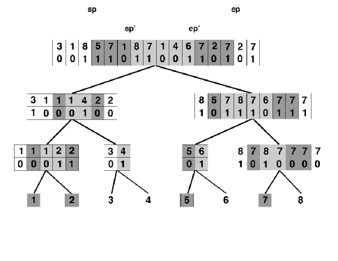
Figure 1: Restricted DFS to obtain the frequencies of documents not covered by $\tau_{k}$. Shaded regions show the interval $[sp,ep]=[4,14]$ mapped to each wavelet tree node. Dark shaded intervals are the projections of the leaves not covered by $[sp^{\prime},ep^{\prime}]=[7,11]$.

Note that any interval $D[i,j]$ can be projected into the left child of the root as $[i_{0},j_{0}]=[rank_{0}(B,i{-}1){+}1,rank_{0}(B,j)]$, and into its right child as $[i_{1},j_{1}]=[rank_{1}(B,i{-}1){+}1,rank_{1}(B,j)]$, where $B$ is the root bitmap. Those can then be projected recursively into other wavelet tree nodes.

Our restricted DFS algorithm begins at the root of the wavelet tree and tracks down the intervals $[l,r]=[sp,ep]$, $[l_{1},r_{1}]=[sp,sp^{\prime}{-}1]$, and $[l_{2},r_{2}]=[ep^{\prime}{+}1,ep]$. More precisely, we count the number of zeros and ones in $B$ in ranges $[l_{1},r_{1}]\cup[l_{2},r_{2}]$, as well as in $[l,r]$, using a constant number of rank operations on $B$. If there are any zeros in $[l_{1},r_{1}]\cup[l_{2},r_{2}]$, we map all the intervals into the left child of the node and proceed recursively from this node. Similarly, if there are any ones in $[l_{1},r_{1}]\cup[l_{2},r_{2}]$, we continue on the right child of the node. When we reach a wavelet tree leaf we report the corresponding document, and the frequency is the length of the interval $[l,r]$ at the leaf. Figure 1 shows an example where we arrive at the leaves of documents 1, 2, 5 and 7, reporting frequencies 2, 2, 1 and 4, respectively.

When solving the problem in the context of top-$k$ retrieval, we can prune some recursive calls. If, at some node, the size of the local interval $[l,r]$ is smaller than our current $k$th candidate to the answer, we stop exploring its subtree since it cannot contain competitive documents.

4.2 Restricted Greedy

Following the idea described by Culpepper et al., we can not only stop the traversal when $[l,r]$ is too small, but also prioritize the traversal of the nodes by their $[l,r]$ value.

We keep a priority queue where we store the wavelet tree nodes yet to process, and their intervals $[l,r]$, $[l_{1},r_{1}]$, and $[l_{2},r_{2}]$. The priority queue begins with one element, the root. Iteratively, we remove the element with highest $r{-}l{+}1$ value from the queue. If it is a leaf, we report it. Else, we project the intervals into its left and right children, and insert each such children containing nonempty intervals $[l_{1},r_{1}]$ or $[l_{2},r_{2}]$ into the queue. As soon as the $r{-}l{+}1$ value of the element we extract from the queue is not larger than the $k$th frequency known at the moment, we can stop.

4.3 Heaps for the $k$ Most Frequent Candidates

Our two algorithms solve the query assuming that we can easily know at each moment which is the $k$th best candidate known up to now. We use a min-heap data structure for this purpose. It is loaded with the top-$k$ precomputed candidates corresponding to the interval $[sp^{\prime},ep^{\prime}]$. At each point, the top of the heap gives the $k$th known frequency in constant time. Given that the previous algorithms stop when they reach a wavelet tree node where $r{-}l{+}1$ is not larger than the $k$th known frequency, it follows that each time the algorithms report a new candidate, this is more frequent than our $k$th known candidate. Thus we replace the top of our heap with the reported candidate and reorder the heap (which is always of size $k$, or less until we find $k$ distinct elements in $D[sp,ep]$). Therefore each candidate reported costs $O(\log d+\log k)$ time (there are also steps that do not yield any result, but the overall upper bound is still $O(g(\log d+\log k))$).

A remaining issue is that we can find again, in our DFS or Greedy traversal, a node that was in the original top-$k$ list, and thus possibly in the heap. This means that the document had been inserted with its frequency in $D[sp^{\prime},ep^{\prime}]$, but since it appears more times in $D[sp,ep]$, we must now update its frequency, that is, increase it and restore the min-heap invariant. It is not hard to maintain a hash table with forward and backward pointers to the heap so that we can track their current positions and replace their values. However, for the small $k$ values used in practice (say, tens or at most hundreds), it is more practical to scan the heap for each new candidate to insert than to maintain all those pointers upon all operations.

5 Experimental Results

We test the performance of our implementations of Hon et al.’s succinct structure combined with a wavelet tree (as explained, the original proposal is not competitive in practice [22]).

We used three test collections of different nature: ClueWiki is a 141 MB sample of ClueWeb09, formed by 3,334 Web pages from the English Wikipedia; KGS is a 75 MB collection of 18,838 sgf-formatted Go game records (http://www.u-go.net/gamerecords); and Proteins is a 60 MB collection of 143,244 sequences of Human and Mouse proteins (http://www.ebi.ac.uk/swissprot).

Our tests were run on a 4-core 8-processors Intel Xeon, 2Ghz each, with 16GB RAM and 2MB cache. We compiled using g++ with full optimization. For queries, we selected 1,000 substrings at random positions, of length 3 and 8, and retrieved the top-$k$ documents for each, for $k=1$ and $10$.

5.1 Choosing Our Best Variant

Our first round of experiments compares our different implementations of SGSTs (i.e., the trees $\tau_{k}$, see Section 3) over a single implementation of wavelet tree (Alpha, choosing the best value for $\alpha$ in each case [22]). We tested a pointer-based representation of the SGST (Ptrs, the original proposal [14]), a LOUDS-based representation (LOUDS), our variant of LOUDS that stores the topologies in a unique tree $\tau$ (LIGHT), and our variant of LIGHT that does not store frequencies of the top-$k$ candidates (XLIGHT). We consider sampling steps of 200 and 400 for $g^{\prime}$. For each value of $g$, we obtain a curve with various sampling steps for the $rank$ computations on the wavelet tree bitmaps.

We also tested different algorithms to find the top-$k$ among the precomputed candidates and remaining leaves (see Section 4): Our modified greedy (Greedy), our modified depth-first-search (DFS), and the brute-force selection procedure of the original proposal [14] on top of the same wavelet tree (Select). As this is orthogonal to the data structures used, we compare these algorithms only on top of the Ptrs structure. The other structures will use the best method.

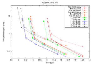
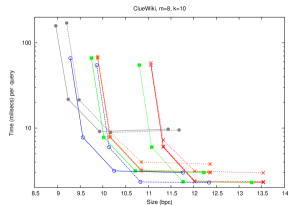
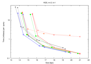
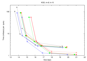
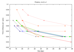
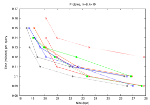
Figure 2: Our different alternatives for top-$k$ queries. On the left for $k=1$ and pattern length $m=3$; on the right for $k=10$ and $m=8$.

Figure 2 shows the results. Method Greedy is always better than Select (up to 80% better) and DFS (up to 50%), which confirms intuition. Using LOUDS representation instead of Ptr had almost no impact on the time. This is because time needed to find the locus is usually negligible compared with that to explore the uncovered leaves. Further costless space gains are obtained with variant LIGHT. Variant XLIGHT, instead, reduces the space of LIGHT at a noticeable cost in time that makes it not so interesting, except on Proteins. In various cases the sparser sampling dominates the denser one, whereas in others the latter makes the structure faster if sufficient space is spent.

To compare with other techniques, we will use variant LIGHT on ClueWiki and KGS, and XLIGHT on Proteins, both with $g^{\prime}=400$. This combination will be called generically SSGST.

5.2 Comparison with Previous Work

The second round of experiments compares ours with previous work. The Greedy heuristic [7] is run over different wavelet-tree representations of the document array: a plain one (WT-Plain) [7], a Re-Pair compressed one (WT-RP), and a hybrid that at each wavelet tree level chooses between plain, Re-Pair, or entropy-based compression of the bitmaps (WT-Alpha) [22]. We combine these with our best implementation of Hon et al.’s structure (suffixing the previous names with +SSGST). We also consider variant Goly+SSGST [9, 13], which runs the $rank$-based method (Select) on top of the fastest $rank$-capable sequence representation of the document array (Golynski et al.’s [11], which is faster than wavelet trees for $rank$ but does not support our more sophisticated algorithms; here we used the implementation at http://libcds.recoded.cl).

Our new structures dominate most of the space-time map. When using little space, variant WT-RP+SSGST dominates, being only ocassionally and slightly superseded by WT-RP. When using more space, WT-Alpha+SSGST takes over, and finally, with even more space, WT-Plain+SSGST becomes the best choice. Most of the exceptions arise in Proteins, which due to its incompressibility [22] makes WT-Plain+SSGST essentially the only interesting variant. The alternative Goly+SSGST is no case faster than a Greedy algorithm over plain wavelet trees (WT-Plain), and takes more space.

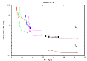
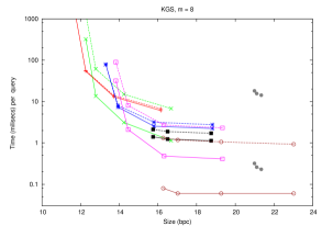
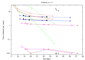
Figure 3: Comparison with previous work. On the left, for $m=3$, and on the right, for $m=8$.

6 Future Work

We can further reduce the space in exchange for possibly higher times. For example the sequence of all precomputed top-$k$ candidates can be Huffman-compressed, as there is much repetition in the sets and a zero-order compression would yield space reductions of up to 25% in the case of Proteins, the least compressible collection. The pointers to those tables could also be removed, by separating the tables by size, and computing the offset within each size using $rank$ on the sequence of classes of the nodes in $\tau$. Finally, values $[sp_{v},ep_{v}]$ can be stored as $[sp_{v},ep_{v}-sp_{v}]$, using DACs for the second components [6], as many such differences will be small.

References

- [1] A. Apostolico. The myriad virtues of subword trees. In Combinatorial Algorithms on Words, NATO ISI Series, pages 85–96. Springer-Verlag, 1985.
- [2] D. Arroyuelo, R. Cánovas, G. Navarro, and K. Sadakane. Succinct trees in practice. In Proc. 11th Workshop on Algorithm Engineering and Experiments (ALENEX), pages 84–97, 2010.
- [3] R. Baeza-Yates and B. Ribeiro-Neto. Modern Information Retrieval. Addison-Wesley, 2nd edition, 2011.
- [4] D. Belazzougui and G. Navarro. Improved compressed indexes for full-text document retrieval. In Proc. 18th International Symposium on String Processing and Information Retrieval (SPIRE), LNCS, 2011. To appear.
- [5] M. Bender and M. Farach-Colton. The LCA problem revisited. In Proc. 2nd Latin American Symposium on Theoretical Informatics (LATIN), pages 88–94, 2000.
- [6] N. Brisaboa, S. Ladra, and G. Navarro. Directly addressable variable-length codes. In Proc. 16th International Symposium on String Processing and Information Retrieval (SPIRE), LNCS 5721, pages 122–130, 2009.
- [7] J. S. Culpepper, G. Navarro, S. J. Puglisi, and A. Turpin. Top-k ranked document search in general text databases. In Proc. 18th Annual European Symposium on Algorithms (ESA), LNCS, pages 194–205 (part II), 2010.
- [8] P. Ferragina, G. Manzini, V. Mäkinen, and G. Navarro. Compressed representations of sequences and full-text indexes. ACM Transactions on Algorithms (TALG), 3(2):article 20, 2007.
- [9] T. Gagie, G. Navarro, and S. Puglisi. Colored range queries and document retrieval. In Proc. 17th International Symposium on String Processing and Information Retrieval (SPIRE), LNCS 6393, pages 67–81, 2010.
- [10] T. Gagie, S. J. Puglisi, and A. Turpin. Range quantile queries: Another virtue of wavelet trees. In Proc. 16th International Symposium on String Processing and Information Retrieval (SPIRE), LNCS 5721, pages 1–6, 2009.
- [11] A. Golynski, I. Munro, and S. Rao. Rank/select operations on large alphabets: a tool for text indexing. In Proc. 17th Annual ACM-SIAM Symposium on Discrete Algorithms (SODA), pages 368–373, 2006.
- [12] R. Grossi, A. Gupta, and J. S. Vitter. High-order entropy-compressed text indexes. In Proc. 14th ACM Symposium on Discrete Algorithms (SODA), pages 636–645, 2003.
- [13] W.-K. Hon, R. Shah, and S. Thankachan. Towards an optimal space-and-query-time index for top- document retrieval. CoRR, arXiv:1108.0554, 2011.
- [14] W.-K. Hon, R. Shah, and J. Vitter. Space-efficient framework for top- string retrieval problems. In 50th IEEE Annual Symposium on Foundations of Computer Science (FOCS), pages 713–722, 2009.
- [15] W.-K. Hon, R. Shah, and S.-B. Wu. Efficient index for retrieving top- most frequent documents. In Proc. 16th SPIRE, LNCS 5721, pages 182–193, 2009.
- [16] G. Jacobson. Space-efficient static trees and graphs. In Proc. 30th IEEE Symposium on Foundations of Computer Science (FOCS), pages 549–554, 1989.
- [17] J. Larsson and A. Moffat. Off-line dictionary-based compression. Proc. of the IEEE, 88(11):1722–1732, 2000.
- [18] U. Manber and G. Myers. Suffix arrays: a new method for on-line string searches. SIAM Journal on Computing, 22(5):935–948, 1993.
- [19] G. Manzini. An analysis of the Burrows-Wheeler transform. Journal of the ACM, 48(3):407–430, 2001.
- [20] S. Muthukrishnan. Efficient algorithms for document retrieval problems. In Proc. 13th Annual ACM-SIAM Symposium on Discrete Algorithms (SODA), pages 657–666, 2002.
- [21] G. Navarro and Y. Nekrich. Top- document retrieval in optimal time and linear space. In Proc. 22th Annual ACM-SIAM Symposium on Discrete Algorithms (SODA), 2012. To appear.
- [22] G. Navarro, S. Puglisi, and D. Valenzuela. Practical compressed document retrieval. In Proc. 10th International Symposium on Experimental Algorithms (SEA), LNCS 6630, pages 193–205, 2011.
- [23] M. Patil, S. Thankachan, R. Shah, W.-K. Hon, J. Vitter, and S. Chandrasekaran. Inverted indexes for phrases and strings. In Proc. 34th International ACM Conference on Research and Development in Information Retrieval (SIGIR), pages 555–564, 2011.
- [24] K. Sadakane. Succinct data structures for flexible text retrieval systems. Journal of Discrete Algorithms, 5(1):12–22, 2007.
- [25] N. Välimäki and V. Mäkinen. Space-efficient algorithms for document retrieval. In Proc. 18th Annual Symposium on Combinatorial Pattern Matching (CPM), LNCS 4580, pages 205–215, 2007.
- [26] P. Weiner. Linear pattern matching algorithm. In Proc. 14th Annual IEEE Symposium on Switching and Automata Theory, pages 1–11, 1973.
- [27] I. Witten, A. Moffat, and T. Bell. Managing Gigabytes. Morgan Kaufmann, 2nd edition, 1999.