The stellar metallicity distribution in intermediate latitude fields with BATC and SDSS data

Abstract

Based on the Beijing-Arizona-Taiwan-Connecticut (BATC) and Sloan Digital Sky Survey (SDSS) photometric data, we adopt SEDs fitting method to evaluate the metallicity distribution for $\sim$40, 000 main-sequence stars in the Galaxy. According to the derived photometric metallicities of these sample stars, we find that the metallicity distribution shift from metal-rich to metal-poor with the increase of distance from the Galactic center. The mean metallicity is about of $-1.5\pm 0.2$ dex in the outer halo and $-1.3\pm 0.1$ dex in the inner halo. The mean metallicity smoothly decreases from $-0.4$ to $-0.8$ in interval $0<r\leqslant 5$ kpc. The fluctuation in the mean metallicity with Galactic longitude can be found in interval $4<r\leqslant 8$ kpc. There is a vertical abundance gradients d[Fe/H]/dz $\sim-0.21\pm 0.05$ dex kpc^-1 for the thin disk ($z\leqslant 2$ kpc). At distance $2<z\leqslant 5$ kpc, where the thick disk stars are dominated, the gradients are about of $-0.16\pm 0.06$ dex kpc^-1, it can be interpreted as a mixture of stellar population with different mean metallicities at all $z$ levels. The vertical metallicity gradient is $-0.05\pm 0.04$ dex kpc^-1 for the halo ($z$ $>$ 5 kpc). So there is little or no metallicity gradient in the halo.

1 Introduction

The structure, formation and evolution of the Galaxy are very important issues in contemporary astrophysics. The basic components of Galaxy are the thin disk, the thick disk, the halo and central bulge, albeit that the inter-relationships and distinction among different components remain subject to some debate (Gilmore 1983; 1984; Lemon et al. 2004). Recent studies, based on accurate large-area surveys, have revealed that the Galaxy is marked by numerous irregular substructure such as the Sagittarius dwarf tidal stream in the halo (Ivezic et al. 2000; Yanny et al. 2000; Vivas et al. 2001; Majewski et al. 2003) and the Monoceros stream closer to the Galactic plane (Newberg et al. 2002; Rocha-Pinto et al. 2003). Carollo et al. (2007) shown that the the halo is clearly divisible into two broadly overlapping structural components - an inner and outer halo from a local kinematic analysis. It is now apparent that our Galaxy is much more complex system than we thought before. The formation of galaxies was long thought to be a steady process resulting in a smooth distribution of stars (Bahcall & Soneira 1981; Gilmore et al. 1989; Majewski 1993). But the view of the formation of the Galaxy has changed dramatically since the discoveries of complex substructures (Newberg et al. 2002; Belokurov et al. 2007). The presence of these lumpy and complex substructure are in qualitatively agreement with models for the formation of the stellar halo through the accretion and merging of nearby dwarf galaxies. Numerical simulations also suggest that this merger process plays a crucial role in setting the structure and motions of stars within galaxies (Bullock & Johnston 2005).

The abundance distribution is particular importance to understanding the formation and chemical evolution of the Galaxy (Freeman & Bland-Hawthorn 2002). Researchers have long sought to constrain models for the Galactic formation and evolution on the basis of observation of the stellar and clusters populations that it contains. Specific models of galaxy formation make specific predictions about the stellar abundance distribution. For example, stars on more radial orbits are more metal-poor than stars on planar orbits. This may indicate that the Milky Way formation began with a relatively rapid collapse of the initial proto-galactic cloud, which means the halo stars formed during the initial collapse, the disk stars formed after the gas had settled into the galactic plane. But the global collapse theory was unable to account for the lack of an abundance gradient in the Galactic halo (Searle & Zinn 1978). The current view is that the Galactic halo formed at least partly through the accretion of small satellite galaxies or merger of larger systems (Freeman et al., 2002), which is well-supported by studies of stellar kinematics and spatial distribution (Yannny et al. 2003; Juric et al. 2008). For the thick disk, it may be one of the most significant components for studying signatures of galaxy formation because it presents a snap frozen relic of the state of the early disk (Freeman 2002). An intrinsic abundance gradient in the thick disk would favor a scenarios which the thick disk was formed either in the slow late stages of the early Galactic collapse or the gradual kinematical diffusion of disk stars. On the contrary, a irregular metallicity distribution or absence of gradient would favor the thick disk having formed via the kinematical heating of thin disk or from merger debris (Siegel et al. 2009).

The metallicity distribution of the Galaxy is best probed directly through spectroscopic surveys (Yoss et al. 1987; Allende-Prieto et al. 2006). However, it has the advantage of using the photometric metallicity of many more stars out to limiting magnitude of photometric survey. Accurate determination of the properties of the Galactic components requires surveys with sufficient sky coverage to assess the overall geometry, sufficient depth for mapping stars to larger distance and sufficient information to obtain reasonable distance estimates for these stars (De Jong et al. 2010). Over the past few years, numerous surveys have been used to investigate the existence and size of the Galactic abundance gradient in the disk and halo. The existence of a radial gradient in the Galaxy is now well established. An average gradient of about $-0.06$ dex kpc^-1 is observed in the Galactic disk for most of the elements (Chen et al, 2003). De Jong et al. (2010) provided evidence for a radical metallicity gradients in the Galactic stellar halo. However, there is considerable disagreement about whether there is a vertical metallicity gradient among field and/or open cluster stars of the Galaxy.

The BATC multicolor photometric survey accumulated a large data base which is very useful for studying the Galactic structure and formation. Du et al. (2003) provided some information on the density distribution of the main components of the Galaxy, which can present constraints on the parameters of models of the Galactic structure. Later, they use F and G dwarfs from the BATC data to study the metal-abundance information (Du et al., 2004). With the new improved observation and improved knowledge regarding galaxy formation, it becomes possible to further discuss the metallicity gradient from different observation direction of the Galaxy.

In this paper, we attempt to study the metallicity gradient of the Milky Way galaxy using the 21 BATC photometric survey fields combined with the SDSS photometric data. The outlines of this paper is as follows: The BATC photometric system and data reduction are introduced briefly in Section 2. In Sect. 3 we describe the theoretical model atmospheric spectra and synthetic photometry. The metallicity distribution is discussed in Sect. 4. Finally in Sect. 5 we summarize our main conclusions in this study.

2 Observations and data

2.1 BATC photometric system and SDSS photometric system

The BATC survey performs photometric observations with a large field multi-colour system. There are 15 intermediate-band filters in the BATC filter system, which covers an optical wavelength range from 3000 to 10000 Å (Fan et al. 1996; Zhou et al. 2001). The 60/90 cm f/3 Schmidt Telescope of National Astronomical Observatories (NAOC) was used in the BATC program, with a Ford Aerospace 2048 $\times$ 2048 CCD camera at its main focus. The field of view of the CCD is $58^{\prime}$ $\times$ $58^{\prime}$ with a pixel scale of $1\arcsec{\mbox{}.}7$. The BATC magnitudes adopt the monochromatic AB magnitudes as defined by Oke & Gunn (1983). The PIPELINE II reduction procedure was performed on each single CCD frame to get the point spread function (PSF) magnitude of each point source (Zhou et al. 2003). The detailed description of the BATC photometric system and flux calibration of the standard stars can be found in Fan et al. (1996) and Zhou et al. (2001, 2003). In order to apply more color information to accurately estimate the photometric stellar metallicity, we combine the BATC colors with the SDSS colors message for the sample stars.

The SDSS used a dedicated 2.5 m telescope which has an imaging camera and a pair of spectrographs. The imaging camera (Gunn et al. 1998) contained 30 2048 $\times$ 2048 CCDs in the focal plane of the telescope. The flux densities of observed objects were measured almost simultaneously in five broad bands [ $u$, $g$, $r$, $i$, $z$] (Fukugita et al. 1996; Gunn et al. 1998; Hongg et al. 2001). For distinguishing explicitly between BATC and SDSS filter names, we refer to the SDSS filters and magnitudes as $u^{\prime}$, $g^{\prime}$, $r^{\prime}$, $i^{\prime}$, $z^{\prime}$. The photometric pipeline (Luption et al. 2001) detected the objects, matched the data from the five filters and measured instrumental fluxes, positions and shape parameters. The shape parameters allowed the classification of objects as point source or extended. The magnitudes derived from fitting a PSF are currently accurate to about 2 percents in $g$, $r$ and $i$, and 3-5 percents in $u$ and $z$ for bright ($\leq$ 20 mag) point source. In Table 1, we list the parameters of the BATC and SDSS filters. Col. (1) and Col. (2) represent the ID of the BATC and SDSS filters, Col. (3) and Col. (4) the central wavelengths and FWHM of the 20 filters, respectively. The reddening extinction for each star are determined from the SDSS catalog.

Table 1: Parameters of the BATC and SDSS filters

No.	Filter	Wavelength	FWHM
		(Å)	(Å)
1	$a$	3371.5	359
2	$b$	3906.9	291
3	$c$	4193.5	309
4	$d$	4540.0	332
5	$e$	4925.0	374
6	$f$	5266.8	344
7	$g$	5789.9	289
8	$h$	6073.9	308
9	$i$	6655.9	491
10	$j$	7057.4	238
11	$k$	7546.3	192
12	$m$	8023.2	255
13	$n$	8484.3	167
14	$o$	9182.2	247
15	$p$	9738.5	275
1	$u^{\prime}$	3543	569
2	$g^{\prime}$	4770	1387
3	$r^{\prime}$	6231	1373
4	$i^{\prime}$	7625	1526
5	$z^{\prime}$	9134	9500

2.2 Direction and data reduction

Accurate determination of the properties of components of the Milky Way requires surveys with sufficient sky coverage to assess the overall geometry (De Jong et al. 2010). Most previous investigations about the Galactic metallicity distribution use only one or a few selected lines-of-sight directions (Du et al. 2004; Siegel et al. 2009; Karatas et al. 2009). In this paper, the BATC photometry survey presented 21 intermediate-latitude fields in the multiple directions. These fields used in this paper are towards the Galactic center, the anticentre, the antirotation direction at median and high latitudes, $|b|>35^{\circ}$. Since metallicity distribution at high Galactic latitudes are not strongly related to the radial distribution, they are well suited to study the vertical distribution of the Galaxy. Table 2 lists the locations of the observed fields and their general characteristics. In Table 2, column 1 represents the BATC field name, columns 2 and 3 represent the Galactic longitude and latitude, columns 4 and 5 represent the limit magnitude and the number of sample star used in this study. As shown in the Table 2, the most photometric depth of our data is 21.0 mag in $i$ band. In total, there are about 40, 000 sample stars in our study.

Table 2: Relative information for the BATC observation fields

Observed field	$l$ (deg)	$b$ (deg)	$i$ (Comp)	star number
T485	175.7	37.8	21.0	1550
T518	238.9	39.8	19.5	1584
T288	189.0	37.5	20.0	2115
T477	175.7	39.2	20.0	2001
T328	160.3	41.9	19.5	1666
T349	224.1	35.3	20.5	2436
TA26	191.1	44.4	20.0	1285
T291	167.8	46.4	20.0	1670
T362	245.7	53.4	20.0	1237
T330	147.2	68.3	20.5	1020
U085	121.6	60.2	21.0	1679
T521	56.1	-36.8	20.5	4430
T491	62.9	-44.0	20.0	2824
T359	79.7	-37.8	20.5	2932
T350	251.3	67.3	19.5	1353
T534	91.6	51.1	21.0	2044
T193	59.8	-39.7	20.0	2830
T516	125.0	-62.0	20.0	1113
T329	169.9	50.4	21.0	1704
TA01	135.7	-62.1	20.5	1342
T517	188.6	-38.2	20.0	1296

Figure 1: Two-color diagrams for the BATC T329 field stars. The panel (a) is the distribution of sample stars in the ($j-m$)/($g-j$) two-colour diagram, and panel (b) is the ($j-m$)/($g-j$) two-colour diagram after removing those objects that lay significantly off the stellar locus. The line denotes the stellar locus from equation (1).

Here, because our fields in this work have also been observed by the Sloan Digital Space Survey (SDSS-DR7) and each object type (stars-galaxies-QSO) has been given. Thus, we can obtain a relative reliable star catalogue. In these star sample, it is complete to 20.5 mag with an error of less than 0.1 mag in the BATC $i$ band. Owing to the BATC observing strategy, data of stars brighter than $m$ = 14 mag, are saturated, and star counts are not completed for visual magnitudes fainter than $m$ = 21.0 mag. So our work is restricted to the magnitudes range 15 $\leqslant$ $i$ $<$ 21. From two-color diagrams for all objects in any field as an example, we can find that most stars are plotted on a diagonal band. In Fig. 1 show the BATC ($g-j$) versus ($j-m$) two-color diagram for T329 field stars. The line which can be described by equation (1) donates the stellar locus of the sample in the T329 field .

$$(j-m)=-0.10245+0.81172(g-j)$$ (1)

The sample shows a main-sequence (MS) stellar locus but has significant contamination from giants, manifested in the broader distribution overlying the narrow stellar locus. In order to determine the MS star sample, we use multi-color selection criteria outlined in Karaali et al. (2003) and Juric et al. (2008), which remove objects based on their location relative to the dominant stellar locus. For example, Juric et al. (2008) applied an extra procedure which consists of rejecting objects at distance larger than 0.3 mag from the stellar locus in order to remove hot dwarfs, low-red shift quasars, and white /red dwarf unresolved binaries from their sample. The procedure does well for high latitude field data from SDSS (Karaali et al. 2003; Yaz et al. 2010). Fig. 1b gives the cleaning sample stars after rejecting those objects which is lay significantly off the stellar locus.

3 THEORETICAL MODEL AND CALIBRATION FOR METALLICITY

3.1 theoretical stellar library and synthetic photometric

A homogeneous and complete stellar library can match any ambitious goals imposed on a standard library. Lejeune et al. (1997) presented a hybrid library of synthetic stellar spectra. The library covers a wide range of stellar parameters $T_{\rm eff}$= 50, 000 K to 2, 000 K in intervals of 250 K, log $g$= $-1.02$ to 5.50 in main increments of 0.5, and [M/H]= $-5.0$ to +1.0. For each model in the library, a flux spectrum is given for the same set of 1221 wavelength points covering the range 9.1 to 160, 000 nm, with a mean resolution of 20Å in the visible. The spectra are thus in a format which has proved to be adequate for synthetic photometry of wide- and intermediate-band systems (Du et al. 2004).

On the basis of the theoretical library, we calculate synthetic colors of the BATC and SDSS photometric system. Here, we synthesize colors for simulated stellar spectra with $T_{\rm eff}$ and log $g$ characteristic of main sequences (log $g$ = 3.5, 4.0, 4.5 for dwarfs) and 19 values of metallicity ([M/H]= $-5.0,-4.5,-4.0,-3.5$, $-3.0,-2.5,-2.0,-1.5,-1.0,-0.5$,$-0.3,-0.2,-0.1$, 0.0, +0.1, +0.2, +0.3, +0.5 and +1.0), where [M/H] denotes metallicity relative to hydrogen. The synthetic $i$th filter magnitude can be calculated with equation (2).

$$m=-2.5~{}{\rm log}\frac{\int{F_{\lambda}\phi_{i}({\lambda}){\rm d}\lambda}}{\int{\phi_{i}({\lambda}){\rm d}\lambda}}-48.60,$$ (2)

Where ${F_{\lambda}}$ is the flux per unit wavelength, $\phi_{i}$ is the transmission curve of the $i$th filter of the BATC or SDSS filter system (Du et al. 2004) .

The bluer colors are sensitive to metallicity down to the lowest observed metallicities because most of the line-blanketing from heavy elements occurs in the shorter wavelength regions. In contrast, the redder colors are primarily sensitive to temperature index. The BATC $a$, $b$ bands contain the Balmier jump, a stellar spectral feature which is sensitive to surface gravity. Since our sample includes only main sequences, it conveys little gravity information. It should be mentioned that, although the metallicity or temperature derived from synthetic photometry is not very accurate for a single star, perhaps which can be distorted by a poor point, it is meaningful for the statistic analysis of sample stars.

3.2 METALLICITY AND PHOTOMETRIC PARALLAX

The most accurate measurements of stellar metallicity are based on spectroscopic observation. Despite the recent progress in the availability of stellar spectra (e.g. SDSS-III and RAVE), the stellar number detected in photometric surveys is much more than spectroscopic observation. So photometric methods have also often been used to give the stellar metallicity. For example, Sandage (1969) detailed a technique using UBV photometry indices to measure approximate abundance. Karaali (2003) evaluated the metal abundance by ultraviolet-excess photometric parameter using CCD UBVI data. Karaali (2005) extended this method to the SDSS photometry. Ivezic et al. (2008) obtained the mean metallicity of stars as a function of $u-g$ and $g-r$ colors of SDSS data. For the BATC multicolor photometric system, there are 15 intermediate-band filters covering an optical wavelength range from 3000 to 10000 Å. There are 5 filters for the SDSS photometric system. So the SEDs of 20 filters for every object are equivalent to a low resolution spectrum.

The sample SEDs simulation with template SEDs can be used to derive the parameter of sample stars (Du et al. 2004). The standard minimization, computing and minimizing the deviations between the photometric SEDs of the star and the templates SEDs obtained with the same photometric system, is used in the fitting process. The minimum indicated the best fit to the observed SED by the set of spectra (Du et al. 2004).

$${\chi^{2}=\sum\limits_{l=1}^{N_{filt}=20}\left[\frac{m_{obs,l}-m_{temp,l}}{\sigma_{l}}\right]^{2}},$$ (3)

where ${m_{obs,l}}$, $m_{temp,l}$ and $\sigma_{l}$ are the observed magnitude, template magnitude and their uncertainty in filter $l$, respectively, and $N_{filt}$ is the total number of filters in the photometry.

According to the results of SEDs fitting, the metallicity and temperature of about 40, 000 sample stars are obtained in 21 fields. In addition, we extract the spectroscopic metallicities from sdss DR7 database for our studied 21 fields, and there are about 870 stars for which they also have photometric metallicities from our method. Using these stars, we present a calibration of our SED fitting method. After applying calibration, it is reliable for the derived photometric metallicities from SEDs fitting method. In Figure 2., we present the difference of photometric and spectroscopic metallicity as a function of $(g-r)$ color. The uncertainties of metallicity obtained from comparing SEDs between photometry and theoretical models are due to the observational error and the finite grid of the models. For the metal-poor stars ([Fe/H]$<-1.0$), the metallicity uncertainty is about 0.5 dex, and 0.2 dex for the stars [Fe/H]$>-0.5$ (Du et al. 2004). The metallicity distribution diagram for all sample stars was given in Fig. 3. One local maximum appear at [Fe/H] from -0.5 to 0 dex, and a tail down to -3.0 dex.

Figure 2: The difference of photometric and spectroscopic metallicity for 870 stars as a function of $(g-r)$ color is shown.

Figure 3: The metallicity distribution for all the sample stars selected in our study is shown.

The stellar type can be derived from effective temperature of dwarfs, then the stellar distance relative to the sun can be obtained by equation (4).

$$m_{v}-M_{v}=5lgr-5+A_{v}$$ (4)

where $m_{v}$ is the visual magnitude, absolute magnitude $M_{v}$ can be obtained according to the stellar type. The reddening extinction $A_{v}$ is small for most fields. We adopted the absolute magnitude versus stellar type relation for main-sequence stars from Lang (1992). $r$ is the stellar distances. The vertical distance of the star to the galactic plane can be evaluated by equation (5):

$$z=rsinb$$ (5)

A variety of errors affect the determination of stellar distances. The first source of errors is from photometric uncertainty less than 0.1 mag in the BATC $i$ band; the second from the misclassification, which should be small due to the multicolor photometry. For luminosity class V, types F/G, the absolute magnitude uncertainty is about 0.3 mag. In addition, there may exist an error from the contamination of binary stars in our sample. We neglect the effect of binary contamination on distance derivation due to the unknown but small influence from mass dsitribution in binary components (Kroupa et al. 1993; Ojha et al. 1996).

Figure 4: The metallicity distribution for the T291 field in different distance range is shown. In the short distance, r $<$ 1kpc, most stars are in the range [0, $-0.5$], in the larger distance, 15 $<$ r $<$ 20 kpc, most stars are poorer than $-1$.

4 METALLICITY DISTRIBUTION

It is well known that the chemical abundance of stellar population contains much information about the population^,s early evolution. The stellar metallicity distribution in the Galaxy has been the subject of photometric and spectroscopic surveys (Gilmore et al. 1985; Ratnatunga et al. 1989; Friel 1988). In this study, we want to explore possible stellar metallicity distribution variation with the observation direction. A method of SED combination for the SDSS and BATC photometries has been adopted to give the steller metallicity distribution. At first, the metallicity for the sample stars can be derived by comparing SEDs between photometry and the theoretical models. The SED fitting method is described in Section 3. 2. The mean metallicity distribution for each field is determined in the following distance intervals (in kpc): $15<r\leqslant 20$, $10<r\leqslant 15$, $8<r\leqslant 10$, $6<r\leqslant 8$, $5<r\leqslant 6$, $4<r\leqslant 5$, $3<r\leqslant 4$, $2.5<r\leqslant 3$, $2<r\leqslant 2.5$, $1.5<r\leqslant 2$, $1<r\leqslant 1.5$, $0.25<r\leqslant 1$. As an example the metallicity distributions as a function of vertical distance for the field T291 is presented in Fig. 4. From the figures (Fig.  4), it is clear that there is a number-shift from metal-rich stars to metal-poor ones with the increasing of distance. In star counts the younger metal rich stars are confined to regions close to the Galactic mid-plane, while the older, metal-poorer stars with a larger scale height dominated at larger vertical distances from the Galactic plane.

4.1 Metallicity variation with Galactic longitude

Mean metallicity distribution as a function of Galactic longitude for different distance intervals are presented in Fig. 5. The mean metallicity shift from metal-rich to metal-poor with the increase of distance from the Galactic center can be found in Fig. 5. The solid points represent the south galactic latitude fields, The open square points represent the north galactic latitude fields. As shown in Fig. 5, the mean metallicity in interval $10<r\leqslant 20$ kpc is around of $-1.5$ dex. In intervals $8<r\leqslant 10$ kpc our result indicates that the mean metallicity is $\sim$ $-1.3$. The mean metallicity in intervals $5<r\leqslant 8$ kpc is about $-1.0$ and the mean metallicity smoothly decreases from $-0.6$ to $-0.8$ in intervals $2.5<r\leqslant 5$ kpc. Our results are consistent with the results of Siegel et al. (2009) and Karatas et al. (2009). Siegel et al. find a monometallic thick disk and halo with abundances of [Fe/H] = $-0.8$ and $-1.4$ respectively. Karatas et al. derive mean abundance values of [Fe/H]= $-0.77\pm 0.36$ dex for the thick disk, and [Fe/H] = $-1.42\pm 0.98$. The mean metallicity decreases from $-0.4$ to $-0.6$ in intervals $0<r\leqslant 2.5$ kpc. The mean metallicity in interval $0.25<r\leqslant 1$ kpc is [Fe/H] $\sim$ $-0.3$, which is consistent with the result of Yaz et al. (2010).

As shown in Fig. 5, at larger distance, r $>$ 10 kpc, compared to the typical error bars, the mean metallicity distributions variation with Galactic longitude is almost flat. For $4<r\leqslant 8$ kpc, there is a fluctuation in the mean metallicity with Galactic longitude. The overall distribution of mean metallicity has a maxminum at $l$ $\sim$ 200^∘. For $2<r\leqslant 8$ kpc, the T517 filed (Galactic coordinates : $l=188.6^{\circ},b=-38.2^{\circ}$; Equatorial coordinates : $\alpha=58.59^{\circ}$, $\delta=-0.35^{\circ}$) and the TA26 field (Galactic coordinates : $l=191.1^{\circ},b=44.4^{\circ}$; Equatorial coordinates : $\alpha=139.956^{\circ}$, $\delta=33.745^{\circ}$) show metal rich character related to other fields. This feature may reflect a fluctuation from streams (such as Monocers stream) which are accreted from nearby galaxies. Juric et al.(2008) detect two overdensities in the thick disk region. Klement et al.(2009) also find individual stream from the SSPP in the direction with central coordinates (Equatorial coordinates): $\alpha$ = $58.58^{\circ}$ and $\delta$ = $-4.99^{\circ}$. Maybe the deviant behaviors of the two fields result from systematical error in the observation. In the work of AK et al. (2007), they find that the metallicity distributions for both (relatively) short and large vertical distances show systematic fluctuations. The scaleheight of thick disk varies with the observed direction were found in the works of Du et al. (2006) and Bilir et al. (2008).

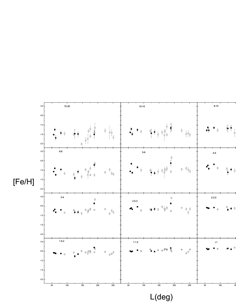
Figure 5: The mean metallicity distribution as a function of galactic longitude in different distance intervals are shown.

4.2 THE VERTICAL METALLICITY GRADIENT

Detailed information about the vertical metallicity gradient can provide important clue about the formation scenario of stellar population. Here, we used the mean metallicity to described the metallicity distribution function. As an example, The distribution trend of mean metallicity [Fe/H] with height above the galactic plane [$z$] for the T291 field is shown in Fig. 6. The metallicity gradients for all the fields in different $z$ intervals $z<2$ kpc, $2<z\leqslant 5$ kpc and $5<z\leqslant 15$ kpc are given in Fig. 7 and detailed in Table 3. In Table 3, Column 1 represents the BATC field name, Columns 2 - 7 represent gradient and error of gradient in different $z$ distance: $z\leqslant 2$ kpc, $2<z\leqslant 5$ kpc and $5<z\leqslant 15$ kpc, respectively.

From the Fig. 7 we can find that the variation of the gradient for the halo with galactic longitude is flat and the mean gradient of halo is about $-0.05\pm 0.04$ dex kpc^-1 ($5<z\leqslant 15$ kpc), which is essentially in agreement with the conclusion of Yaz et al. (2010) and Du et al. (2004). Du et al.(2004) find the small or zero gradient d[Fe/H]/dz = $-0.06\pm 0.09$ in the halo. Yaz et al. (2010) find $d[M/H]/dz=-0.01$ dex kpc^-1 for the inner spheroid. The result of Karaali et al. (2003) is slightly steeper than the value of our result. Karaali et al. (2003) find that there is a metallicity gradient d[Fe/H]/dz $\sim-0.1$ dex kpc^-1 in the inner halo ($5<z\leqslant 8$ kpc ) and zero in the outer part ($8<z\leqslant 10$ kpc). From Fig. 6 we can find that the incompleteness of the star sample causes significant statistical uncertainties at large distance. Probably, there is little or no metallicity gradient in the halo. It is consistent with the merger or accretion origin of the outer halo.

As shown in Fig. 7, at distance $0<z<2$ kpc, the mean vertical abundance gradient is about d[Fe/H]/dz $\sim-0.21\pm 0.05$ dex kpc^-1. The value for the vertical metallicity at distance $0<z<2$ kpc is in agreement with the canonical metallicity gradients with the same $z$ distances. For example, Yaz et al. (2009) find the metallicity gradient is d[Fe/H]/dz $\sim-0.3$ dex kpc^-1 for short distance. The metallicity gradient is found to be d[Fe/H]/dz $\sim-0.37$ dex kpc^-1 for $z$ $<$ 4 kpc in the work of Du et al. (2004). The result of Karaali et al. (2003) can be described as d[Fe/H]/dz $\sim-0.2$ dex kpc^-1 for the thin and thick disk.

At distance $2<z\leqslant 5$ kpc, where the thick disk stars dominated, the gradient is about $-0.16\pm 0.06$ dex kpc^-1 in our work which is consistent with the work of karaali et al. (2003) and less than the value of Du et al. (2004). Du et al. (2004) point out that the metallicity gradient is d[Fe/H]/dz $\sim$ $-0.37$ dex kpc^-1. In our study, the thick disk gradient is interpreted as different contribution from three components of the Galaxy at different $z$ distance. The existence of a clear vertical metallicity of the thick disk would be an important clue about the origin of the thick disk. However, it is an open question for the formation of the thick disk component. A number of models have been put forward since the confirmation if its existence. Chen et al. (2001) support that the thick disk formed through the heating of a preexisting thin disk, with the heating mechanism being the merging of a satellite galaxy. Here, we also favor the thick disk having formed via the kinematical heating of thin disk and from merger debris. Thus, there is a irregular metallicity distribution or absence of intrinsic gradient.

Figure 6: The mean metallicity as a function of vertical distance $z$ for the T291 field. The metallicity gradients of the thin disk, thick disk and halo are $-0.23\pm 0.03$, $-0.18\pm 0.07$, $-0.05\pm 0.01$ dex kpc^-1, respectively.

Figure 7: The metallicity gradients distribution for all fields in this study are shown for the intervals $z$ $<$ 2 kpc , 2 kpc $<$ $z$ $<$ 5kpc and 5 kpc $<$ $z$ $<$ 15kpc.

Table 3: The gradient distribution in different distance interval for the selected fields

	0-2 (kpc)		2-5 (kpc)		5-15 (kpc)
Observed field	gradient	error	gradient	error	gradient	error
T193	-0.136	0.017	-0.080	0.020	-0.020	0.022
T288	-0.258	0.027	-0.267	0.032	-0.007	0.037
T291	-0.228	0.028	-0.185	0.071	-0.045	0.014
T328	-0.110	0.027	-0.126	0.032	-0.137	0.043
T329	-0.170	0.028	-0.100	0.042	-0.037	0.015
T330	-0.171	0.042	-0.217	0.055	-0.080	0.010
T349	-0.180	0.017	-0.225	0.050	-0.029	0.031
T350	-0.267	0.033	-0.178	0.074	-0.069	0.035
T359	-0.203	0.017	-0.126	0.023	-0.054	0.023
T362	-0.237	0.037	-0.126	0.060	-0.037	0.022
T477	-0.181	0.025	-0.275	0.030	-0.053	0.022
T485	-0.247	0.033	-0.119	0.044	0.028	0.040
T491	-0.194	0.017	-0.179	0.020	-0.070	0.027
T516	-0.291	0.039	-0.204	0.061	-0.005	0.026
T517	0.054	0.041	-0.173	0.059	-0.101	0.067
T518	-0.163	0.035	-0.026	0.045	-0.051	0.052
T521	-0.197	0.012	-0.175	0.013	-0.045	0.011
T534	-0.254	0.028	-0.110	0.035	-0.035	0.012
TA01	-0.199	0.037	-0.192	0.046	-0.047	0.015
TA26	0.307	0.030	-0.187	0.038	-0.085	0.047
U085	-0.146	0.024	-0.148	0.037	-0.035	0.013

5 CONCLUSIONS AND SUMMARY

In this work, based on the BATC and SDSS photometric data, we evaluated the stellar metallicity distribution for 40, 000 main-sequence stars in the Galaxy by adopting SEDs fitting method. These selected fields are towards the Galactic center, the anticentre, the antirotation direction at median and high latitudes . The metallicity distribution could be obtained up to distances $r=20$ kpc, which covers the thin disk, thick disk and halo. We determined the mean stellar metallicity as a function of vertical distance in different direction. It can be clearly seen that the metallicity distribution shift from metal-rich to metal-poor with the increase of distance from the Galactic center. The mean metallicity is about $-1.5\pm 0.2$ dex in intervals $10<r\leqslant 20$ kpc and $-1.3\pm 0.1$ dex in interval $8<r\leqslant 10$ kpc. The mean metallicity smoothly decreases from $-0.6$ to $-0.8$ in interval $2.5<r\leqslant 5$ kpc, while the mean metallicity decreases from $-0.4$ to $-0.6$ in interval $0<r\leqslant 2.5$ kpc. In addition, a fluctuation in the mean metallicity with Galactic longitude can be found and the overall distribution has a maximum at about $l$ $\sim$ 200^∘ in interval $4<r\leqslant 8$ kpc. Maybe this feature can be related with the substructure or streams (such as Monoceros stream) which are accreted from nearby galaxies. At the same time, we find the vertical abundance gradients for the thin disk ($0<z<2$ kpc) is d[Fe/H]/dz $\sim-0.21\pm 0.05$ dex kpc^-1, and a vertical gradient $-0.16\pm 0.06$ dex kpc^-1 at distances $2<z\leqslant 5$ kpc where the thick disk stars are dominated. Here, we consider the thick disk gradient may be the result from the different contributions from three components of the Galaxy at different $z$ distance. The vertical gradient d[Fe/H]/dz $\sim-0.05\pm 0.04$ dex kpc^-1 is found in distance $5<z\leqslant 15$ kpc. So, there is little or no gradient in the halo. These results are in agreement with the values in the literature (Yoss et al. 1987; Trefzger et al. 1995; Karaali et al. 2003; AK et al. 2007; Yaz et al. 2010). It is possible that additional observational investigations (some projects aimed at spectroscopic sky surveys such as SEGUE, LAMOST, GAIA) will give more evidence for the metallicity gradient of the Galaxy and therefore provide a powerful clue to the disk and halo formation.

References

- Ak et al. (2007) AK S., Bilir S., Karaali S., Buser R., 2007, AN, 328, 169
- Ak et al. (2007) AK S., Bilir S., Karaali S., Buser R., Cabrera-Lavers A., 2007, NewA, 12, 605
- Allende et al. (2006) Allende Prieto C., Beers T. C., Wilhelm R., Newberg H. J., Rockosi C. M., Yanny B., Lee Y. S., 2006, ApJ, 636, 804
- Bahcall et al. (1981) Bahcall J. N., Soneira R. M., 1981, ApJS, 47, 357
- Belokurov et al. (2003) Belokurov V. A., Evans N. W. 2003, MNRAS, 341, 569
- Bilir et al. (2008) Bilir S., Cabrera - Lavers A., Karaali S., Ak S., Yaz E., López-Corredoira M., 2008, PASP, 25, 69
- Bullock et al. (2005) Bullock J. S., Johnston K. V., 2005, ApJ, 635, 931
- Du et al. (2003) C.-H. Du, et al. 2003, A&A, 407, 541
- Du et al. (2004) C.-H. Du, et al. 2004, AJ, 128, 2265
- Du et al. (2006) C.-H. Du, et al. 2006, MNRAS, 372, 1304
- Carollo et al. (2007) Carollo D., et al. 2007, Nature., 450, 1020
- Chen et al. (2001) Chen B. et al., 2001, ApJ, 553, 184
- Chen et al. (2003) Chen L., Hou J. L., Wang J. J., 2003, AJ, 125, 1397
- De et al. (2010) De Jong Jelte T. A.; Yanny B., Rix Hans-Walter, Dolphin A. E., Martin N. F., Beers T. C., 2010, ApJ, 714, 663
- Fan et al. (1996) Fan X. H. et al., 1996, AJ, 112, 628
- Freeman et al. (2002) Freeman K., Bland-Hawthorn J., 2002, ARA&A, 40, 487
- Friel (1988) Friel E. D., 1988, AJ, 95, 1727
- Fukugita et al. (1996) Fukugita M., Ichikawa T., Gunn J. E., Doi M., Shimasaku K., Schneider D. P., 1996, AJ, 111, 1748
- Gilmore et al. (1963) Gilmore G., Reid N., 1983, MNRAS, 202, 1025
- Gilmore (1984) Gilmore G., 1984, MNRAS, 207, 223
- Gilmore G & Wyse (1985) Gilmore G., Wyse R. F. G., 1985, AJ, 90, 2015
- Gilmore et al. (1989) Gilmore G., Wyse R. F. G., Kuijken K., 1989, ARA&A, 27, 555
- Gunn et al. (1998) Gunn J. E. et al., 1998, AJ, 116, 3040
- Hogg et al. (2001) Hogg D. W., Finkbeiner D. P., Schlegel D. J., Gunn J. E., 2001, AJ, 122, 2129
- Ivezic Z. et al. (2000) Ivezic Z. et al., 2000, AJ, 120, 963
- Ivezic Z. et al. (2008) Ivezic Z. et al., 2008, ApJ, 684, 287
- Juric et al. (2008) Juric M. et al., 2008, ApJ, 673, 864
- Karaali et al. (2003) Karaali S., AK S. G., Bilir S., Karatas Y., Gilmore G., 2003, MNRAS, 343, 1013
- Karaali et al. (2003) Karaali S., Bilir S., Karatas Y., Ak S. G., 2003, PASA, 20, 165
- Karaali et al. (2005) Karaali S., Bilir S., Tuncel S., 2005, PASA, 22, 24
- Karatas et al. (2009) Karatas Y., Kilic M., Günes O., Limboz F., 2009, PASP, 26, 1
- Klement et al. (2009) Klement R. et al., 2009, ApJ, 698, 865
- Kroupa et al. (1993) Kroupa P., Tout C. A., Gilmore G., 1993, MNRAS, 262, 545
- Lang et al. (1992) Lang K. R., 1992, Astrophysical Data I, Planets and Stars. Spinger-Verlag, Berlin
- Belokurov et al. (2003) Belokurov V. A., Evans N. W. 2003, MNRAS, 341, 569
- Lang et al. (1992) Lang K. R., 1992, Astrophysical Data I, Planets and Stars. Spinger-Verlag, Berlin
- Lejeune et al. (1997) Lejeune T., Cuisinier F., Buser R., 1997, A&AS, 125, 229
- Lemon et al. (2004) Lemon D. J., Wyse Rosemary F. G., Liske J., Driver S. P., Horne K., 2004, MNRAS, 347, 1043
- López -Corredoira et al. (2002) López -Corredoira M., Cabrera - Lavers A., Garzón F., Hammersley P. L., 2002, A&A, 394, 883
- Lupton et al. (2001) Lupton R. H., Gunn J. E., Ivezic Z., Knapp G. R., Kent S., 2001, ASPC, 238, 269
- Majewski et al. (2003) Majewski S. R., Skrutskie M. F., Weinberg M. D., Ostheimer J. C., 2003, ApJ, 599, 1082
- Majewski et al. (1993) Majewski S. R., 1993, ARA&A, 31, 575
- Newberg et al. (2002) Newberg H. J. et al., 2002, ApJ, 569, 245
- Ojha et al. (1996) Ojha D. K., Bienayme O., Robin A. C., Creze M., Mohan V., 1996, A&A, 311, 456
- Oke et al. (1983) Oke J. B., Gunn J. E., 1983, ApJ, 266, 713
- Ratnatunga et al. (1989) Ratnatunga K. U., Freeman K. C., 1989, ApJ, 339, 126
- Rocha-Pintoet al. (2003) Rocha-Pinto H. J., Majewski S. R., Skrutskie M. F., Crane J. D., 2003, ApJ, 594, 115
- Sandage et al. (1969) Sandage A., 1969, ApJ, 158, 1115
- Siegel et al. (2009) Siegel M. H., Karatas Y., Reid I. N., Yüksel R., I. Neill, 2009, MNRAS, 395, 1569
- Stetson (1987) Stetson P. B., 1987, PASP, 99, 191
- Searle et al. (1978) Searle L., Zinn R., 1978, ApJ, 225, 357
- Trefzger et al. (1995) Trefzger C. F., Pel J. W., Gabi S., 1995, A&A, 304, 381
- Vivas et al. (2001) Vivas A. K. et al., 2001, ApJ, 554, 33
- Xia et al. (2002) Xia L. F. et al., 2002, PASP, 114, 1349
- Yanny et al. (2000) Yanny B. et al., 2000, ApJ, 540, 825
- Yoss et al. (1987) Yoss K. M., Neese C. L., Hartkopf W. I., 1987, AJ, 94, 1600
- Yaz et al. (2010) Yaz E., Karaali S., 2010, NewA, 15, 234
- York et al. (2000) York D. et al., 2000, AJ, 120, 1579
- Zhou et al. (2003) Zhou X. et al., 2003, A&A, 397, 361