Dissipative electro-elastic network model of protein electrostatics

Abstract

ABSTRACT  We propose a dissipative electro-elastic network model (DENM) to describe the dynamics and statistics of electrostatic fluctuations at active sites of proteins. The model combines the harmonic network of residue beads with overdamped dynamics of the normal modes of the network characterized by two friction coefficients. The electrostatic component is introduced to the model through atomic charges of the protein force field. The overall effect of the electrostatic fluctuations of the network is recorded through the frequency-dependent response functions of the electrostatic potential and electric field at the active site. We also consider the dynamics of displacements of individual residues in the network and the dynamics of distances between pairs of residues. The model is tested against loss spectra of residue displacements and the electrostatic potential and electric field at the heme’s iron from all-atom molecular dynamics simulations of three hydrated globular proteins.

Key words: protein electrostatics; dissipative dynamics; elastic network; electrostatic response function; loss spectrum

INTRODUCTION

Proteins in solution exist not as static structures but instead as dynamic entities interconverting between conformational sub-states on the time-scale reflecting the activation barriers involved in the transitions (1, 2, 3). It is becoming increasingly clear that biomolecules are fluctuating machines, using dynamical equilibria between their conformational states to promote their function (2, 4). The flexibility of the protein structure naturally leads to changes in both the charge distribution of the protein itself and in the polarization of the interfacial waters following the protein motions. These dynamically fluctuating polarization fields will affect many properties sensitive to electrostatics, including the rates of enzymatic reactions (5). The dynamic nature of proteins, enhanced by the conformational manifold provided by hydration water (1), requires the shift of the focus from statistical averages and corresponding thermodynamic parameters, such as equilibrium Gibbs energies, to entire statistical distributions of observables and their dynamics expressed through time correlation functions.

This requirement is certainly the case for the problem of protein electron transfer, where, according to the standard Marcus picture (6), both the average of the energy gap between the donor and acceptor energy levels of the electron and its fluctuation are required to determine the probability of electron tunneling. This is just one example when the knowledge of the entire fluctuation spectrum of the observables is of significant interest (7). Other applications, such as electrostatic fluctuations reported by broad-band dielectric spectroscopy (8), THz absorption (9), and light scattering techniques (10) require either the entire fluctuation spectrum or a set of cumulants of the corresponding experimental observables.

With the general focus on the fluctuation spectrum of proteins, we propose here a model for the calculation of the statistics and dynamics of the electrostatic potential and electric field in proteins. Electrostatic interactions are clearly important for protein stability and function (5). Electrostatic solvation and interactions affect the stability of folded proteins and their aggregation and crystallization (11, 12, 13). Electrostatics might also play a significant role in promoting high-temperature flexibility of proteins through the coupling of the charge distribution in the protein to the electrostatic fluctuations produced by the protein-water interface (14).

The dynamics of electrostatic fluctuations spans an enormous range of time-scales from sub-picoseconds to sub-microseconds, and possibly longer (15, 16, 8). While spectroscopic techniques are capable of recording the ultra-fast fs-to-ps relaxation (17), the fluctuations of the protein-water interface recorded by Mössbauer spectroscopy and neutron scattering cover much longer time-scales from sub-nanoseconds to sub-microseconds (3). Our present model aims at these long, and perhaps even longer, time-scales by coarse-graining the protein into an elastic network of beads, each representing a protein residue.

Elastic network models have consistently shown good performance in characterizing global, large-scale motions of proteins (18, 19, 20, 21, 22, 23, 24, 25, 26, 27). While the low-frequency portion of the spectrum of protein motions is mostly determined by the distribution of mass and molecular shape (28, 29, 30), improvements are still needed to account for deficiencies of networks when localized protein motions are involved (31, 32, 33, 34). Electrostatic interactions, on the other hand, are notoriously long-ranged. The electrostatic potential, slowly changing over a nanometer-size biomolecule, effectively averages out local structural variations and is mostly sensitive to the global distribution of charge within the molecule. From this perspective, the combination of even a basic elastic network with the molecular charge distribution might be sufficient to describe the statistics of the potential fluctuations and their slow dynamics.

We propose here a model combining the distribution of molecular charge from the standard atomic force-fields with the dynamics and statistics of protein motions derived from an elastic network. To test the model, we employ all-atom Molecular Dynamics (MD) simulations of three hydrated heme proteins. Previous analysis of these data has emphasized the importance of nanosecond (ns) relaxation modes in the electrostatic fluctuations of the protein matrix and the protein-water interface (14, 35). This time-scale is relevant to biological function since heme proteins are typical components of biology’s energy chains transporting electrons on nanosecond-to-microsecond time-scales (36, 7). The nanosecond time-scale fluctuations are also consistent with the dynamics of the global motions of the network of residues. An elastic network model naturally fits the physics of the problem. The present contribution is a first step in developing network models of the electrostatic response of hydrated proteins. Here, we focus on the electrostatics of the protein matrix only, leaving the water component of the overall response to future studies.

THEORY AND METHODS

Elastic network model

A coarse-grained elastic network model (ENM) assigns a node to a collection of atoms reducing the computational burden of an all-atom normal-mode analysis. The typical coarse-graining is done on the level of individual aminoacids (1-bead model (37)). The position of the node is defined by the coordinates of the C^α atom. The springs connecting the nodes represent the bonded and non-bonded interactions within an accepted cutoff distance (18, 19, 20) or by a distance-dependent force constant (33, 38, 26, 39). The ENM diagonalizes the Hessian matrix $\mathbf{H}$ derived from a simplified Hookean potential suggested by Tirion (18). This potential, $E_{ij}=C(r_{ij}-r_{0,ij})^{2}/2$, describes the elongation $r_{ij}=|\mathbf{r}_{i}-\mathbf{r}_{j}|$ between nodes $i$ and $j$ in the network characterized by one universal force constant $C$ and the structural information stored in the equilibrium bead positions $\mathbf{r}_{0,i}$ ($r_{0,ij}=|\mathbf{r}_{0,i}-\mathbf{r}_{0,j}|$).

The Hessian $H_{ij}^{\alpha\beta}$ is a $3N\times 3N$ matrix representing the protein elastic energy as a quadratic form of the Cartesian displacements $\delta r_{i}^{\alpha}=r_{i}^{\alpha}-r_{0,i}^{\alpha}$ of individual beads in the network

$$E=(C/2)\sum_{i,j}H_{ij}^{\alpha\beta}\delta r_{i}^{\alpha}\delta r_{j}^{\beta}.$$ (1)

Here, $i$ and $j$ run between 1 and $N$, $\alpha,\beta$ indicate the Cartesian projections, and summation over repeated Greek indices is assumed here and throughout. The Hessian is diagonalized by the unitary matrix $\mathbf{U}$ producing $3N$ eigenvalues $\lambda_{m}$. This standard linear algebra formalism (18, 19) yields the statistical correlator between the displacements of residues $i$ and $j$ in the network

$$\langle\delta r_{i}^{\alpha}\delta r_{j}^{\epsilon}\rangle=(\beta C)^{-1}\sum_{m,\gamma}U_{mi}^{\gamma\alpha}\lambda_{m}^{-1}U_{mj}^{\gamma\epsilon},$$ (2)

where $\beta=1/(k_{\text{B}}T)$ is the inverse temperature.

If the network is characterized by a universal force constant and a cutoff, it yields a bell-shaped density of vibrational states. A refinement of that network by adopting a stronger coupling between covalently bound neighbors splits the density of states into two maxima, in better agreement with all-atom calculations (40, 24, 41). This approximation is adopted in our present calculations: the spring constant was multiplied by a constant factor $\varepsilon=100$ for covalent neighbors. In addition, a uniform cut-off radius of 15 Å was used in all calculations.

Overdamped network dynamics

The standard mechanical ENM outlined above obviously lacks dissipative dynamics. The equations of motion are harmonic, implying oscillatory time correlation functions. In contrast, most correlation functions of hydrated proteins observed by scattering (42, 8, 10) and relaxation (43) techniques are exponential, corresponding to the overdamped (Debye) dynamics, or stretched-exponential (8). Several approaches can be implemented to incorporate dissipative dynamics into the mechanical network of beads. Langevin equations of motion for the ENM potential, within the general framework of the Lamm-Szabo formalism (44), have been suggested (34, 48). This approach, and some early suggestions (45, 46), still requires parameterization (done by fitting the rotational and translational diffusion coefficients from MD) and, in addition, doubles the size of the matrix to be diagonalized. We have adopted here a more straightforward formalism not requiring additional computational resources.

Instead of a harmonically oscillating network, we have assumed for each normal mode $\mathbf{q}_{m}$, diagonalizing the network’s Hessian, an overdamped motion described by the dissipative memory kernel $\zeta(t)$ (47). The equation of motion for such overdamped dynamics is

$$\int_{0}^{t}\zeta(t-t^{\prime})\mathbf{\dot{q}}_{m}(t^{\prime})dt^{\prime}+\lambda_{m}\mathbf{q}_{m}=\mathbf{F}(t),$$ (3)

where $\mathbf{F}(t)$ is an external force.

The distinction between Eq. (3) and the Langevin network (34, 48) is worth emphasizing here. In the latter, uncoupled Langevin dissipative equations are first assigned to each bead of the network. However, it was noted that dissipative equations for the beads are likely to become coupled when the Langevin dynamics of beads are consistently derived by integrating out the fast degrees of freedom in the equations of motion (49). Given that the assignment of uncoupled Langevin equations to the individual beads is phenomenological from the onset, one can introduce similar phenomenology at a different level of the theory. Here, in the spirit of the standard normal-mode analysis, we introduce uncoupled dissipative equations for the normal modes (Eq. (3)). This is still a phenomenological assumption requiring further testing, but it reduces to the standard normal-mode analysis in the static limit.

When Laplace-Fourier transform (47) is applied to Eq. (3), the displacement response function for collective mode $\mathbf{q}_{m}$ follows

$$\chi_{m}(\omega)=\left[i\omega\tilde{\zeta}(\omega)+\lambda_{m}\right]^{-1},$$ (4)

where $\tilde{\zeta}(\omega)$ is the Laplace-Fourier transform of the friction kernel $\zeta(t)$. Extending this procedure to all normal modes of the network, one obtains the response function of bead displacements

$$\chi_{ij}^{\alpha\beta}(\omega)=C^{-1}\sum_{m}U_{mi}^{\gamma\alpha}\left[\lambda_{m}+i\omega\zeta(\omega)\right]^{-1}U_{mj}^{\gamma\beta}.$$ (5)

In this equation, the response function $\bm{\chi}_{ij}(\omega)$, which is a rank-2 tensor, represents the displacement of residue $i$ of the protein due to an oscillatory force with frequency $\omega$ applied to residue $j$ and propagated through the network to residue $i$. This response function is the basis of the dissipative electro-elastic network model (DENM) proposed here. At $\omega=0$, Eq. (5) returns the standard result of the ENM given by Eq. (2).

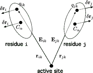
Figure 1: Cartoon illustrating the application of the dissipative electro-elastic network model (DENM) to the calculation of the electro-elastic response function at an atomic position in the active site of the protein. The elastic displacements of residues $i$ and $j$ create fluctuations of the electric fields by atomic charges $q_{ik}$ and $q_{jk}$. Electric fields $\mathbf{E}_{ik}$ and $\mathbf{E}_{jk}$ are produced by the corresponding charges $q_{ik}$ and $q_{jk}$ at the active site. The overall electric field of residue $i$ at the active site, $\mathbf{E}_{0i}$, is obtained by summation of all $\mathbf{E}_{ik}$ produced by the charges $q_{ik}$ of the residue.

Electrostatic potential response function

The ENM has shown good performance for low-frequency structural/mechanical deformations of individual proteins and biomolecular assemblies (27). Our goal here is to supplement these low-frequency motions with atomic partial charges to model the dynamics and statistics of electrostatic fluctuations at active sites of proteins. Coarse-grained electrostatics of proteins has been addressed in a number of recent papers (50, 51, 52), mostly dealing with long-range protein assembly and interactions (53). These approaches also involve coarse-graining of the charge distribution (51, 52) or generating effective charges to reproduce the protein’s external field (54). Given that we are interested in the electrostatic fluctuations, which are more sensitive to a local charge distribution, atomic charges from force-field potentials are more consistent with our purpose.

Our approach starts with solving the standard ENM problem to obtain a set of displacements $\delta\mathbf{r}_{im}$ for each normal mode $m$ with the eigenvalue $\lambda_{m}$. Each of these displacements is then applied to all charges $q_{ik}$ of residue $i$, where index $k$ runs over all atoms of residue $i$ (Fig. 1). Displacements $\delta\mathbf{r}_{im}$ in turn produce dipole moments $\delta\bm{\mu}_{ik}^{(m)}=q_{ik}\delta\mathbf{r}_{im}$ which interact with charges of the protein active site. The overall electrostatic effect of the fluctuating protein medium is given as a sum over all contributions from each partial charge of all the residues except for the active site. This cumulative effect of all protein charges is given by the frequency-dependent response function of the electrostatic potential $\chi_{\phi}(\omega)$

$$\chi_{\phi}(\omega)=-\sum_{i,j}E_{0j}^{\alpha}\chi_{ij}^{\alpha\beta}(\omega)E_{0i}^{\beta}.$$ (6)

Here, $E_{0i}^{\alpha}$ is the $\alpha$ Cartesian projection of the electrostatic field produced by all charges $q_{ik}$ of residue $i$ at an atom in the active site (Fig. 1)

$$E_{0i}^{\alpha}=-\sum_{k}\frac{q_{ik}(\mathbf{r}_{ik}-\mathbf{r}_{0})}{|\mathbf{r}_{ik}-\mathbf{r}_{0}|^{3}}.$$ (7)

Here, $\mathbf{r}_{0}$ is the position of the atom in the active site and $\mathbf{r}_{ik}$ is the position of charge $q_{ik}$ of residue $i$.

Electrostatic field response function

The potential response function $\chi_{\phi}(\omega)$ in Eq. (6) describes an oscillating electrostatic potential produced by the protein matrix in response to placing an oscillatory charge at the position in the active site where the potential is recorded (Fe ion in our MD simulations). Similarly, the response function of the electric field considers the field produced by the protein in response to an oscillating dipole moment $\mathbf{m}_{0}(t)=\mathbf{m}_{0}(\omega)\exp[i\omega t]$ placed in the active site. The deformation of the protein matrix induced by this probe dipole results in the electric field $\mathbf{E}_{0}(\omega)$ at the same site. It can be found by summation over the contributions from all individual dipoles $\delta\bm{\mu}_{ik}(\omega)$ arising from residues’ atomic charges

$$\mathbf{E}_{0}(\omega)=\sum_{ik}\mathbf{T}_{ik}\cdot\delta\bm{\mu}_{ik}(\omega).$$ (8)

Here, $\mathbf{T}_{ik}$ is the dipolar tensor connecting the position of the active site with the charge $q_{ik}$ of residue $i$. The dipole moment $\delta\bm{\mu}_{ik}(\omega)$ at the position of $q_{ik}$ is caused by the residue displacement $\delta\mathbf{r}_{ik}(\omega)$ and can be expressed in terms of the displacement response function

$$\delta\bm{\mu}_{ik}(\omega)=q_{ik}\sum_{j}\bm{\chi}_{ij}\cdot\delta\mathbf{F}_{j}(\omega),$$ (9)

where $\delta\mathbf{F}_{j}(\omega)=\sum_{k}q_{jk}\mathbf{T}_{jk}\cdot\mathbf{m}_{0}(\omega)$ is the force caused by the dipole $\mathbf{m}_{0}(\omega)$ at residue $j$. We therefore obtain a linear relation between the dipole $\mathbf{m}_{0}(\omega)$ placed at the active site and the electric field $\mathbf{E}_{0}(\omega)$ produced by the protein in response to this perturbation. The proportionality coefficient between the external perturbation and the response is the response function given by the rank-2 tensor

$$\chi_{E}^{\alpha\beta}(\omega)=\sum_{i,j,k,l}q_{ik}T_{ik}^{\alpha\gamma}\chi_{ij}^{\gamma\delta}(\omega)T_{jl}^{\delta\beta}q_{jl}.$$ (10)

Here, as above, the summation is done over the repeated Greek indices denoting the Cartesian components of the corresponding tensors. We will be mostly interested in the trace of the tensor

$$\chi_{E}(\omega)=\chi_{E}^{\alpha\alpha}(\omega).$$ (11)

Response and correlation functions

The response functions calculated by the DENM formalism need to be related to time correlation functions supplied by the MD trajectories. The dynamics of a general dynamical variable $\delta X(t)=X(t)-\langle X\rangle$ is characterized by the time self-correlation function

$$C_{X}(t)=\langle\delta X(t)\delta X(0)\rangle.$$ (12)

The normalized correlation function $S_{X}(t)=C_{X}(t)/\langle(\delta X)^{2}\rangle$ is related to the response function by the fluctuation-dissipation equation which forms the basis of our analysis (55)

$$\chi_{X}(z)=\beta\langle(\delta X)^{2}\rangle\left[1+iz\tilde{S}_{X}(z)\right],$$ (13)

where $\tilde{S}_{X}(z)$ is the Laplace-Fourier transform of $S(t)$ defined in the upper half of the complex plane of $z$.

Since our main focus is on variances of physical properties, we will define the generalized compliance for the variable $X$ as follows

$$\lambda_{X}=\beta\langle(\delta X)^{2}\rangle/2=\int_{0}^{\infty}\chi_{X}^{\prime\prime}(\omega)(d\omega/\pi\omega).$$ (14)

The same property can be calculated from the $\omega=0$ value of the real part of the response function

$$\lambda_{X}=(1/2)\chi_{X}^{\prime}(0).$$ (15)

In case of residue displacements considered as variable $X$ ($X=r$), $\lambda_{r}\propto C^{-1}$ is proportional to the inverse force constant of the network springs. As for the compliance of a macroscopic body, defined as the inverse of stiffness, $\lambda_{r}$ depends on the shape and boundary conditions, in contrast to elastic moduli representing material properties.

For the elastic network, the generalized compliance reports on how the softness of the network affects the variance of the variable of interest. In the case of $X=\phi$ reporting on the potential $\phi$ at the position of the heme’s iron, $\lambda=e^{2}\lambda_{\phi}$ is the reorganization energy of a half redox reaction corresponding to changing the oxidation state of the heme (6, 56). The standard definition of half-reaction reorganization energy involves, instead of one atom, the distribution of the electronic density of the transferred electron over a few atoms of the active site. We simplify this problem here by assuming all electron charge $e$ localized at the centroid of this charge density, the iron atom of the heme. The electrostatic potential at a single atom is a well defined physical property, but its variance is only an approximate representation of the observable reorganization energy of changing the redox state (6).

We want to gain insight into the dissipative dynamics of the elastic network and its comparison with the dynamics calculated from MD simulations. The loss function $\chi_{X}^{\prime\prime}(\omega)$ provides direct access to both the set of characteristic relaxation frequencies and their relative contributions. However, it does not weigh the low and high frequencies as they contribute to the variance in Eq. (14). Therefore, in addition to the loss function, we will consider the function

$$\alpha_{X}(\omega)=\frac{2}{\pi\omega}\ \frac{\chi_{X}^{\prime\prime}(\omega)}{\chi_{X}^{\prime}(0)}.$$ (16)

This function is normalized, $\int_{0}^{\infty}\alpha_{X}(\omega)d\omega=1$, and tends to the characteristic relaxation time $\langle\tau\rangle$ in the $\omega\to 0$ limit

$$\lim_{\omega\to 0}\alpha_{X}(\omega)=(2/\pi)\langle\tau\rangle,$$ (17)

where

$$\langle\tau\rangle=\int_{0}^{\infty}S_{X}(t)dt.$$ (18)

Proteins used in case studies and the simulation protocol

Three heme proteins, oxidized form of myoglobin (metmyoglobin, metMB, 1YMB) reduced state of cytochrome B562 (cytB, 256B), and reduced state of bovine heart cytochrome c (cytC, 2B4Z) were simulated by all-atom MD. The parameters of the proteins were taken from CHARMM27 force field (57), and NAMD (58) was used for the trajectories production. Each protein was placed at the center of a cubic box with the side length of $\simeq 108$ Å and solvated with TIP3P waters (59). The number of waters used in simulations were: 32891 (metMB), 33268 (cytB), and 33189 (cytC). The VMD (60) plugin Autoionize was used to neutralize the simulation cell by adding Na⁺ and Cl^- ions to bring the ionic strength of the solution to 0.1. Particle-mesh Ewald with the grid resolution $<1$ Å was used for electrostatic interactions, and all other non-bonded interactions were calculated within 12 Å cutoff. Following energy minimization, each protein was simulated for 5 ns in a NPT ensemble at $P=1$ atm and $T=300$ K. Temperature and pressure were controlled by using the Langevin dynamics with the damping coefficient of 5 ps^-1. The production NVE trajectory was started at the end of each 5 ns trajectory. The NVE ensemble is required for the proper sampling of the long-time dynamics since we found that using NPT and NVT ensembles artificially accelerates the observables relaxing on sub-nanosecond to nanosecond time-scale (61). The integration step was 2 fs and simulation frames for the analysis were saved each 0.05 ps. The simulation trajectories were 65 ns (metMB), 100 ns (cytC), and 123 ns (cytB).

The force field standard parameters of the heme in the reduced state are taken from CHARMM27 (57). The charge of iron is $q_{\text{Fe}}=0.24$ in the reduced state. No standard parameters are available for the oxidized heme required for the simulations of metmyoglobin. These force field parameters were taken from Autenrieth et al (62). The atomic charge of oxidized Fe is $q_{\text{Fe}}=1.34$ in this parametrization. The iron atom is five-coordinate in its oxidized state. In order to allow the iron to shift out of the porphyrin plane, the harmonic force constant of the bond between Fe and N${}_{\epsilon}2$ of histidine 93 was adjusted to 65 kcal/mol as suggested in Ref. (63) and also implemented in Ref. (64).

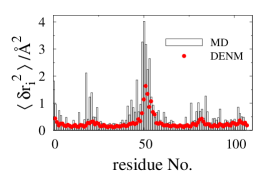
(a)

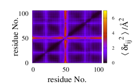
(b)

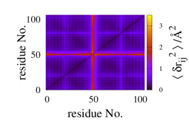
(c)

Figure 2: Residue mean-square displacements (msd’s) $\langle(\delta r_{i})^{2}\rangle$ (a) and variance-covariance matrix $\langle\delta\mathbf{r}_{i}\cdot\delta\mathbf{r}_{j}\rangle$ of residues’ $C^{\alpha}$ carbons calculated from MD (b) and from DENM (c). The diagonals in (b) and (c) represents the residue msd’s $\langle(\delta r_{i})^{2}\rangle$. The network force constant in the DENM calculations is $k_{\text{B}}T/C=1$ Ų. The DENM values indicated by red squares in (a) need to be multiplied by about a factor of two in order to obtain the best-fit agreement with the MD data. They are separated for a better visibility in the plot.

RESULTS AND DISCUSSION

Statistics and dynamics of residue displacements

Consistent with many previous studies, we have found that elastic networks are capable of reproducing the basic pattern of the distribution of mean-square displacements (msd’s) along the protein backbone. The left panel in Fig. 2 compares residue msd’s from MD with DENM calculations, while two other panels show the maps of variance-covariance matrices. Overall, there is a good agreement between the alteration in residue displacements along the backbone, and corresponding cross-correlations, calculated from the two sets of data. However, the network force constant required for the best fit of the msd from MD simulations, $\simeq 0.3$ kcal/(mol Ų), is somewhat lower than the value of $\simeq 1$ kcal/(mol Ų) typically adopted from fitting the B-factors from crystallography (18, 19, 20). This value is also about a factor of two lower than $0.6$ kcal/(mol Ų) adopted below to globally fit the variances of the field and electrostatic potential fluctuations from MD data for all three proteins studied here.

The fitting of the force constant to the absolute msd’s from MD makes the network too soft. This outcome is expected since the elastic network cuts high-frequency vibrations from the density of states and thus underestimates the absolute magnitudes of the residue displacements (27). It appears more consistent to use for the purpose of fitting only the portion of the msd related to protein’s global motions. This component can in fact be separated from the vibrational part in the temperature dependence of the msd since global motions of the protein become observable at high temperatures, above the temperature of the protein dynamical transition (65). This high-temperature portion of the protein msd is about a half of the total magnitude (66), which is close to the factor required to reconcile the force constants from electrostatic variances and msd’s.

Figure 3 shows the dynamics of positions $\mathbf{r}_{i}(t)$ of individual residues within the network and the dynamics of distances between residues $\mathbf{r}_{ij}(t)=\mathbf{r}_{i}(t)-\mathbf{r}_{j}(t)$. It reports the loss functions $\chi_{i}^{\prime\prime}(\omega)$ and $\chi_{ij}^{\prime\prime}(\omega)$ calculated from the self-correlation functions of individual residues

$$C_{i}(t)=\langle\delta\mathbf{r}_{i}(t)\cdot\delta\mathbf{r}_{i}(0)\rangle$$ (19)

and self-correlation functions of distances between the residues

$$C_{ij}(t)=\langle\delta\mathbf{r}_{ij}(t)\cdot\mathbf{r}_{ij}(0)\rangle.$$ (20)

These latter correlation functions are experimentally available from FRET (67) recording the evolution of the distance between two residues tagged with chromophores.

The comparison of $\chi_{i}^{\prime\prime}(\omega)$ from DENM and MD is illustrated in Fig. 3a for only one residue, $i=21$, belonging to cytB protein. The pair of residues with $i=21$ and $j=84$ is used to calculate $C_{ij}(t)$ in Fig. 3b. The position of the pair in the backbone of cytB is shown in Fig. 4. Examples of calculations for several additional pairs of residues from cytB can be found in Supporting Materials.

Both correlation functions, $C_{i}(t)$ and $C_{ij}(t)$, report the dynamics on roughly two time-scales, seen as two peaks in the their loss functions in Fig. 3. The two peaks represent, with varying weights, the faster local dynamics of individual residues and the slower global dynamics of the network.

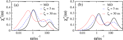
Figure 3: Loss spectra $\chi_{i}^{\prime\prime}(\omega)/\chi_{i}^{\prime}(0)$ of individual residues ($i=21$, a) and of pairs of residues $\chi_{ij}^{\prime\prime}(\omega)/\chi_{ij}^{\prime}(0)$ ($i=21$ and $j=84$, b). The results have been obtained from MD (solid lines) and DENM (dashed lines). The calculations are done for cytB with the residues used in the calculations shown in Fig. 4. The DENM calculations are done with $\zeta_{l}=30$ ns used for the electrostatic calculations in Fig. 5 (red dashed line) and with $\zeta_{l}=5$ ns (blue dash-dotted line). The rest of DENM parameters are: $\zeta_{h}=0.006\zeta_{l}$, $a=0.35$, $\varepsilon=100$.

The elastic network with single-exponential, Debye dynamics does not capture two time-scales of the dynamics from MD simulations. When the Debye memory kernel $\tilde{\zeta}(\omega)=\zeta_{0}$ is used in the response function $\chi_{m}(\omega)$ in Eqs. (4) and (5), the loss function shows only one relaxation peak, slightly deformed from a simple Debye form by the distribution of network’s eigenvalues $\lambda_{m}$. A single friction coefficient evidently misses the fact that energy dissipation decreases with increasing frequency of vibrations. Since the protein network is characterized by two spring constants, lower for non-covalent neighbors within the cutoff and higher for covalent neighbors, it must possess at least two characteristic friction coefficients.

Friction kernels typically used in applications are phenomenological (47) and we as well cannot offer a consistent theoretical formalism capturing the complex dynamics of residue displacements. We have therefore adopted a phenomenological response function best describing the MD results. Instead of searching for a functional form of $\tilde{\zeta}(\omega)$ reproducing MD simulations, we have resorted to a two-Debye form for the entire response function of bead displacements in Eq. (4)

$$\chi_{m}(\omega)=\frac{a}{i\omega\zeta_{h}+\lambda_{m}}+\frac{1-a}{i\omega\zeta_{l}+\lambda_{m}}.$$ (21)

Here, the amplitude $a$ represents the relative weight of the high-frequency dissipation with the high-frequency friction $\zeta_{h}$. Correspondingly, $\zeta_{l}$ is the low-frequency friction, which is larger in magnitude. It is obvious that Eq. (21) satisfies the static limit $\chi_{m}(0)=\lambda_{m}^{-1}$.

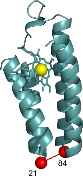
Figure 4: Cartoon of cytB showing the residues (red) used to produce the correlation functions $C_{i}(t)$ ($i=21$) and $C_{ij}(t)$ ($i,j=21,84$, Eqs. (19) and (20)) and corresponding loss spectra $\chi_{i}^{\prime\prime}(\omega)$ and $\chi_{ij}^{\prime\prime}(\omega)$ shown in Fig. 3. The residues used in producing $\chi_{ij}^{\prime\prime}(\omega)$ are connected by the red solid line. The red spheres representing the two chosen residues are centered at their corresponding $C^{\alpha}$ carbons. The Fe atom of the heme is rendered as a yellow sphere.

The two-Debye form of $\chi_{m}(\omega)$ is directly applied to calculate the response function of residue displacements

$$\chi_{ij}(\omega)=\chi_{ij}^{\alpha\alpha}(\omega),$$ (22)

where the function $\chi_{ij}^{\alpha\beta}(\omega)$ is given by Eq. (5). The loss spectra of residue displacements show two peaks and qualitatively agree with the simulations. The positions and relative heights of the peaks can be adjusted by choosing $\zeta_{h,l}$ and the amplitude $a$ in Eq. (21), as is illustrated in Fig. 3a by dashed and dash-dotted lines. The model can therefore be well parameterized to reproduce the dynamics of displacements of a small subset of residues. However, it fails to discriminate between the dynamics of residues across the protein backbone.

The loss functions calculated from MD for a number of residues (see Supporting Materials) display similar two-peaks pattern, but the weights and positions of their peaks vary among the residues. In contrast, the dynamics of displacements of individual residues in the elastic network are mostly driven by the global motions of the entire network. As a result, there is little difference between the loss functions of individual residues calculated with DENM. The same statement applies to the dynamics of distances between residues shown in Fig. 3b. While one can reproduce the loss function of a chosen pair of residues by adjusting the parameters of $\chi_{m}(\omega)$ in Eq. (21), these parameters do not translate to all pairs in the network and instead can be only viewed as an average representation of the pairs dynamics.

The fast component of the dynamics, prominent in the loss function $\chi_{X}^{\prime\prime}(\omega)$, is less significant in the function $\alpha_{X}(\omega)$ due to the $1/\omega$ scaling of $\chi_{X}^{\prime\prime}(\omega)$ in Eq. (16). The function $\alpha_{X}(\omega)$ is more relevant to problems related to the generalized compliance as defined by Eq. (14). The correct representation of the fast dynamics is therefore of lesser importance for these type of problems. The $1/\omega$ scaling difference between $\chi_{X}^{\prime\prime}(\omega)$ and $\alpha_{X}(\omega)$ explains the relative success of the network models in reproducing the pattern of residue msd’s (Fig. 2). Those are obtained by frequency integration of $\alpha_{r}(\omega)$ and are less sensitive to the details of local dynamics of individual beads in the network represented by high-frequency peak of their loss functions.

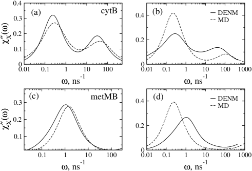
Figure 5: Loss spectra $\chi_{\phi}^{\prime\prime}(\omega)/\chi^{\prime}_{\phi}(0)$ (a,c) and $\chi_{E}^{\prime\prime}(\omega)/\chi_{E}^{\prime}(0)$ (b,d) for cytB (a,b) and metMB (c,d). The results are from MD trajectories (dashed lines) and from the DENM calculations (solid lines). The DENM calculations were done with the two-Debye $\chi_{m}(\omega)$ in Eq. (21). The two-Debye relaxation parameters are: $\zeta_{l}=30$ ns, $\zeta_{h}=0.006\zeta_{l}$, $a=0.35$ for cytB and $\zeta_{l}=10$ ns, $\zeta_{h}=0.0002\zeta_{l}$, $a=0.35$ for metMB. The elastic network is defined with $k_{\text{B}}T/C=1$ Ų, $\varepsilon=100$, and the cutoff radius of 15 Å.

Dynamics of the electrostatic field and potential

Essentially all time correlation functions obtained here from MD simulations show a pattern that is roughly represented by a two-exponential decay, requiring in some cases a third decaying exponent for a better mathematical fit. The relative weights of the fast and slow components of the correlation functions differ depending on the observable. The loss function of the electric field $\chi_{E}^{\prime\prime}(\omega)$ at the position of protein’s heme is mostly single-exponential, with the low-frequency peak much exceeding the high-frequency one. This pattern is less uniform for the loss function of the electrostatic potential showing different weights of the low- and high-frequency peaks in $\chi_{\phi}^{\prime\prime}(\omega)$ among the proteins (35). Figure 5 shows the loss spectra $\chi_{X}^{\prime\prime}(\omega)/\chi_{X}^{\prime}(0)$ calculated from the DENM and MD for cytB and metMB proteins. Similarly to the case with the residue displacements, the low-frequency coefficient needs adjustment to reproduce the position of the main loss peak: the value of $\zeta_{l}=30$ ns was adopted for cytB and $\zeta_{l}=10$ ns was taken for metMB. Still, the set of parameters taken to reproduce the loss spectrum of electrostatic potential does not perform as well when applied to the electric field (cf. Figs. 5c and 5d).

The relative contribution of the fast dynamics component is reduced in the spectral function $\alpha_{X}(\omega)$ describing the frequency variation of the generalized compliance (Eqs. (14 and (16)). Figure 6 compares $\alpha_{X}(\omega)$ from DENM with MD data for all three globular proteins studied here. In order to show the ability of DENM to describe the entire set of MD data, a single set of network and friction parameters has been assigned to all three proteins. As expected, the performance of DENM is better for $\alpha_{X}(\omega)$. The average relaxation time $\langle\tau\rangle$, given by the $\omega\rightarrow 0$ limit of $\alpha_{X}(\omega)$ (Eq. (17)), is well reproduced by the network calculations. The deviations for some observables correspond to the cases when the dynamics are strongly dominated by its high-frequency component. For these cases, the fit can be improved by adjusting the weight $a$ of the fast component in Eq. (21) to a higher value.

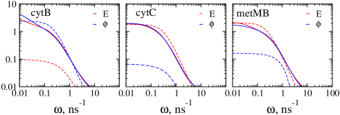
Figure 6: Functions $\alpha_{X}(\omega)$ (ns) for cytB, cytC, and metMB from MD (dashed lines) and DENM (solid lines). The results for the electrostatic potential ($\alpha_{\phi}(\omega)$, blue) and electric filed ($\alpha_{E}(\omega)$, red) are shown. A single set of network parameters is used for all three heme proteins: $\zeta_{l}=30$ ns, $\zeta_{h}=0.006\zeta_{l}$, $a=0.35$, $\varepsilon=100$.

The loss functions $\chi_{X}(\omega)$ shown in Figs. 3, 5, and 6 are normalized with the corresponding values of $\chi_{X}^{\prime}(0)$ and therefore are not affected by the magnitude of the spring constant $C$ describing the non-covalent interactions within the cutoff distance $r_{c}=15$ Å. The absolute values of the variances are, however, proportional to $k_{\text{B}}T/C$, as for instance in Eq. (2). We adopted in our calculations the value of $k_{\text{B}}T/C=1$ Ų, which is equivalent to $C\simeq 0.6$ kcal/(mol Ų). The results of calculating the generalized compliances $\lambda_{X}$ for electrostatic observables (Eqs. (14) and (15)) with this choice of the force constant are summarized in Table 1. The agreement is semi-quantitative at best. While the value of the force constant can clearly be adjusted in each particular case, this change does not propagate into equally good agreement between $\lambda_{\phi}$ and $\lambda_{F}$, where $F=eE$ is the electrostatic force acting on the unit charge placed at Fe of the heme. The requirement to reproduce electrostatic forces might be more stringent than to describe the electrostatic potential because of a shorter range and higher sensitivity to the local structure of the former. Since the statistical variances listed in Table 1 are not affected by the modeling of dissipative dynamics, the properties of the network itself need to be further fine-tuned. The inclusion of softening of the residue displacements by electrostatic water fluctuations (14) appears to be the first avenue for the model improvement. This addition will allow one to accommodate for the effect of the interface, in addition to the motions dictated by the shape and mass distribution which elastic models capture in the first place (28, 29, 30). Incorporating the water response will effectively produce a more heterogeneous distribution of the network force constants.

Table 1: Generalized compliances (Eq. (14)) for the electrostatic potential fluctuations $\lambda_{\phi}$ (also known as reorganization energies of redox half reaction $\lambda=e^{2}\lambda_{\phi}$, kcal/mol) and for the electric force, $F=eE$ ($\lambda_{F}$, kcal/(mol Ų)) for the three proteins used in the case study; the network is assigned the force constant of $C=0.6$ kcal/(mol Ų) for non-covalent springs and $\varepsilon C$, $\varepsilon=100$ for covalently bound neighbors. The cutoff radius is 15 Å.

Protein	$e^{2}\lambda_{\phi}$ (DENM)	$e^{2}\lambda_{\phi}$ (MD)	$\lambda_{F}$ (DENM)	$\lambda_{F}$ (MD)
MetMB	85	228	436	243
CytB	115	136	9	17
CytC	141	159	18	83

CONCLUSIONS

Network models of biomolecules are coarse-grained representations designed to describe their large-scale collective conformational motions (27). They capture the basic topology and packing of residues in a biopolymer and robustly reproduce conformational global motions driven by the distribution of mass and shape (28, 29, 30). Electrostatic properties is yet another area where coarse-graining of biomolecules might be efficient. The long range of Coulomb interactions effectively averages out details of the local structure suggesting that one can potentially describe the statistics and long-time dynamics of electrostatic fluctuations by global motions of charges assigned to the elastic network. The demonstration that this approach is in principle consistent with all-atom MD simulations is the main result of this study. Two components are critical to our approach: force-field atomic charges distributed at the residues of the network and two-exponential, overdamped dynamics assigned to each normal mode diagonalizing the network Hessian.

Harmonic mechanical motions of the network of beads clearly do not incorporate dissipative dynamics of biomolecules in solution (45, 46, 34) and much is still needed to be done to achieve a physically consistent description of the protein dynamics. The elastic network employed here assigns weaker springs between all non-covalent neighbors within a cutoff radius and stronger springs between covalent neighbors. Correspondingly, two global friction coefficients are assigned to each normal mode diagonalizing the network Hessian. This phenomenological model qualitatively captures the two-peak loss spectrum of residue displacements and qualitatively similar loss spectra of the electrostatic potential and electric field. However, the characteristic adjustable friction coefficients used for the electrostatic fluctuations are not transferrable to the network displacements. A new set of parameters is needed when each property is considered separately.

This research was supported by the National Science Foundation (DVM, CHE-0910905). CPU time was provided by the National Science Foundation through TeraGrid resources (TG-MCB080116N).

References

- Fenimore et al. (2004) Fenimore, P. W., H. Frauenfelder, B. H. McMahon, and R. D. Young, 2004. Bulk-solvent and hydration-shell fluctuations, similar to and -fluctuations in glasses, control protein motion and functions. Proc. Natl. Acad. Sci. 101:14408–14413.
- Henzlel-Wildman and Kern (2007) Henzlel-Wildman, K., and D. Kern, 2007. Dynamic personalities of proteins. Nature 450:964.
- Frauenfelder et al. (2009) Frauenfelder, H., G. Chen, J. Berendzen, P. W. Fenimore, H. Jansson, B. H. McMahon, I. R. Stroe, J. Swenson, and R. D. Young, 2009. A unified model of protein dynamics. Proc. Natl. Acad. Sci. 106:5129–5134.
- Marlow et al. (2010) Marlow, M. S., J. Dogan, K. K. Frederick, K. G. Valentine, and A. J. Wand, 2010. The role of conformational entropy in molecular recognition by calmodulin. Nat Chem Biol 6:352–358. http://dx.doi.org/10.1038/nchembio.347.
- Warshel et al. (2006) Warshel, A., P. K. Sharma, M. Kato, and W. W. Parson, 2006. Modeling electrostatic effects in proteins. Biochim. Biophys. Acta 1764:1647–1676.
- Marcus and Sutin (1985) Marcus, R. A., and N. Sutin, 1985. Electron transfer in chemistry and biology. Biochim. Biophys. Acta 811:265–322.
- LeBard and Matyushov (2010a) LeBard, D. N., and D. V. Matyushov, 2010. Protein-water electrostatics and principles of bioenergetics. Phys. Chem. Chem. Phys. 12:15335.
- Khodadadi et al. (2010) Khodadadi, S., J. H. Roh, A. Kisliuk, E. Mamontov, M. Tyagi, S. A. Woodson, R. M. Briber, and A. P. Sokolov, 2010. Dynamics of Biological Macromolecules: Not a Simple Slaving by Hydration Water. Biophys. J. 98:1321–1326.
- Ebbinghaus et al. (2007) Ebbinghaus, S., S. J. Kim, M. Heyden, X. Yu, U. Heugen, M. Gruebele, D. M. Leitner, and M. Havenith, 2007. An extended dynamical hydration shell around proteins. Proc. Natl. Acad. Sci. 104:20749–20752.
- Perticaroli et al. (2010) Perticaroli, S., L. Comez, M. Paolantoni, P. Sassi, L. Lupi, D. Fioretto, A. Paciaroni, and A. Morresi, 2010. Broadband depolarized light scattering study of diluted protein aqueous solutions. J. Phys. Chem. B 114:8262.
- Richardson and Richardson (2002) Richardson, J. S., and D. C. Richardson, 2002. Natural -sheet proteins use negative design to avoid edge-to-edge aggregation. Proc. Natl. Acad. Sci. 99:2754.
- Lawrence et al. (2007) Lawrence, M. S., K. J. Phillips, and D. R. Liu, 2007. Supercharging Proteins Can Impart Unusual Resilience. J. Am. Chem. Soc. 129:10110.
- Pace et al. (2009) Pace, C. N., G. R. Grimsley, and J. M. Scholtz, 2009. Protein ionizable groups: pK values and their contribution to protein stability and solubility. J. Biol. Chem. 284:13285.
- Matyushov and Morozov (2011) Matyushov, D. V., and A. Y. Morozov, 2011. Electrostatic fluctuations promote dynamical transition in proteins. Phys. Rev. E 84:011908.
- Andreatta et al. (2005) Andreatta, D., J. L. Pérez, S. A. Kovalenko, N. P. Ernsting, C. J. Murphy, R. S. Coleman, and M. A. Berg, 2005. Power-law solvation dynamics in DNA over six decades in time. J. Am. Chem. Soc. 127:7270.
- Tripathy and Beck (2010) Tripathy, J., and W. F. Beck, 2010. Nanosecond-Regime Correlation Time Scales for Equilibrium Protein Structural Fluctuations of Metal-Free Cytochrome c from Picosecond Time-Resolved Fluorescence Spectroscopy and the Dynamic Stokes Shift. J. Phys. Chem. B 114:15958–15968.
- Zhang et al. (2007) Zhang, L., L. Wang, Y.-T. Kao, W. Qiu, Y. Yang, O. Okobiah, and D. Zhong, 2007. Mapping hydration dynamics around a protein surface. Proc. Natl. Acad. Sci. 104:18461.
- Tirion (1996) Tirion, M. M., 1996. Large amplitude elastic motions from single-parameter, atomic analysis. Phys. Rev. Lett. 77:1905–1908.
- Atilgan et al. (2001) Atilgan, A. R., S. R. Durell, R. L. Jernigan, M. C. Demirel, O. Keskin, and I. Bahar, 2001. Anisotropy of Fluctuation Dynamics of Proteins with an Elastic Network Model. Biophys. J. 80:505–515.
- Tama and Sanejouand (2001) Tama, F., and Y. H. Sanejouand, 2001. Conformational change of proteins arising from normal mode calculations. Protein Eng 14:1–6.
- Tama et al. (2003) Tama, F., M. Valle, J. Frank, and r. Brooks, C. L., 2003. Dynamic reorganization of the functionally active ribosome explored by normal mode analysis and cryo-electron microscopy. Proc. Natl. Acad. Sci. USA 100:9319–23.
- Tama and Brooks (2005) Tama, F., and C. L. Brooks, 2005. Diversity and identity of mechanical properties of icosahedral viral capsids studied with elastic network normal mode analysis. J. Mol. Biol. 345:299–314.
- Lu et al. (2006) Lu, M., B. Poon, and J. Ma, 2006. A New Method for Coarse-Grained Elastic Normal-Mode Analysis. J. Chem. Theory Comput. 2:464–471.
- Moritsugu and Smith (2007) Moritsugu, K., and J. C. Smith, 2007. Coarse-Grained Biomolecular Simulation with REACH: Realistic Extension Algorithm via Covariance Hessian. Biophys. J. 93:3460–3469.
- Lu and Ma (2008) Lu, M., and J. Ma, 2008. A minimalist network model for coarse-grained normal mode analysis and its application to biomolecular x-ray crystallography. Proc. Nat. Acad. Sci. 105:15358–63.
- Riccardi et al. (2009) Riccardi, D., Q. Cui, and G. N. Phillips, 2009. Application of elastic network models to proteins in the crystalline state. Biophys. J. 96:464–475.
- Bahar et al. (2010) Bahar, I., T. R. Lezon, L.-W. Yang, and E. Eyal, 2010. Global Dynamics of Proteins: Bridging Between Structure and Function. Ann. Rev. Biophys. 39:23–42.
- Halle (2002) Halle, B., 2002. Flexibility and packing in proteins. Proc. Natl. Acad. Sci. 99:1274–1279.
- Lu and Ma (2005) Lu, M., and J. Ma, 2005. The Role of Shape in Determining Molecular Motions. Biophys. J. 89:2395–2401.
- Tama and Brooks (2006) Tama, F., and C. L. Brooks, 2006. Symmetry, Form, and Shape: Guiding Principles for Robustness in Macromolecular Machines. Annu. Rev. Biophys. Biomol. Struct. 35:115–133.
- Petrone and Pande (2006) Petrone, P., and V. S. Pande, 2006. Can conformational change be described by only a few normal modes? Biophys. J. 90:1583–1593.
- Lyman et al. (2008) Lyman, E., J. Pfaendtner, and G. A. Voth, 2008. Systematic multiscale parametrization of heterogeneous elastic network models of proteins. Biophys. J. 95:4183.
- Hinsen and Kneller (1999) Hinsen, K., and G. R. Kneller, 1999. A simplified force field for describing vibrational protein dynamics over the whole frequency range. J. Chem. Phys. 111:10766–10769.
- Miller et al. (2008) Miller, B. T., W. Zheng, R. M. Venable, R. W. Pastor, and B. R. Brooks, 2008. Langevin Network Model of Myosin. J. Phys. Chem. B 112:6274–6281.
- Matyushov (2011) Matyushov, D. V., 2011. Nanosecond Stokes Shift Dynamics, Dynamical Transition, and Gigantic Reorganization Energy of Hydrated Heme Proteins. J. Phys. Chem. B 115:10715–10724.
- LeBard and Matyushov (2009) LeBard, D. N., and D. V. Matyushov, 2009. Energetics of bacterial photosynthesis. J. Phys. Chem. B 113:12424–12437.
- Tozzini (2010) Tozzini, V., 2010. Minimalist models for proteins: a comparative analysis. Quarterly Reviews of Biophysics 43:333–371.
- Hinsen (2008) Hinsen, K., 2008. Structural flexibility in proteins: impact of the crystal environment. Bioinformatics 24:521–8.
- Gerek and Ozkan (2011) Gerek, Z. N., and S. B. Ozkan, 2011. Change in allosteric network affects binding affinities of PDZ Domains: Analysis through Perturbation Response Scanning. PLoS Comput. Biol. 7:e1002154.
- Ming and Wall (2005) Ming, D., and M. E. Wall, 2005. Allostery in a Coarse-Grained Model of Protein Dynamics. Phys. Rev. Lett. 95:198103.
- Gerek et al. (2009) Gerek, Z. N., O. Keskin, and S. B. Ozkan, 2009. Identification of specificity and promiscuity of PDZ domain interactions through their dynamic behavior. Proteins 77:796–811.
- Smith (1991) Smith, J. C., 1991. Protein dynamics: comparison of simulations with inelastic neutron scattering experiments. Quat. Rev. Biophys. 24:227.
- Cametti et al. (2011) Cametti, C., S. Marchetti, C. M. C. Gambi, and G. Onori, 2011. Dielectric Relaxation Spectroscopy of Lysozyme Aqueous Solutions: Analysis of the delta-Dispersion and the Contribution of the Hydration Water. J. Phys. Chem. B 115:7144–7153.
- Lamm and Szabo (1986) Lamm, G., and A. Szabo, 1986. Langevine modes of macromolecules. J. Chem. Phys. 85:7334.
- Ansari (1999) Ansari, A., 1999. Langevin modes analysis of myoglobin. J. Chem. Phys. 110:1774–1780.
- Erkip and Erman (2004) Erkip, A., and B. Erman, 2004. Dynamics of large-scale fluctuations in native proteins. Analysis based on harmonic inter-residue potentials and random external noise. Polymer 45:641–648.
- Hansen and McDonald (2003) Hansen, J. P., and I. R. McDonald, 2003. Theory of Simple Liquids. Academic Press, Amsterdam.
- Essiz and Coalson (2009) Essiz, S. G., and R. D. Coalson, 2009. Dynamic Linear Response Theory for Conformational Relaxation of Proteins. J. Phys. Chem. B 113:10859–10869.
- Soheilifard et al. (2011) Soheilifard, R., D. E. Makarov, and G. J. Rodin, 2011. Rigorous coarse-graining for the dynamics of linear systems with applications to relaxation dynamics in proteins. J. Chem. Phys. 135.
- Skepö et al. (2006) Skepö, M., P. Linse, and T. Arnebrant, 2006. Coarse-Grained Modeling of Proline Rich Protein 1 (PRP-1) in Bulk Solution and Adsorbed to a Negatively Charged Surface. J. Phys. Chem. B 110:12141–12148.
- Pizzitutti et al. (2007) Pizzitutti, F., M. Marchi, and D. Borgis, 2007. Coarse-Graining the Accessible Surface and the Electrostatics of Proteins for Protein-Protein Interactions. J. Chem. Theory and Comp. 3:1867–1876.
- Leherte and Vercauteren (2009) Leherte, L., and D. P. Vercauteren, 2009. Coarse Point Charge Models For Proteins From Smoothed Molecular Electrostatic Potentials. J. Chem. Theory Comp. 5:3279–3298.
- Dong et al. (2008) Dong, F., B. Olsen, and N. A. Baker, 2008. Methods in Cell Biology, Elsevier, volume 84, chapter Computational methods for biomolecular electrostatics, 843.
- Berardi et al. (2004) Berardi, R., L. Muccioli, S. Orlandi, M. Ricci, and C. Zannoni, 2004. Mimicking electrostatic interactions with a set of effective charges: a genetic algorithm. Chemical Physics Letters 389:373–378.
- Chaikin and Lubensky (1995) Chaikin, P. M., and T. C. Lubensky, 1995. Principles of condensed matter physics. Cambridge University Press, Cambridge.
- LeBard and Matyushov (2008) LeBard, D. N., and D. V. Matyushov, 2008. Redox Entropy of Plastocyanin: Developing a Microscopic View of Mesoscopic Solvation. J. Chem. Phys. 128:155106.
- MacKerell et al. (1998) MacKerell, A. D., D. Bashford, M. Bellott, R. L. D. Jr., J. D. Evanseck, M. J. Field, S. Fischer, J. Gao, H. Guo, D. S. Ha, J. McCarthy, L. Kuchnir, K. Kuczera, F. T. K. Lau, C. Mattos, S. Michnick, T. Ngo, D. T. Nguyen, B. Prodhom, W. E. R. III, B. Roux, M. Schlenkrich, J. C. Smith, R. Stote, J. Straub, M. Watanabe, J. Wirkiewicz-Kuczera, D. Yin, and M. Karplus, 1998. All-atom empirical potential for molecular modeling and dynamics studies of proteins. J. Phys. Chem. B 102:3586–3616.
- Phillips et al. (2005) Phillips, J. C., R. Braun, W. Wang, J. Gumbart, E. Tajkhorshid, E. Villa, C. Chipot, R. D. Skeel, L. Kale, and K. Schulten, 2005. Scalable molecular dynamics with NAMD. J. Comp. Chem. 26:1781–1802.
- Jorgensen et al. (1983) Jorgensen, W. L., J. Chandrasekhar, J. D. Madura, R. W. Impey, and M. L. Klein, 1983. Comparison of simple potential functions for simulating liquid water. J. Chem. Phys. 79:926–935.
- Humphrey et al. (1996) Humphrey, W., A. Dalke, and K. Schulten, 1996. VMD - Visual Molecular Dynamics. Journal of Molecular Graphics 14:33–38.
- LeBard and Matyushov (2010b) LeBard, D. N., and D. V. Matyushov, 2010. Ferroelectric hydration shells around proteins: Electrostatics of the protein-water interface. J. Phys. Chem. B 114:9246–9258.
- Autenrieth et al. (2004) Autenrieth, F., E. Tajkhorshid, J. Baudry, and Z. Luthney-Schulten, 2004. Classical force field parameters for the heme prosthetic group of cytochrome c. J. Comp. Chem. 25:1613.
- Meuwly et al. (2002) Meuwly, M., O. M. Becker, R. Stote, and M. Karplus, 2002. NO rebinding to myoglobin: a reactive molecular dynamics study. Biophys. Chem. 98:183.
- Zhang and Straub (2009) Zhang, Y., and J. E. Straub, 2009. Diversity of solvent dependent energy transfer pathways in heme proteins. J. Phys. Chem. B 113:825.
- Gabel et al. (2002) Gabel, F., D. Bicout, U. Lehnert, M. Tehei, M. Weik, and G. Zaccai, 2002. Protein dynamics studied by neutron scattering. Quat. Rev. Biophys. 35:327–367.
- Zaccai (2000) Zaccai, G., 2000. How soft is a protein? A protein dynamics force constant measured by neutron scattering. Science 288:1604–1607.
- Weiss (2000) Weiss, S., 2000. Measuring conformational dynamics of biomolecules by single molecule fluorescence spectroscopy. Nat. Struct. Biol. 7:724 – 729.