Photon Structure Function in Supersymmetric QCD Revisited

Abstract

We investigate the virtual photon structure function in the supersymmetric QCD (SQCD), where we have squarks and gluinos in addition to the quarks and gluons. Taking into account the heavy particle mass effects to the leading order in QCD and SQCD we evaluate the photon structure function and numerically study its behavior for the QCD and SQCD cases.

Since the experiments at the Large Hadron Collider (LHC) [1] started there has been much anticipation for the signals of the Higgs boson as well as for an evidence of the new physics beyond Standard Model such as supersymmetry (SUSY). Once these signals are observed more precise measurement needs to be carried out at the future $e^{+}e^{-}$ collider, so called International Linear Collider (ILC) [2]. In such a case, it is important to know the theoretical predictions at high energies based on QCD.

It is well known that, in $e^{+}e^{-}$ collision experiments, the cross section for the two-photon processes $e^{+}e^{-}\rightarrow e^{+}e^{-}+{\rm hadrons}$ dominates at high energies over the one-photon annihilation process [3]. We consider here the two-photon processes in the double-tag events where both of the outgoing $e^{+}$ and $e^{-}$ are detected. Especially, the case in which one of the virtual photon is far off-shell (large $Q^{2}\equiv-q^{2}$), while the other is close to the mass-shell (small $P^{2}=-p^{2}$), with $\Lambda^{2}\ll P^{2}\ll Q^{2}$ ($\Lambda$: QCD scale parameter), can be viewed as a deep-inelastic scattering where the target is a virtual photon and we can calculate the photon structure functions in perturbation theories  [4, 5, 6, 7, 8, 9, 10, 11, 12].

Figure 1: $e^{+}~{}e^{-}$ two-photon processes in supersymmetric QCD. The solid (dashed) line denotes the quark (squark), while the spiral (spiral-straight) line implies the gluon (gluino).

Some time ago the effects of supersymmetry on two-photon process were studied in the literature [13, 14, 15, 16]. In this paper based on the framework of treating heavy parton distributions [17, 18] we reexamine the effects of the squarks and gluinos appearing in SUSY QCD (SQCD) on the photon structure functions to the leading order in SQCD which can be measured in the two-photon processes of $e^{+}e^{-}$ collision illustrated in Fig.1.

1 Evolution equations for the SUSY QCD

We consider the DGLAP type evolution equations for the parton distribution functions inside the virtual photon with the mass squared, $P^{2}$, in SQCD where we have squarks and gluinos in addition to the ordinary quarks and gluons. Evolution equation to the leading order (LO) in SQCD reads as in QCD [19]:

$$\frac{d\mbox{\boldmath$q$}^{\gamma}(t)}{dt}=\mbox{\boldmath$q$}^{\gamma}(t)\otimes P^{(0)}+\frac{\alpha}{\alpha_{s}(t)}\mbox{\boldmath$k$}^{(0)}~{},$$ (1)

where $P^{(0)}$ and $\mbox{\boldmath$k$}^{(0)}$ are 1-loop parton-parton and photon-parton splitting functions, respectively (see Appendix). The symbol $\otimes$ denotes the convolution between the splitting function and the parton distribution function. The variable $t$ is defined in terms of the running coupling $\alpha_{s}$ as [20]:

$$t=\frac{2}{\beta_{0}}\ln\frac{\alpha_{s}(P^{2})}{\alpha_{s}(Q^{2})},\quad\frac{d\alpha_{s}(Q^{2})}{d\ln{Q^{2}}}=-\beta_{0}\frac{\alpha_{s}(Q^{2})^{2}}{4\pi}+{\cal O}(\alpha_{s}(Q^{2})^{3})$$ (2)

with the parton distributions probed by the virtual photon with mass squared $Q^{2}$ as

$$\mbox{\boldmath$q$}^{\gamma}(t)=(G,\lambda,q_{1},\cdots q_{n_{f}},s_{1},\cdots,s_{n_{f}}),$$ (3)

where $n_{f}$ is the number of active flavors. In eq.(2), $\beta_{0}=9-n_{f}$ for SQCD. We denote the distribution function of the $i$-th flavor quark, squark by $q_{i}(x,Q^{2},P^{2})$, $s_{i}(x,Q^{2},P^{2})$, ($i=1,\cdots,n_{f}$), and the gluon, gluino by $G(x,Q^{2},P^{2})$, $\lambda(x,Q^{2},P^{2})$, respectively. The 1-loop splitting functions were obtained in [21, 22]. We first consider the case where all the particles are massless. Although this is an unrealistic case, it is instructive to consider the massless case for the later treatment of the realistic case with the heavy mass effects.

For the massless partons the evolution starts at $Q^{2}=P^{2}$ and hence we have the initial condition $\mbox{\boldmath$q$}^{\gamma}(t=0)=0~{}$[11].

The 1-loop splitting function is given by (see Appendix A)

$$P^{(0)}=\left(\begin{array}[]{cccc}P_{GG}&P_{\lambda G}&P_{qG}&P_{sG}\\ P_{G\lambda}&P_{\lambda\lambda}&P_{q\lambda}&P_{s\lambda}\\ P_{Gq}&P_{\lambda q}&P_{qq}&P_{sq}\\ P_{Gs}&P_{\lambda s}&P_{qs}&P_{ss}\end{array}\right)~{},$$ (8)

where $P_{AB}$ is a splitting function of $B$ parton to $A$ parton with $A,B=G,\lambda,q$ and $s$. While the splitting functions of the photon into the partons $G,\lambda,q$ and $s$, are denoted as (see Appendix B)

$$\mbox{\boldmath$k$}^{(0)}=(k_{G},k_{\lambda},k_{q},k_{s})~{}.$$ (9)

We introduce the flavor-nonsinglet (NS) combinations of the quark and squark distribution functions as

$$q_{NS}(x,Q^{2},P^{2})=\sum_{i=1}^{n_{f}}(e_{i}^{2}-\langle e^{2}\rangle)q_{i}(x,Q^{2},P^{2})~{},$$ (10)

$$s_{NS}(x,Q^{2},P^{2})=\sum_{i=1}^{n_{f}}(e_{i}^{2}-\langle e^{2}\rangle)s_{i}(x,Q^{2},P^{2})~{},$$ (11)

where $e_{i}$ is the $i$-th flavor charge and $\langle e^{2}\rangle=\sum_{i}e_{i}^{2}/n_{f}$ is the average charge squared. We also define the flavor-singlet (S) combinations for quarks and squarks

$$\Sigma(x,Q^{2},P^{2})=\sum_{i=1}^{n_{f}}q_{i}(x,Q^{2},P^{2})~{},$$ (12)

$$S(x,Q^{2},P^{2})=\sum_{i=1}^{n_{f}}s_{i}(x,Q^{2},P^{2})~{}.$$ (13)

We now rearrange the parton components of $\mbox{\boldmath$q$}^{\gamma}(t)$ using the above flavor non-singlet and singlet combinations as:

$$\mbox{\boldmath$q$}^{\gamma}(t)=(G,\lambda,\Sigma,S,q_{NS},s_{NS})~{}.$$ (14)

Then we have the following splitting function

$$P^{(0)}=\left(\begin{array}[]{cccc|cc}P_{GG}&P_{\lambda G}&P_{qG}&P_{sG}&&\\ P_{G\lambda}&P_{\lambda\lambda}&P_{q\lambda}&P_{s\lambda}&&\smash{\hbox{\bg 0}}\\ P_{Gq}&P_{\lambda q}&P_{qq}&P_{sq}&&\\ P_{Gs}&P_{\lambda s}&P_{qs}&P_{ss}&&\\ \hline\cr&&&&P_{qq}&P_{sq}\\ &\smash{\hbox{\bg 0}}&&&P_{qs}&P_{ss}\end{array}\right)~{}.$$ (21)

Thus for the flavor-nonsinglet parton distributions

$$\mbox{\boldmath$q$}_{NS}^{\gamma}=(q_{NS},s_{NS})~{},$$ (22)

satisfy the following evolution equation:

$$\frac{d\mbox{\boldmath$q$}_{NS}^{\gamma}}{dt}=\mbox{\boldmath$q$}_{NS}^{\gamma}\otimes P^{(0)}_{NS}+\frac{\alpha}{\alpha_{s}(t)}\mbox{\boldmath$k$}^{(NS)}~{},$$ (23)

where the splitting functions are

$$P^{(0)}_{NS}=\left(\begin{array}[]{cc}P_{qq}&P_{sq}\\ P_{qs}&P_{ss}\end{array}\right),\ \mbox{\boldmath$k$}^{(NS)}=(K_{q}^{(NS)},K_{s}^{(NS)}),$$ (26)

$$K_{q}^{(NS)}=\sum_{i=1}^{n_{f}}(e_{i}^{2}-\langle e^{2}\rangle)k_{q_{i}},\ K_{s}^{(NS)}=\sum_{i=1}^{n_{f}}(e_{i}^{2}-\langle e^{2}\rangle)k_{s_{i}}~{}.$$ (27)

For the flavor-singlet parton distribution

$$\mbox{\boldmath$q$}_{S}^{\gamma}=(G,\lambda,\Sigma,S)~{},$$ (28)

we have

$$\frac{d\mbox{\boldmath$q$}_{S}^{\gamma}}{dt}=\mbox{\boldmath$q$}_{S}^{\gamma}\otimes P^{(0)}_{S}+\frac{\alpha}{\alpha_{s}(t)}\mbox{\boldmath$k$}^{(S)}~{},$$ (29)

where

$$P^{(0)}_{S}=\left(\begin{array}[]{cccc}P_{GG}&P_{\lambda G}&P_{qG}&P_{sG}\\ P_{G\lambda}&P_{\lambda\lambda}&P_{q\lambda}&P_{s\lambda}\\ P_{Gq}&P_{\lambda q}&P_{qq}&P_{sq}\\ P_{Gs}&P_{\lambda s}&P_{qs}&P_{ss}\end{array}\right)~{},$$ (34)

$$\mbox{\boldmath$k$}^{(S)}=(K_{q}^{(S)},K_{s}^{(S)}),\ K_{q}^{(S)}=\sum_{i=1}^{n_{f}}k_{q_{i}},\ K_{s}^{(S)}=\sum_{i=1}^{n_{f}}k_{s_{i}}.$$ (35)

Now we should notice that there exist the following supersymmetric relations for the splitting functions [21]:

$$P_{qq}+P_{sq}=P_{qs}+P_{ss}\equiv P_{\phi\phi},$$ (36)

$$P_{qG}+P_{sG}=P_{q\lambda}+P_{s\lambda}\equiv P_{\phi V},$$ (37)

$$P_{Gq}+P_{\lambda q}=P_{Gs}+P_{\lambda s}\equiv P_{V\phi},$$ (38)

$$P_{GG}+P_{\lambda G}=P_{G\lambda}+P_{\lambda\lambda}\equiv P_{VV}~{}.$$ (39)

Hence if we introduce the following combinations

$$\hskip 28.45274pt\phi\equiv\Sigma+S,\quad V\equiv G+\lambda,$$ (40)

then we obtain the following compact form for the mixing of the flavor-singlet part:

$$\frac{d\phi}{dt}=P_{\phi\phi}\otimes\phi+P_{\phi V}\otimes V+\frac{\alpha}{\alpha_{s}(t)}K_{\phi}^{(S)},$$ (41)

$$\frac{dV}{dt}=P_{V\phi}\otimes\phi+P_{VV}\otimes V,$$ (42)

where we denote $K_{\phi}^{(S)}=K_{q}^{(S)}+K_{s}^{(S)}$ and the flavor-nonsinglet part $\phi_{NS}=q_{NS}+s_{NS}$ becomes

$$\frac{d\phi_{NS}}{dt}=P_{\phi\phi}\otimes\phi_{NS}+\frac{\alpha}{\alpha_{s}(t)}K_{\phi}^{(NS)},$$ (43)

where we introduced $K_{\phi}^{(NS)}=K_{q}^{(NS)}+K_{s}^{(NS)}$. In terms of the flavor singlet and non-singlet parton distribution functions we can express the virtual photon structure function $F_{2}^{\gamma}$ as

$$F_{2}^{\gamma}(x,Q^{2},P^{2})=x\sum_{i}e_{i}^{2}(q_{i}(x,Q^{2},P^{2})+s_{i}(x,Q^{2},P^{2}))$$ (44)

$$= x\sum_{i}(e_{i}^{2}-\langle e^{2}\rangle)(q_{i}(x,Q^{2},P^{2})+s_{i}(x,Q^{2},P^{2}))$$

$$+x\langle e^{2}\rangle\sum_{i}(q_{i}(x,Q^{2},P^{2})+s_{i}(x,Q^{2},P^{2}))$$

$$= x(q_{NS}(x,Q^{2},P^{2})+s_{NS}(x,Q^{2},P^{2}))$$

$$+x\langle e^{2}\rangle(\Sigma(x,Q^{2},P^{2})+S(x,Q^{2},P^{2}))$$

$$= x\phi_{NS}(x,Q^{2},P^{2})+x\langle e^{2}\rangle\phi(x,Q^{2},P^{2})$$

In Fig.2 we have plotted the virtual photon structure function $F_{2}^{\gamma}(x,Q^{2},P^{2})$ in the SQCD as well as in the ordinary QCD for $Q^{2}=(1000)^{2}$GeV² and $P^{2}=(10)^{2}$GeV². We have also shown the quark as well as the squark components of the virtual photon structure function $F_{2}^{\gamma}$ in the case of the SQCD. In contrast to the QCD, the momentum fraction carried by the quarks in the SQCD case decreases due to the emission of the squarks and the gluinos. Hence the $x$-distribution of the quarks for the SQCD increases at small-$x$ and decreases at large $x$, i.e. it becomes more flat compared to the QCD case as seen from the Fig.2. Adding the two components together we get the $F_{2}^{\gamma}$ structure function for the SQCD which shows a behavior quite different from that of the QCD.

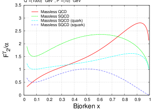
Figure 2: The virtual photon structure function $F_{2}^{\gamma}(x,Q^{2},P^{2})$ divided by the QED coupling constant $\alpha$ for massless QCD (solid line) and SQCD (dashed line) with $n_{f}=6$, $Q^{2}=(1000)^{2}$GeV² and $P^{2}=(10)^{2}$GeV². Also shown are the quark (dash-dotted line) and the squark (double-dotted line) components.

2 Heavy parton mass effects

Many authors have studied heavy quark mass effects in the nucleon [23] and the photon structure functions [24, 25, 26]. Now we consider the heavy parton mass effects, and we decompose the parton distributions in the case where we have $n_{f}-1$ light quarks and one heavy quark flavor which we take the $n_{f}$-th quark and all the squarks have the same heavy mass, while the gluino has another heavy mass [17, 18]:

$$\mbox{\boldmath$q$}^{\gamma}(t)=(G,\lambda,q_{1},\cdots,q_{n_{f}-1},s_{1},\cdots,s_{n_{f}-1},q_{H},s_{H})~{}.$$ (45)

We denote the $i$-th light flavor quark, squark by $q_{i}(x,Q^{2},P^{2})$, $s_{i}(x,Q^{2},P^{2})$, ($i=1,\cdots,n_{f}-1$), one heavy quark and its superpartner (squark) by $q_{H}$, $s_{H}$ and the gluon, gluino by $G(x,Q^{2},P^{2})$, $\lambda(x,Q^{2},P^{2})$, respectively.

We now define light flavor-nonsinglet (LNS) and singlet (LS) combination of the quark and the squark as follows:

$$q_{LNS}=\sum_{i=1}^{n_{f}-1}\left(e_{i}^{2}-\langle e^{2}\rangle_{L}\right)q_{i},\quad s_{LNS}=\sum_{i=1}^{n_{f}-1}\left(e_{i}^{2}-\langle e^{2}\rangle_{L}\right)s_{i}~{},$$

$$q_{LS}=\sum_{i=1}^{n_{f}-1}q_{i},\quad s_{LS}=\sum_{i=1}^{n_{f}-1}s_{i},\quad\langle e^{2}\rangle_{L}=\frac{1}{n_{f}-1}\sum_{i=1}^{n_{f}-1}e_{i}^{2}~{}.$$ (46)

Then we rearrange the parton distributions as

$$\mbox{\boldmath$q$}^{\gamma}(t)=(G,\lambda,q_{LS},s_{LS},q_{H},s_{H},q_{LNS},s_{LNS})~{}.$$ (47)

The evolution equations and the splitting functions read

$$\frac{d\mbox{\boldmath$q$}^{\gamma}(t)}{dt}=\mbox{\boldmath$q$}^{\gamma}(t)\otimes P^{(0)}+\frac{\alpha}{\alpha_{s}(t)}\mbox{\boldmath$k$}^{(0)}~{},\quad P^{(0)}=\left(\begin{array}[]{c|c}P^{LS}&0\\ \hline\cr 0&P^{LNS}\end{array}\right)~{},$$ (50)

$$P^{LS}\equiv\left(\begin{array}[]{cccccc}P_{GG}&P_{\lambda G}&\frac{n_{f}-1}{n_{f}}P_{qG}&\frac{n_{f}-1}{n_{f}}P_{sG}&\frac{1}{n_{f}}P_{qG}&\frac{1}{n_{f}}P_{sG}\\ P_{G\lambda}&P_{\lambda\lambda}&\frac{n_{f}-1}{n_{f}}P_{q\lambda}&\frac{n_{f}-1}{n_{f}}P_{s\lambda}&\frac{1}{n_{f}}P_{q\lambda}&\frac{1}{n_{f}}P_{s\lambda}\\ P_{Gq}&P_{\lambda q}&P_{qq}&P_{sq}&0&0\\ P_{Gs}&P_{\lambda s}&P_{qs}&P_{ss}&0&0\\ P_{Gq}&P_{\lambda q}&0&0&P_{qq}&P_{sq}\\ P_{Gs}&P_{\lambda s}&0&0&P_{qs}&P_{ss}\end{array}\right),$$ (57)

$$P^{LNS}\equiv\left(\begin{array}[]{cc}P_{qq}&P_{sq}\\ P_{qs}&P_{ss}\end{array}\right)~{}.$$ (60)

While the photon-parton splitting functions are

$$\mbox{\boldmath$k$}^{(0)}=(k_{G},k_{\lambda},k_{q_{LS}},k_{s_{LS}},k_{q_{H}},k_{s_{H}},k_{q_{LNS}},k_{s_{LNS}})~{}.$$ (61)

Now we take into account the heavy mass effects by setting the initial conditions for the heavy parton distribution functions as discussed in [18, 27, 28].

We note here that the structure function $F_{2}^{\gamma}$ can be written as a convolution of the parton distribution $\mbox{\boldmath$q$}^{\gamma}(x,Q^{2},P^{2})$ and the Wilson coefficient function $\mbox{\boldmath$C$}(x,Q^{2})$:

$$F_{2}^{\gamma}(x,Q^{2},P^{2})/x=\mbox{\boldmath$q$}^{\gamma}\otimes\mbox{\boldmath$C$}~{}.$$ (62)

The moments of the parton distributions are defined as

$$\mbox{\boldmath$q$}^{\gamma}(n,t)\equiv\int_{0}^{1}dxx^{n-1}\mbox{\boldmath$q$}^{\gamma}(x,Q^{2},P^{2})~{},$$ (63)

where we put the initial conditions:

$$\mbox{\boldmath$q$}^{\gamma}(n,t=0)=\left(0,\hat{\lambda}(n),0,\hat{s}_{LS}(n),\hat{q}_{H}(n),\hat{s}_{H}(n),0,\hat{s}_{LNS}(n)\right)~{},$$ (64)

and require that the following boundary conditions are satisfied:

$$\lambda(n,Q^{2}=m_{\lambda}^{2})=0,\ s_{LS}(n,Q^{2}=m_{sq}^{2})=0,\ q_{H}(n,Q^{2}=m_{H}^{2})=0,$$

$$s_{H}(n,Q^{2}=m_{sq}^{2})=0,\ s_{LNS}(n,Q^{2}=m_{sq}^{2})=0,$$ (65)

where $m_{\lambda}$, $m_{sq}$ and $m_{H}$ are the mass of the gluino, squarks and the heavy (here we take top) quark, respectively. Note that here we take all the squarks have the same mass $m_{sq}$.

By solving the evolution equation taking into account the above boundary condition we get for the moment of $\mbox{\boldmath$q$}^{\gamma}$:

$$\mbox{\boldmath$q$}^{\gamma}(n,t)=\frac{\alpha}{8\pi\beta_{0}}\frac{4\pi}{\alpha_{s}(t)}\mbox{\boldmath$K$}_{n}^{(0)}\sum_{i}P^{n}_{i}\frac{1}{1+d^{n}_{i}}\left\{1-\left[\frac{\alpha_{s}(t)}{\alpha_{s}(0)}\right]^{1+d^{n}_{i}}\right\}$$

$$\hskip 71.13188pt+\mbox{\boldmath$q$}^{\gamma}(n,0)\sum_{i}P^{n}_{i}\left[\frac{\alpha_{s}(t)}{\alpha_{s}(0)}\right]^{d^{n}_{i}}~{},$$ (66)

where the $P^{n}_{i}$ is the projection operator onto the eigenstate $\lambda_{i}$ of the anomalous dimension matrices $\hat{\gamma}_{n}$:

$$\hat{\gamma}_{n}=\sum_{i}P^{n}_{i}\lambda^{n}_{i}~{},$$ (67)

where the anomalous dimension matrices $\hat{\gamma}_{n}$ is related to the splitting function $P(x)$ as

$$\hat{\gamma}_{n}\equiv-2\int_{0}^{1}dxx^{n-1}P(x),\quad$$ (68)

and $d^{n}_{i}\equiv\lambda^{n}_{i}/2\beta_{0}$. $\mbox{\boldmath$K$}^{(0)}_{n}$ is the anomalous dimension corresponding to the photon-parton splitting function:

$$\mbox{\boldmath$K$}^{(0)}_{n}=2\int_{0}^{1}dxx^{n-1}\mbox{\boldmath$k$}^{0}(x)~{}.$$ (69)

The initial value $\mbox{\boldmath$q$}^{\gamma}(n,0)$ is determined so that we have

$$q_{j}^{\gamma}(t=t_{m_{j}})=0,\quad t_{m_{j}}=\frac{2}{\beta_{0}}\ln\frac{\alpha_{s}(P^{2})}{\alpha_{s}(m_{j}^{2})}~{},$$ (70)

or

$$0=\frac{4\pi}{\alpha_{s}(t_{m_{j}})}\sum_{i}\left(\mbox{\boldmath$K$}_{n}^{(0)}P^{n}_{i}\right)_{j}\frac{1}{1+d^{n}_{i}}\left\{1-\left[\frac{\alpha_{s}(m_{j}^{2})}{\alpha_{s}(P^{2})}\right]^{1+d^{n}_{i}}\right\}$$

$$\hskip 28.45274pt+\sum_{i}\left(\mbox{\boldmath$q$}^{\gamma}(n,0)/\frac{\alpha}{8\pi\beta_{0}}P^{n}_{i}\right)_{j}\left[\frac{\alpha_{s}(m_{j}^{2})}{\alpha_{s}(P^{2})}\right]^{d^{n}_{i}}~{},$$ (71)

for $j=\lambda,s_{LS},q_{H},s_{H}$ and $s_{LNS}$. By solving the above coupled equations we get the initial condition: $\mbox{\boldmath$q$}^{\gamma}(n,0)=(0,\hat{\lambda}(n),0,\hat{s}_{LS}(n),\hat{q}_{H}(n),\hat{s}_{H}(n),0,\hat{s}_{LNS}(n))$.

Now we write down the moments of the structure function in terms of the parton distribution functions and the coefficient functions, which are ${\cal O}(\alpha_{s}^{0})$ at LO. We take

$$\mbox{\boldmath$C$}^{(0)}_{n}(1,0)^{T}=(0,0,\langle e^{2}\rangle_{L},\langle e^{2}\rangle_{L},e_{H}^{2},e_{H}^{2},1,1)~{}.$$ (72)

Then the $n$-th moment of the structure function $F_{2}^{\gamma}$ to the leading order in SQCD is given by

$$M_{n}^{\gamma}=\int_{0}^{1}dxx^{n-1}F_{2}^{\gamma}/x=\mbox{\boldmath$q$}^{\gamma}(n)\cdot\mbox{\boldmath$C$}^{\gamma}_{n}(1,0)$$

$$=\langle e^{2}\rangle_{L}q_{LS}+\langle e^{2}\rangle_{L}s_{LS}+e_{H}^{2}q_{H}^{2}+e_{H}^{2}s_{H}+q_{LNS}+s_{LNS}~{}.$$ (73)

3 Numerical analysis

We have solved the equations (71) for $\mbox{\boldmath$q$}^{\gamma}(n,0)$ numerically, and plug them into the master formula (66) for the parton distribution functions and then evaluate the moments of the structure function $F_{2}^{\gamma}$ based on the formula (73). By inverting the Mellin moment we get the $F_{2}^{\gamma}$ as a function of Bjorken $x$.

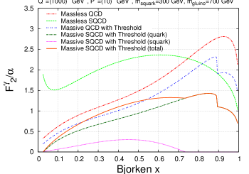
Figure 3: $F_{2}^{\gamma}(x,Q^{2},P^{2})/{\alpha}$ with SUSY particles as well as top threshold included. The dashed (2dot-dashed) curve corresponds to the massless SQCD (QCD) case. The double-dotted curve shows the massive QCD case. The dash-dotted (dotted) curve corresponds to the quark (squark) component of the massive QCD. The solid curve means the $F_{2}^{\gamma}/\alpha$ for the massive SQCD. The kink at $x$=0.89 (0.74) corresponds to the top (squark) threshold.

In Fig. 3, we have plotted our numerical results for the $F_{2}^{\gamma}/\alpha$. The 2dot-dashed and dashed curves correspond to the $F_{2}^{\gamma}/\alpha$ for the massless QCD and SQCD, respectively, where all the quarks and squarks are taken to be massless. Of course this is the unrealistic case we discussed in the previous section. For the more realistic case, we take $n_{f}=6$ and treat the $u$, $d$, $s$, $c$ and $b$ to be massless and take the top quark $t$ massive. We assume that all the squarks possess the same heavy mass and the gluino has another heavy mass. In these analyses, we have taken $Q^{2}=(1000)^{2}$GeV² and $P^{2}=(10)^{2}$GeV². For the mass values we took the top mass $m_{\rm top}=175$ GeV, the common squark mass, $m_{s}=300$ GeV and the gluino mass $m_{\lambda}=700$ GeV.

The double-dotted curve shows $F_{2}^{\gamma}/\alpha$ for the QCD with the mass of the top quark as well as the threshold effects taken into account. The dash-dotted curve shows the quark component for the massive SQCD case with massive top quark, while the dotted curve means the squark component for the same case. The sum of these leads to the solid curve which corresponds to $F_{2}^{\gamma}/\alpha$ for the massive SQCD with massive top and threshold effects included. Here, we adopt the prescription for taking into account the threshold effects by rescaling the argument of the distribution function $f(x)$ as [29]:

$$f(x)\rightarrow f(x/x_{\rm max})~{},\quad x_{\rm max}=\frac{1}{1+\frac{P^{2}}{Q^{2}}+\frac{4m^{2}}{Q^{2}}}$$ (74)

where $x_{\rm max}$ is the maximal value for the Bjorken variable. After this substitution the range of $x$ becomes $0\leq x\leq x_{\rm max}$. At small $x$, there is no significant difference between massless and massive QCD, while there exists a large difference between massless and massive SQCD. At large $x$, the significant mass-effects exist both for non-SUSY and SUSY QCD. The SQCD case is seen to be much suppressed at large $x$ compared to the QCD. The squark contribution to the total structure function in massive SQCD appears as a broad bump for $x<x_{\rm max}$. Here of course we could set the squark mass larger than 300 GeV, e.g. around 1 TeV, as recently reported by the ATLAS/CMS group at LHC, for higher values of $Q^{2}$.

4 Conclusion

In this paper we have studied the virtual photon structure function in the framework of the parton evolution equations for the supersymmetric QCD, where we have PDFs for the squarks and gluinos in addition to those for the quarks and gluons.

We considered the heavy parton mass effects for the top quark, squarks and gluinos by imposing the boundary conditions for their PDFs in the framework treating heavy particle distribution functions [18]. The PDF for the heavy particle with mass squared, $m^{2}$ are required to vanish at $Q^{2}=m^{2}$. This can be translated into the initial condition for the heavy parton PDFs, $\mbox{\boldmath$q$}^{\gamma}(t=0)$. Due to the initial condition the solution to the evolution equation is altered as given by (66). This change leads to the heavy mass effects for the PDFs. As we have shown in Fig.3, there is no significant difference in the small-$x$ region between QCD and SQCD, while at large $x$, it turns out that there exists a sizable difference between the massive QCD and SQCD. When compared to the squark contribution to $F_{2}^{\gamma}$ in the parton model calculation [30], the squark component in the SQCD is suppressed at large $x$ due to the radiative correction. We expect that the future linear collider would enable such an analysis to be carried out on photon structure functions.

Appendix A Anomalous Dimensions for SUSY QCD

Note that the our convention for the anomalous dimension is related to the above splitting function as

$$\gamma_{ij}^{n}=-2\int_{0}^{1}dxx^{n-1}P_{ij}(x)~{}.$$ (75)

The 1-loop anomalous dimensions for SUSY QCD are given by

$$\gamma_{qq}^{n}=2C_{F}\left[-2-\frac{2}{n(n+1)}+4S_{1}(n)\right],$$

$$\gamma_{sq}^{n}=2C_{F}\left[\frac{-2}{n+1}\right],$$

$$\gamma_{qs}^{n}=2C_{F}\left[\frac{-2}{n}\right],$$

$$\gamma_{ss}^{n}=2C_{F}\left[-2+4S_{1}(n)\right],$$

$$\gamma_{qG}^{n}=-4n_{f}\frac{n^{2}+n+2}{n(n+1)(n+2)},$$

$$\gamma_{sG}^{n}=-4n_{f}\frac{2}{(n+1)(n+2)}=-8n_{f}\frac{1}{(n+1)(n+2)},$$

$$\gamma_{q\lambda}^{n}=-4n_{f}\left[\frac{1}{n}-\frac{1}{n+1}\right],$$

$$\gamma_{s\lambda}^{n}=-4n_{f}\left(\frac{1}{n+1}\right),$$

$$\gamma_{Gq}^{n}=-4C_{F}\frac{n^{2}+n+2}{n(n^{2}-1)},$$

$$\gamma_{\lambda q}^{n}=-4C_{F}\frac{1}{n(n+1)},$$

$$\gamma_{Gs}^{n}=-4C_{F}\left[\frac{2}{n-1}-\frac{2}{n}\right],$$

$$\gamma_{\lambda s}^{n}=-4C_{F}\frac{1}{n},$$

$$\gamma_{GG}^{n}=2C_{A}\left[-3-\frac{4}{n(n-1)}-\frac{4}{(n+1)(n+2)}+4S_{1}(n)\right]+2n_{f},$$

$$\gamma_{\lambda G}=-4C_{A}\frac{n^{2}+n+2}{n(n+1)(n+2)}=-12\frac{n^{2}+n+2}{n(n+1)(n+2)},$$

$$\gamma_{G\lambda}^{n}=-4C_{A}\left[\frac{2}{n-1}-\frac{2}{n}+\frac{1}{n+1}\right],$$

$$\gamma_{\lambda\lambda}=2C_{A}\left[-3-\frac{2}{n}+\frac{2}{n+1}+4S_{1}(n)\right],$$ (76)

where $C_{F}=4/3$ and $C_{A}=3$ for SQCD. Hence we have the following anomalous dimensions for the supersymmetric case:

$$\gamma_{\phi\phi}^{n}=\gamma_{qq}^{n}+\gamma_{sq}^{n}=\gamma_{qs}^{n}+\gamma_{ss}^{n}=2C_{F}\left[-2-\frac{2}{n}+4S_{1}(n)\right],$$

$$\gamma_{\phi V}^{n}=\gamma_{qG}^{n}+\gamma_{sG}^{n}=\gamma_{q\lambda}^{n}+\gamma_{s\lambda}^{n}=-4n_{f}\frac{1}{n},$$

$$\gamma_{V\phi}^{n}=\gamma_{Gq}^{n}+\gamma_{\lambda q}^{n}=\gamma_{Gs}^{n}+\gamma_{\lambda s}^{n}=-4C_{F}\left[\frac{2}{n-1}-\frac{1}{n}\right],$$

$$\gamma_{VV}^{n}=\gamma_{GG}^{n}+\gamma_{\lambda G}^{n}=\gamma_{G\lambda}^{n}+\gamma_{\lambda\lambda}^{n}$$

$$=2C_{A}\left[-3-\frac{4}{n-1}+\frac{2}{n}+4S_{1}(n)\right]+2n_{f},$$ (77)

where we have the following replacement: $n_{f}\gamma_{\phi V}^{n}\rightarrow\gamma_{\phi V}^{n}$. In the case of non-supersymmetric QCD we have the following anomalous dimensions:

$$\gamma_{\psi\psi}^{0,n}=\gamma_{NS}^{0,n}=\frac{8}{3}\left[-3-\frac{2}{n(n+1)}+4S_{1}(n)\right],$$

$$\gamma_{\psi G}^{0,n}=-4n_{f}\frac{n^{2}+n+2}{n(n+1)(n+2)},$$

$$\gamma_{G\psi}^{0,n}=-\frac{16}{3}\frac{n^{2}+n+2}{n(n^{2}-1)},$$

$$\gamma_{GG}^{0,n}=6\left[-\frac{11}{3}-\frac{4}{n(n-1)}-\frac{4}{(n+1)(n+2)}+4S_{1}(n)\right]$$

$$\hskip 142.26378pt+\frac{4}{3}n_{f}.$$ (78)

Appendix B Photon-parton mixing anomalous dimensions

The photon-parton splitting function can be connected to the photon-parton mixing anomalous dimensions given by

$$\mbox{\boldmath$K$}^{(0)}_{n}=\left(K^{0,n}_{G},K^{0,n}_{\lambda},K^{0,n}_{q_{LS}},K^{0,n}_{s_{LS}},K^{0,n}_{q_{H}},K^{0,n}_{s_{H}},K^{0,n}_{q_{LNS}},K^{0,n}_{s_{LNS}}\right),$$

where

$$K^{0,n}_{G}=K^{0,n}_{\lambda}=0,$$

$$K^{0,n}_{q_{LS}}=24(n_{f}-1)\langle e^{2}\rangle_{L}\frac{n^{2}+n+2}{n(n+1)(n+2)},$$

$$K^{0,n}_{s_{LS}}=24(n_{f}-1)\langle e^{2}\rangle_{L}\left[\frac{1}{n}-\frac{n^{2}+n+2}{n(n+1)(n+2)}\right],$$

$$K^{0,n}_{q_{H}}=24e_{H}^{2}\frac{n^{2}+n+2}{n(n+1)(n+2)},$$

$$K^{0,n}_{s_{H}}=24e_{H}^{2}\left[\frac{1}{n}-\frac{n^{2}+n+2}{n(n+1)(n+2)}\right],$$

$$K^{0,n}_{q_{LNS}}=24(n_{f}-1)\left(\langle e^{4}\rangle_{L}-\langle e^{2}\rangle_{L}^{2}\right)\frac{n^{2}+n+2}{n(n+1)(n+2)},$$

$$K^{0,n}_{s_{LNS}}=24(n_{f}-1)\left(\langle e^{4}\rangle_{L}-\langle e^{2}\rangle_{L}^{2}\right)\left[\frac{1}{n}-\frac{n^{2}+n+2}{n(n+1)(n+2)}\right].$$

References

[1]
http://lhc.web.cern.ch/lhc.
[2]
http://www.linearcollider.org/cms.
[3]
T. F. Walsh,
Phys. Lett. 36 B (1971) 121;
S. J. Brodsky, T. Kinoshita and H. Terazawa,
Phys. Rev. Lett. 27 (1971) 280.
[4]
M. Krawczyk, A. Zembrzuski and M. Staszel,
Phys. Rept. 345 (2001) 265;
R. Nisius,
Phys. Rept. 332 (2000) 165;
M. Klasen,
Rev. Mod. Phys. 74 (2002) 1221;
I. Schienbein,
Ann. Phys. 301 (2002) 128;
R. M. Godbole,
Nucl. Phys. Proc. Suppl. 126 (2004) 414.
[5]
T. F. Walsh and P. M. Zerwas,
Phys. Lett. 44 B (1973) 195;
R. L. Kingsley,
Nucl. Phys. B 60 (1973) 45.
[6]
E. Witten,
Nucl. Phys. B 120 (1977) 189.
[7]
W. A. Bardeen and A. J. Buras,
Phys. Rev. D 20 (1979) 166;
21 (1980) 2041(E).
[8]
G. Altarelli,
Phys. Rep. 81 (1982) 1.
[9]
R. J. DeWitt, L. M. Jones, J. D. Sullivan, D. E. Willen
and H. W. Wyld, Jr., Phys. Rev. D 19 (1979) 2046;
D 20 (1979) 1751(E).
[10]
M. Glück and E. Reya,
Phys. Rev. D 28 (1983) 2749.
[11]
T. Uematsu and T. F. Walsh,
Phys. Lett. 101 B (1981) 263;
Nucl. Phys. B 199 (1982) 93.
[12]
G. Rossi,
Phys. Rev. D 29 (1984) 852;
F. M. Borzumati and G. A. Schuler,
Z. Phys. C 58 (1993) 139;
M. Drees and R. M. Godbole, Phys. Rev. D50
(1994) 3124;
P. Mathews and V. Ravindran, Int. J. Mod. Phys. A11,
(1996) 2783;
J. Chýla, Phys. Lett. B488 (2000) 289.
[13]
E. Reya,
Phys. Lett. B124 (1983) 424.
[14]
D. A. Ross and L. J. Weston,
Eur. Phys. JC18 (2001) 593.
[15]
M. Drees, M. Glück and E. Reya,
Phys. Rev. D30 (1984) 2316.
[16]
I. Antoniadis, C. Kounnas and R. Lacaze,
Nucl. Phys. B211 (1983) 216.
[17]
Y. Kitadono, K. Sasaki, T. Ueda and T. Uematsu,
Prog. Theor. Phys. 121 (2009) 495;
Phys. Rev. D81 (2010) 074029;
Y. Kitadono, Phys. Lett. B702 (2011) 135.
[18]
Y. Kitadono, R. Sahara, T. Ueda and T. Uematsu,
Eur. Phys. J. C70 (2010) 999.
[19]
K. Sasaki and T. Uematsu,
Phys. Rev.D59 (1999) 114011.
[20]
W. Furmanski and R. Petronzio,
Z. Phys.C11 (1982) 293.
[21]
C. Kounnas and D. A. Ross,
Nucl. Phys. B214 (1983) 317.
[22]
S. K. Jones and C. H. Llewellyn Smith,
Nucl. Phys.B217 (1983) 145.
[23]
M. Buza, Y. Matiounine, J. Smith, R. Migneron and W. L. van Neerven,
Nucl. Phys. B 472 (1996) 611;
I. Birenbaum, J. Blümlein and S. Klein,
Nucl. Phys. B 780 (2007) 40;
820 (2009) 417.
[24]
M. Glück, E. Reya and M. Stratmann,
Phys. Rev. D 51 (1995) 3220;
D 54 (1996) 5515;
M. Glück, E. Reya and I. Schienbein,
Phys. Rev. D 60 (1999) 054019;
D 62 (2000) 019902(E);
Phys. Rev. D 63 (2001) 074008.
[25]
K. Sasaki, J. Soffer and T. Uematsu,
Phys. Rev. D 66 (2002) 034014.
[26]
F. Cornet, P. Jankowski, M. Krawczyk and A. Lorca,
Phys. Rev. D 68 (2003) 014010;
F. Cornet, P. Jankowski and M. Krawczyk,
Phys. Rev. D 70 (2004) 093004.
[27]
M. Fontannaz, Eur. Phys. J. C38 (2004) 297;
[28]
P. Aurenche, M. Fontannaz and J. P. Guillet,
Z. Phys. C64(1994) 621;
Eur. Phys. J. C44 (2005) 395;
[29]
M. Aivazis, J. C. Collins, F. Olness and W. K. Tung,
Phys. Rev. D50 (1994) 3102.
[30]
Y. Kitadono, Y. Yoshida, R. Sahara and T. Uematsu,
Phys. Rev. D84 (2011) 074031.