IRIE: Scalable and Robust Influence Maximization
in Social Networks

Abstract

Influence maximization is the problem of selecting top $k$ seed nodes in a social network to maximize their influence coverage under certain influence diffusion models. In this paper, we propose a novel algorithm IRIE that integrates a new message passing based influence ranking (IR), and influence estimation (IE) methods for influence maximization in both the independent cascade (IC) model and its extension IC-N that incorporates negative opinion propagations. Through extensive experiments, we demonstrate that IRIE matches the influence coverage of other algorithms while scales much better than all other algorithms. Moreover IRIE is more robust and stable than other algorithms both in running time and memory usage for various density of networks and cascade size. It runs up to two orders of magnitude faster than other state-of-the-art algorithms such as PMIA for large networks with tens of millions of nodes and edges, while using only a fraction of memory comparing with PMIA.

1 Introduction

Word-of-mouth or viral marketing has long been acknowledged as an effective marketing strategy. The increasing popularity of online social networks such as Facebook and Twitter provides opportunities for conducting large-scale online viral marketing in these social networks. Two key technology components that would enable such large-scale online viral marketing is modeling influence diffusion and influence maximization. In this paper, we focus on the second component, which is the problem of finding a small set of $k$ seed nodes in a social network to maximize their influence spread — the expected total number of activated nodes after the seed nodes are activated, under certain influence diffusion models.

In particular, we study influence maximization under the classic independent cascade (IC) model [10] and its extension IC-N model incorporating negative opinions [2]. IC model is one of the most common information diffusion model which is widely used in economics, epidemiology, sociology, and so on [10]. Most of existing researches for the influence maximization problem are based on the IC model, assuming dynamics of information diffusion among individuals are independent. Kempe et al. originally proposed the IC model and a greedy approximation algorithm to solve the influence maximization problem under the IC model [10]. The greedy algorithm proceeds in rounds, and in each round one node with the largest marginal contribution to influence spread is added to the seed set. However, computing influence spread given a seed set is shown to be #P-hard [3], and thus the greedy algorithm has to use Monte-Carlo simulations with a large number of simulation runs to obtain an accurate estimate of influence spread, making it very slow and not scalable. A number of follow-up works tackle the problem by designing more efficient and scalable optimizations and heuristics [11, 13, 8, 4, 3, 8, 9]. Among them PMIA [3] algorithm has stood out as the most efficient heuristic so far, which runs three orders of magnitude faster than the optimized greedy algorithm of [13, 4], while maintaining good influence spread in par with the greedy algorithm.

In this paper, we propose a novel scalable influence maximization algorithm IRIE, and demonstrate through extensive simulations that IRIE scales even better than PMIA, with up to two orders of magnitude speedup and significant savings in memory usage, while maintaining the same level or even better influence spread than PMIA. We also demonstrate that while the running time of PMIA is very sensitive to structural properties of the network such as the clustering coefficient and the edge density, and to the cascade size, IRIE is much more stable and robust over them and always shows very fast running time. In the greedy algorithm as well as in PMIA, each round a new seed with the largest marginal influence spread is selected. To select this seed, the greedy algorithm uses Monte-Carlo simulations while PMIA uses more efficient local tree based heuristics to estimate marginal influence spread of every possible candidate. This is especially slow for the first round where the influence spread of every node needs to be estimated. Therefore, instead of estimating influence spread for each node at each round, we propose a novel global influence ranking method IR derived from a belief propagation approach, which uses a small number of iterations to generate a global influence ranking of the nodes and then select the highest ranked node as the seed. However, the influence ranking is only good for selecting one seed. If we use the ranking to directly select $k$ top ranked nodes as $k$ seeds, their influence spread may overlap with one another and not result in the best overall influence spread. To overcome this shortcoming, we integrate IR with a simple influence estimation (IE) method, such that after one seed is selected, we estimate additional influence impact of this seed to each node in the network, which is much faster than estimating marginal influence for many seed candidates, and then use the results to adjust next round computation of influence ranking. When combining IR and IE together, we obtain our fast IRIE algorithm. Besides being fast, IRIE has another important advantage, which is its memory efficiency. For example, PMIA needs to store data structures related to the local influence region of every node, and thus incurs a high memory overhead. In constrast, IRIE mainly uses global iterative computations without storing extra data structures, and thus the memory overhead is small.

We conduct extensive experiments using synthetic networks as well as five real-world networks with size ranging from $29K$ to $69M$ edges, and different IC model parameter settings. We compare IRIE with other state-of-the-art algorithms including the optimized greedy algorithm, PMIA, simulated annealing (SA) algorithm proposed in [9], and some baseline algorithms including the PageRank. Our results show that (a) for influence spread, IRIE matches the greedy algorithm and PMIA while being significantly better than SA and PageRank in a number of tests; and (b) for scalability, IRIE is some orders of magnitude faster than the greedy algorithm and PMIA and is comparable or faster than SA; and (c) for stability IRIE is much more stable and robust over structural properties of the network and the cascade size than PMIA and the greedy algorithm.

Moreover, to show the wide applicability of our IRIE approach, we also adapt IRIE to the IC-N model, which considers negative opinions emerging and propagating in networks [2]. Our simulation results again show that IRIE has comparable influence coverage while scales much better than the MIA-N heuristic proposed in [2].

Related Work. Domingo and Richardson [6] are the first to study influence maximization problem in probabilistic settings. Kempe et al. [10] formulate the problem of finding a subset of influential nodes as a combinatorial optimization problem and show that influence maximization problem is NP-hard. They propose a greedy algorithm which guarantees $(1-1/e)$ approximation ratio. However, their algorithm is very slow in practice and not scalable with the network size. In [13], [8], authors propose lazy-foward optimization that significantly speeds up the greedy algorithm, but it still cannot scale to large networks with hundreds of thousands of nodes and edges. A number of heuristic algorithms are also proposed [11, 4, 3, 15, 9] for the independent cascade model. SPM/SP1M of [11] is based on shortest-path computation, and SPIN of [15] is based on Shapley value computation. Both SPM/SP1M and SPIN have been shown to be not scalable [3, 5]. Simulated annealing approach is proposed in [9], which provides reasonable influence coverage and running time. The best heuristic algorithm so far is believed to be the PMIA algorithm proposed by Chen et al. [3], which provides matching influence spread while running at three orders of magnitude faster than the optimized greedy algorithm. PageRank [1] is a popular ranking algorithm for ranking web pages and other networked entities, and it considers diffusion processes whose corresponding transition matrix must have column sums equal to one. Hence it can not be directly used for the influence spread estimation. Our algorithm IR overcomes this shortcoming, and uses equations more directly designed for the IC model. More importantly, our IRIE algorithm integrates influence ranking with influence estimation together with the greedy approach, overcoming the general issue of ignoring overlapping influence coverages suffered by all pure ranking methods. Our simulation results also demonstrate that IRIE performs much better than PageRank in influence coverage. The IC-N model is proposed in [2] to consider the emergence and propagation of negative opinions due to product or service quality issues. A corresponding MIA-N algorithm, an extension of PMIA is proposed for influence maximization under IC-N. We show that our IRIE algorithm adapted to IC-N also outperforms MIA-N in scalability. Recently, Goyal et al. propose a data-based approach to social influence maximization [7]. They define a new propagation probability model called credit distribution model, which reveals how influence flows in the networks based on datasets and propose a novel algorithm for influence maximization for that model. Scalable algorithms for a related model called linear threshold model has also been studied [5]. It is a future work to see if our IRIE approach could be applied to further speed up scalable algorithms for the linear threshold model.

The rest of the paper is organized as follows. Section 2 describes problem statement and preliminaries. Section 3 provides our IRIE algorithm and its extension for IC-N model. Section 4 shows experimental results, and Section 5 contains the conclusion.

2 Model and Problem Setup

2.1 Influence Maximization Problem and IC Model

Influence Maximization problem [10] is a discrete optimization problem in a social network that chooses an optimal initial seed set of given size to maximize influence under a certain information diffusion model. In this paper, we consider Independent Cascade (IC) model as the information diffusion process. We first introduce IC model, then provide a formal definition of Influence Maximization problem under the IC model. Let $G=(V,E)$ be a directed graph for a social network and $P_{uv}\in[0,1]$ be an edge propagation probability assigned to each edge $(u,v)\in E$. Each node represents a user and each edge corresponds to a social relationship between a pair of users. In the IC model, each node has either an active or inactive state and is allowed to change its state from inactive to active, but not the reverse direction.

Given a seed set $S$, the process of IC model is as follows : At step $t=0$, all seed nodes $u\in S$ are activated and added to $S_{0}$. At each step $t>0$, a node $u\in S_{t-1}$ tries to affect its inactive out-neighbors $v\in N^{out}(u)$ with probability $P_{uv}$ and all the nodes activated at this step are added to $S_{t}$. This process ends at a step $t$ if $|S_{t}|=0$. Note that every activated node $u$ belongs to just one of $S_{i}$, where $i=0,1,...,t$. Hence, it has a single chance to activate its neighbors $v\in N^{out}(u)$ at the next step that it is activated. This activation of nodes models the spread of information among people by the word-of-mouth effect as a result of marketing campaigns. Under the IC model, let us define our influence function $\sigma(S)$ as the expected number of activated nodes given a seed set.

Formally, Influence Maximization problem is defined as follows : Given a directed social network $G=(V,E)$ and $P_{uv}$ for each edge $(u,v)\in E$, influence maximization problem is to select a seed set $S\subseteq V$ with $|S|=k$ that maximizes influence $\sigma(S)$ under the IC model. In [10], it is shown that the exact computation of optimum solution for this problem is NP-hard, but the Greedy algorithm achieves $(1-1/e)$ -approximation by proving the facts that the influence function $\sigma$ is non-negative, monotone, and submodular. A set function $f$ is called monotone if $f(S)\leq f(T)$ for all $S\subseteq T$, and the definition of submodular function is described at Definition 1.

Definition 1.

A set function $f:2^{V}\rightarrow R$ is submodular if for every $S\subseteq T\subseteq V$ and $v\in V$, $f(S\cup u)-f(S)\geq f(T\cup u)-f(T)$.

Theorem 1.

[10] For a non-negative, monotone, and submodular influence function $\sigma$, let S be a size-$k$ set obtained by the greedy hill-climbing algorithm in Algorithm 1. Then $S$ satisfies $\sigma(S)\geq(1-1/e)\cdot\sigma(S^{*})$ where $S^{*}$ is an optimum solution.

At each step, Algorithm 1 computes marginal influence of every node $u\in V\setminus S$ and then add the maximum one into the seed set $S$ until $|S|=K$. Although the greedy algorithm guarantees constant-approximation solutions and is easy to implement, computing the influence function $\sigma(S)$ is proven to be #P-hard [3]. To estimate influence function $\sigma(S)$, Monte-Carlo simulation has been used in many previous works [10, 13, 4, 8]. Although Monte-Carlo simulation provides the best accuracy among existing measures of influence function, the Greedy algorithm with Monte-Carlo simulation takes days or weeks in large networks with millions of nodes and edges. Many heuristic measures have been used to estimate influence function such as Shortest-path computation [11], Shapley value computation [15], Effective diffusion values [9], Degree discount [4], Community based computation [17]. They show much faster running time than the Monte-Carlo simulation, but result in lower accuracy than the Greedy algorithm. Hence, it is essential to design an algorithm that has the best trade-off between running time and accuracy. In this paper, we design a scalable, and memory efficient heuristic algorithm balancing running time and accuracy.

Algorithm 1 Greedy(K)

1:  initialize $S=\emptyset$

2:  for $i\leftarrow 1$ to $K$ do

3:     select $u\leftarrow argmax_{w\in V\setminus S}(\sigma(S\cup\{w\})-\sigma(S))$

4:     $S=S\cup\{u\}$

5:  end for

6:  output S

2.2 IC-N Model

We also provide a generalized version of our algorithm for Independent Cascade model with Negative Opinions (IC-N), which has been recently introduced in [2] to model the emergence and propagation of negative opinions caused by social interactions.

In the IC-N model, each node has one of three states, neutral, positive, and negative. Initially, every node $u\in V\setminus S$ has neutral state and may change its state during the diffusion process. We say that a node $v$ is activated at time $t$ if its state is neutral at time $(t-1)$ and becomes either positive or negative at time $t$. IC-N model has a parameter $q$ called quality factor which is a probability that a node is positively activated by a positive in-neighbor.

Given a seed set $S$, the IC-N model works as follows : Initially at time $t=0$, for each node $u\in S$, $u$ is activated positively with probability $q$ or negatively with probability $1-q$, independently of all other activations. At a step $t>0$, for any neutral node $v$, let $A_{t}(v)\subseteq N^{in}(v)$ be the set of in-neighbors of $v$ that are activated at step $t-1$ and $\pi_{t}(v)=$ $\langle u_{1},u_{2},...,u_{m}\rangle$ be a randomly permuted sequence of nodes $u_{i}$ where $u_{i}\in A_{t}(v),i=1,2,...,m$. Each node $u_{i}\in\pi_{t}(v)$ tries to activate $v$ with an independent probability $P_{u_{i}v}$ in the order of $\pi_{t}(v)$. This process ends at time $t$ when there is no activated node at time $(t-1)$.

If any node in $A_{t-1}(v)$ succeeds in activating $v$, $v$ is activated at step $t$ and becomes either positive or negative. The state of $v$ is decided by the following rules : If $v$ is activated by a negative node $u$, then $v$ becomes negative. If $v$ is activated by a positive node, it becomes positive with probability $q$, or negative with probability $1-q$. Those rules reflect negativity bias phenomenon — negative opinions usually dominate over positive opinions well known in social psychology [16].

In the IC-N model, the influence function of a seed set $S$ in a social network $G$ with quality factor $q$ is defined as the expected number of positive nodes activated in the graph, and is denoted as $\sigma_{G}(S,q)$. In [2], Chen et al. show that $\sigma_{G}(S,q)$ is always monotone, non-negative and submodular. Therefore, Algorithm 1 also guaranteeing $(1-1/e)$-approximation of an optimum solution for influence maximization problem under the IC-N model.

3 Our Algorithm

In this section, we describe our algorithms for influence maximization. As in the greedy algorithm and PMIA, at each round of IRIE, it selects a node $u$ with the largest marginal influence estimate $\sigma(S\cup\{u\})-\sigma(S)$. For a given seed set $S$, let $\sigma(u|S)=\sigma(S\cup\{u\})-\sigma(S)$. The Greedy algorithm estimates $\sigma(u|S)$ by a Monte-Carlo simulation and PMIA generates local tree structures for all $u\in V$ inducing slow running time. The novelty of our algorithm lies in that we derive a system of linear equations for $\{\sigma(u|S)\}_{u\in V}$ whose solution can be computed fast by an iterative method. Then we use these computed values as our estimates of $\{\sigma(u|S)\}_{u\in V}$.

3.1 Simple Influence Rank

We first explain our formula for $\{\sigma(u|S)\}_{u\in V}$ when $S=\emptyset$. Let $\sigma(u)=\sigma(u|\emptyset)$. The basic idea of our formula lies in that the influence of a node $u$ is essentially determined by the influences of $u$’s neighbors under the IC model. First suppose that graph $G=(V,E)$ is a tree graph. For $(v,u)\in E$, we define $m(u,v)$ to be the expected number of activated nodes when $S=\{u\}$ and $(u,v)$ is removed from $E$. Note that for a tree graph $G$, $m(u,v)$ is the expected influence from $u$ excluding the direction toward $v$. Let $\tilde{\sigma}(u)$ and $\tilde{m}(u,v)$ be our estimates of $\sigma(u)$ and $m(u,v)$ respectively. We compute $\tilde{\sigma}(u)$ and $\tilde{m}(u,v)$ from the following formulas.

$$\tilde{\sigma}(u)=1+\sum_{v\in N^{out}(u)}P_{uv}\cdot\tilde{m}(v,u),$$ (1)

$$\tilde{m}(u,v)=1+\left(\sum_{w\in N^{out}(u),w\neq v}P_{uw}\cdot\tilde{m}(w,u)\right).$$ (2)

Note that equation (2) forms a system of $|E|$ linear equations on $|E|$ variables. When $G$ is a tree, (2) has a unique solution. We prove correctness of (1) and (2) by Theorem 2. The proof of Theorem 2 is described in Appendix A.

Theorem 2.

For any tree graph, for each node $u$, $\tilde{\sigma}(u)=\sigma(u)$, and for each edge $(v,u)\in E$, $\tilde{m}(u,v)=m(v,u)$.

Even when $G$ is not a tree, we can define the same equations (1) and (2). In this case, the $\tilde{\sigma}(u)$ computed from 1) and (2) corresponds to the influence of $u$ when we allow multiple counts of influence from $u$ to each node via different paths. Note that this approach has a similarity with the popular Belief Propagation(BP) algorithm. As in the BP, one natural way to compute the solution of (1) and (2) is using an iterative message passing algorithm.

This iterative algorithm, which we call Influence Propagation (IP), is described in Algorithm 2.

Algorithm 2 Influence Propagation

1:  for all $(u,v)\in E$ do

2:     $\tilde{m}_{0}(u,v)\leftarrow 1$

3:  end for

4:  repeat

5:     $t\leftarrow t+1$

6:     for all $(v,u)\in E$ do

7:        $m_{t}(u,v)\leftarrow 1+\alpha\cdot(\sum_{w\in N^{out}(u),w\neq v}P_{uw}\cdot\tilde{m}_{t-1}(w,u))$

8:     end for

9:  until $\forall(u,v)\in E$, $\tilde{m}_{t}(u,v)=\tilde{m}_{t-1}(u,v)$

10:  for all $u\in V$ do

11:     $\tilde{\sigma}(u)\leftarrow 1+\sum_{v\in N^{out}(u)}P_{uv}\cdot\tilde{m}_{t}(v,u)$

12:  end for

Although IP computes good estimates of $\sigma(u)$ for tree and general graphs, its running time may be slow since one iteration of IP takes $O(\sum_{v\in V}d_{in}(v)\cdot d_{out}(v))$ time where $d_{in}(v)$ and $d_{out}(v)$ is the in-degree and out-degree of $v$ respectively. We observe that for most nodes $u$, $m(u,v)$’s are similar for any $v\in N^{in}(u)$ since the out-degree of $u$ is not too small. Based on this observation, by substituting the same variable $r(u)$ for all the $m(u,v)$, $v\in N^{in}(u)$, we obtain our formulas for the simplified expected influence $r(u)$ as follows :

$$r(u)=1+\left(\sum_{v\in N^{out}(u)}P_{uv}\cdot r(v)\right).$$ (3)

Note that equation (3) forms a system of $|V|$ linear equations on $|V|$ variables. Let $X=\left(r(u)\right)_{u\in V}$, and the influence matrix $A\in\mathbb{R}^{|V|\times|V|}$ be $A_{uv}=P_{uv}$. Let $B=(1,1,\ldots,1)^{T}\in\mathbb{R}^{|V|}$. Then (3) becomes

$$X=AX+B.$$ (4)

If $\lim\limits_{k\to\infty}A^{k}=0$, the solution of (4) becomes

$$\begin{split}&(I-A)X=B.\\ &(I+A+A^{2}+\cdots)(I-A)X=(I+A+A^{2}+\cdots)B.\end{split}$$

$$\therefore X=B+AB+A^{2}B+\cdots$$ (5)

Note that $(A^{k})_{uv}$ is the summation of the expectation of influence paths so that the diffusion process begins from a single node set $\{u\}$ and it activates a node $v$ after exactly $k$ number of iterations when we allow loops in the paths. Hence $(A^{k}\cdot B)_{u}$ is equal to the expectation of relaxed influence of node $u$ after exactly $k$ number of iterations where relaxed means that we allow multiple counts of influence on some nodes and loops in the paths.

Hence, from (5), $X_{u}$ is the expectation of relaxed influence of node $i$. Note that $X_{u}$ is an upper bound of $\sigma(u)$ for all $u\in V$. Here we assumed that $\lim\limits_{k\to\infty}A^{k}=0$. Note that otherwise there can appear a large spreading (constant fraction of nodes becomes influenced) even if the diffusion process begins from a single node. It is known that in most real world information diffusion processes, such large spreading rarely happens. Even when there is a large spreading, letting $X$ to be $X=B+AB+\cdots+A^{k}B$ for some $k$ is reasonable since it computes the relaxed influence of each node up to $k$ iterations.

Recall that $X_{u}$ computes relaxed influence of node $u$. Since we should not allow loops in the influence paths or multi-counts for the computation of $\sigma(u)$, we introduce a damping factor $\alpha\in(0,1)$ in our algorithm as follows.

$$r(u)=1+\alpha\cdot\left(\sum_{v\in N^{out}(u)}P_{uv}\cdot r(v)\right).$$ (6)

Note that (6) is equivalent to

$$X=\alpha AX+B,$$ (7)

and when $\lim\limits_{k\to\infty}(\alpha A)^{k}=0$, the solution of (6) becomes

$$X=B+\alpha AB+\alpha^{2}A^{2}B+\alpha^{3}A^{3}B+\cdots.$$ (8)

For any $A\in\mathbb{R}^{|V|\times|V|}$, when $\alpha$ is smaller than the inverse of the largest eigenvalue of $A$, $\lim\limits_{k\to\infty}(\alpha A)^{k}=0$. Moreover, if there is no large spreading in the given IC model, for all $\alpha\in(0,1)$, $\lim\limits_{k\to\infty}(\alpha A)^{k}=0$. Hence in those cases (8) becomes the solution of (6).

To compute $X$, we use an iterative computation obtained from (6) as follows. Let $r^{(0)}(u)=1$ for all $u\in V$, and $r^{(t)}(u)=1+\alpha\cdot\left(\sum_{v\in N^{out}(u)}P_{uv}\cdot r^{(t-1)}(v)\right)$ for all $u\in V$ and $t=1,2,\ldots,$ . Then by using (7) recursively, we have

$$(r^{(t)}(u))_{u\in V}=B+\alpha AB+(\alpha A)^{2}B+\cdots+(\alpha A)^{t}B.$$

Hence $(r^{(t)}(u))_{u\in V}$ converges exponentially fast to the solution of (6) if $\lim\limits_{k\to\infty}(\alpha A)^{k}=0$. Even when there is a large spreading, $(r^{(k)}(u))_{u\in V}$, for some constant $k$ are good estimates of $(\sigma(u))_{u\in V}$ as explained before.

The running time of simple IR becomes significantly faster than IP since one iteration of simple IR takes $O(\sum_{v\in V}d_{out}(v))$ time. We confirmed by experiments that accuracies of IP and simple IR are almost the same. In Section 5, we show by extensive experiments that IR runs much faster than the Greedy and PMIA, especially for large or dense networks.

One possible approach for influence maximization using simple IR would be selecting top-K seed nodes with the highest $r(u)$. We describe this algorithm in Algorithm 3.

Algorithm 3 Influence Rank(K)

1:  $S\leftarrow\{\}$

2:  for all $u\in V$ do

3:     $r(u)\leftarrow 1$

4:  end for

5:  repeat

6:     for all $u\in V$ do

7:        $r(u)\leftarrow 1+\alpha\cdot(\sum_{v\in N^{out}(u)}P_{uv}\cdot r(v))$

8:     end for

9:  until the stopping criteria is met

10:  repeat

11:     $u\leftarrow\mathop{\rm arg~{}max}\limits_{u\in V}(r(u))$

12:     $S\leftarrow S\cup\{u\}$

13:     $V\leftarrow V-\{u\}$

14:  until $K$ nodes are selected

However, simple IR can only compute the influence for individual nodes, and $\sigma(S)\neq\sum_{u\in S}\sigma(u)$ in general due to influence dependency among seed nodes. In the next subsection, we propose IRIE as an extension of simple IR to overcome this shortcoming.

3.2 Influence Rank Influence Estimation

In this subsection, we describe IRIE, which performs an estimation of $\{\sigma(u|S)\}_{u\in V}$ for any given seed set $S$. Let $S$ be fixed and $AP_{S}(u)$ be the probability that node $u$ becomes activated after the diffusion process, when the seed set is S. Suppose that we can estimate $AP_{S}(u)$ by some algorithm. Many known algorithms including MIA and its extension PMIA, and Monte-Carlo simulation can be used for this estimation. We call this part of our algorithm as Influence Estimation (IE).

Suppose that the probability that a node $u$ becomes activated by $S$ is independent from activations of all other nodes. We have the following extension of (6) so that $\{r(u)\}_{u\in V}$ estimates $\{\sigma(u|S)\}_{u\in V}$.

$$r(u)=\left(1-AP_{S}(u)\right)\cdot\left(1+\alpha\left(\sum_{v\in N^{out}(u)}P_{uv}\cdot r(v)\right)\right).$$ (9)

Note that given $\{AP_{S}(u)\}_{u\in V}$, (9) is a system of linear equations and is exactly same with (6) when $S=\emptyset$. The factor $(1-AP_{S}(u))$ indicates the probability that a node $u$ is not activated by a seed set $S$ and the remaining terms are the same as (6).

Let $D\in\mathbb{R}^{|V|\times|V|}$ be a diagonal matrix so that $D_{uu}=(1-AP_{S}(u))$. Then for $X=(r(u))_{u\in V}$, (9) becomes $X=\alpha DAX+DB$. IRIE compute the solution of (9) by an iterative computation as in the simple IR. A pseudo-code of IRIEis in Algorithm 4. As in the simple IR, when $\lim\limits_{k\to\infty}(\alpha DA)^{k}=0$, the iterative computation of $r(u)$ converges to the solution of (7) exponentially fast. As in the simple IR, repeating line 11 of Algorithm 4 for constantly many times computes $\{r(u)\}$ which is a good estimate of $\{\sigma(u|S)\}_{u\in V}$.

Algorithm 4 IRIE(K)

1:  $S\leftarrow\{\}$

2:  for all $u\in V$ do

3:     $r(u)\leftarrow 1$

4:     $AP_{S}(u)\leftarrow 0$

5:  end for

6:  repeat

7:     $\forall u\in S$, $AP_{S}(u)=1$

8:     $\forall u\in V\setminus S$, estimate $AP_{S}(u)$

9:     repeat

10:        for all $u\in V$ do

11:           $r(u)\leftarrow(1-AP_{S}(u))\cdot(1+\alpha\cdot(\sum_{v\in N^{out}(u)}P_{uv}\cdot r(v)))$

12:        end for

13:     until the stopping criteria is met

14:     $u\leftarrow\mathop{\rm arg~{}max}\limits_{u\in V}(r(u))$

15:     $S\leftarrow S\cup\{u\}$

16:     $V\leftarrow V-\{u\}$

17:  until $K$ nodes are selected

Now we explain how we estimate $AP_{S}(u)$. Given a seed set $S$, we compute the Maximum Influence Out-Aborescence (MIOA) [3] of $s$ for all $s\in S$. MIOA is a tree-based approximation of local influence region of an individual $s$, assuming the influence from a seed node $s$ to other nodes is propagated mainly along a single path which gives the highest activation probability. By generating MIOA structure for all the seed node $s\in S$, we estimate $AP_{S}(u)$ according to following equation.

$$AP_{S}(u)=\sum_{s\in S}AP_{s}(u).$$

Although the equation for $AP_{S}(u)$ is not the exact activation probability from a seed set $S$ to a node $u$, simple summation over the activation probability for each seed node has advantages in terms of of running time and memory usage while achieving very high accuracy as shown by experiments in Section 5. Note that the IE part can be replaced with any other algorithm that estimates $AP_{S}(u)$, making our IRIE algorithm to be a general framework.

Regarding the choice of $\alpha$, we found by extensive experiments that the accuracy of IRIE is quite similar for broad range of $\alpha\in[0.3,0.9]$ for most cases. We suggest a fixed $\alpha=0.7$ since the IRIE shows almost highest accuracy when $\alpha=0.7$ for most cases of our experiments.

3.3 Algorithm for IC-N model

In this subsection, we describe the extension of IRIE to the IC-N model, which we call IRIE-N. For the IC-N model, we generalize a net influence function of a seed set $S$ as $\sigma_{net}(S)=\sigma_{P}(S)-\lambda\cdot\sigma_{N}(S)$, where $\lambda\geq 0$. We propose a system of linear equations that estimates the net influence $\sigma_{net}(S)$ of a seed set $S$ for any $\lambda\geq 0$ under the IC-N model.

For the IC-N model, we define $AP_{S}(u)$ as the probability that a node $u$ has either a positive or a negative opinion after the diffusion process with the seed set $S$. In the IC-N model, note that $P_{uv}$ is the same for the positive opinion activation and the negative opinion activation. Hence, if we merge the two opinions of a node into one activated state, the diffusion process under the IC-N model is exactly the same as the IC model with the same $\{P_{uv}\}$. So $AP_{S}(u)$ for the IC-N model is equal to that for the corresponding IC model. Therefore, $\{AP_{S}(u)\}_{u\in V}$ can be computed by the same algorithm for the corresponding IC model.

The basic framework of IRIE-N is the same as the IRIE. IRIE-N consists of $K$ rounds, and at each round, it selects a node $u$ with the largest marginal net influence $\sigma_{net}(S\cup\{u\})-\sigma_{net}(S)$. Let $\sigma_{P}(u|S)=\sigma_{P}(S\cup\{u\})-\sigma_{P}(S)$ and $\sigma_{N}(u|S)=\sigma_{N}(S\cup\{u\})-\sigma_{N}(S)$. To estimate $\sigma_{net}(S\cup\{u\})-\sigma_{net}(S)$, we consider $\sigma_{P}(u|S)$ and $\sigma_{N}(u|S)$ separately, and obtain formulas among them.

Algorithm 5 IRIE-N(K, $\lambda$)

1:  $S\leftarrow\{\}$

2:  for all $u\in V$ do

3:     $AP_{S}(u)\leftarrow 0$, $g^{P}(u)\leftarrow q$, $g^{N}(u)\leftarrow 1-q$, $h(u)\leftarrow 1$

4:  end for

5:  repeat

6:     $\forall u\in S$, $AP_{S}(u)=1$

7:     $\forall u\in V\setminus S$, estimate $AP_{S}(u)$

8:     repeat

9:        for all $u\in V$ do

10:           $g^{P}(u)\leftarrow(1-AP_{S}(u))\cdot q\cdot(1+\alpha\cdot(\sum_{v\in N^{out}(u)}P_{uv}\cdot g^{P}(v)))$

11:           $g^{N}(u)\leftarrow(1-AP_{S}(u))\cdot((1-q)+\alpha\cdot(\sum_{v\in N^{out}(u)}P_{uv}\cdot((1-q)\cdot h(v)+q\cdot g^{N}(v))))$

12:           $h(u)\leftarrow(1-AP_{S}(u))\cdot(1+\alpha\cdot(\sum_{v\in N^{out}(u)}P_{uv}\cdot h(v)))$

13:        end for

14:     until the stopping criteria is met

15:     $u\leftarrow\mathop{\rm arg~{}max}\limits_{u\in V}(g^{P}(u)-\lambda\cdot g^{N}(u))$

16:     $S\leftarrow S\cup\{u\}$

17:     $V\leftarrow V-\{u\}$

18:  until $K$ nodes are selected

Let $S$ be fixed. We denote $g^{P}(u)$ and $g^{N}(u)$ to be our estimates of $\sigma_{P}(u|S)$ and $\sigma_{N}(u|S)$ respectively. Let $h(u)$ denote our estimate of marginal negative influence when $u$ is activated by a negative activation trial. We obtain the following formulas for $g^{P}(u)$, $g^{N}(u)$, and $h(u)$.

$$\begin{split}g^{P}(u)=\left(1-AP_{S}(u)\right)\cdot q\cdot\left(1+\alpha\left(\sum_{v\in N^{out}(u)}P_{uv}\cdot g^{P}(v)\right)\right),\end{split}$$ (10)

$$\begin{split}&g^{N}(u)=\left(1-AP_{S}(u)\right)\cdot\\ &\left((1-q)+\alpha\left(\sum_{v\in N^{out}(u)}P_{uv}\cdot\left((1-q)\cdot h(v)+q\cdot g^{N}(v)\right)\right)\right),\end{split}$$ (11)

$$h(u)=\left(1-AP_{S}(u)\right)\cdot\left(1+\alpha\left(\sum_{v\in N^{out}(u)}P_{uv}\cdot h(v)\right)\right).$$ (12)

In (10), $g^{P}(u)$ has a factor $q$ which is the probability that $u$ has a positive state when $u$ is chosen as a seed or $u$ is positively activated by one of its neighbors. In (LABEL:e_gn), $g^{N}(u)$ computation considers both cases when $u$ becomes a positive state, and $u$ becomes a negative state after a positive neighbor activates $u$. Equation (12) has the same form as (9) since nodes that have negative opinion only negatively activates its neighbors.

We compute the solution of (10), (LABEL:e_gn), and (12) by a similar iterative computation as in the IRIE. The pseudo-code is described in Algorithm 5. Note that if the corresponding influence matrix $A$ satisfies that $\lim\limits_{k\to\infty}(\alpha DA)^{k}=0$, the iterative computations of IRIE-N also converge exponentially fast to the solution of (10), (LABEL:e_gn), and (12) for any $q\in[0,1]$, and $\{AP_{S}(u)\}_{u\in V}$.

4 Experiments

We conduct extensive experiments on a number of algorithms including IRIE algorithm and other state-of-the-art algorithms for influence maximization on various real-world social networks. Our experiments consider following major issues : scalability, sensitivity to propagation models, influence spreads, running time, and memory efficiency.

4.1 Experimental Setup

4.1.1 Datasets

We perform experiments on five real-world social networks, whose edge sizes range from 29K to 69M. First, we have two (undirected) co-authorship network, collected from ArXiv General Relativity  [12] and DBLP Computer Science Biblography Database, denoted by ArXiv and DBLP respectively. Nodes corresponds to users and edges are established by co-authorship among users. We also have three (directed) friendship networks collected from Epinions.com [12], Slashdot.com [12], and LiveJournal.com [12], denoted by Epinions, Slashdot, and LiveJournal respectively. A node corresponds to a user and a directed edge represents a trust relationship between users.

Table 1: Summary of Real-world Social Networks

Dataset	#nodes	#edges	direction
ArXiv	5K	29K	undirected
Epinions	76K	509K	directed
Slashdot	77K	905K	directed
DBLP	655K	2M	undirected
LiveJournal	4.8M	69M	directed

We note that in Epinions and Slashdot, nodes are more densely connected than co-aurhorship networks, although the number of nodes for both networks are of moderate size. The five real-world social network datasets are summarized in Table 1. For the scalability test, we use synthetic power-law random networks with various sizes generated by PYTHON web Graph Library.

4.1.2 Propagation Probability Models

We use two propagation probability models, the Weighted cascade (WC) model and the Trivalency (TR) model which have been used as standard benchmarks in previous works so that we can compare IRIE with previous works easily.

• Weighted cascade model. Weighted cascade model proposed in [10] assigns a propagation probability to each edge by $P_{uv}=1/d_{v}$ where $d_{v}$ is the in-degree of $v$. This model can be used to explain information spreading in social networks where the receivers of information adopts similar amount of information regardless of her indegree. For example, consider the case when everyone reads similar number of tweets per a day in Twitter.

• Trivalency model. Trivalency model proposed in [3] assigns a randomly selected probability from {0.l, 0.01, 0.001} to each directed edge. This model represents the case when there several types of personal relations (three types in this case), and the edge propagation probability depends on the type of the relation.

4.1.3 Algorithms and Parameter Settings

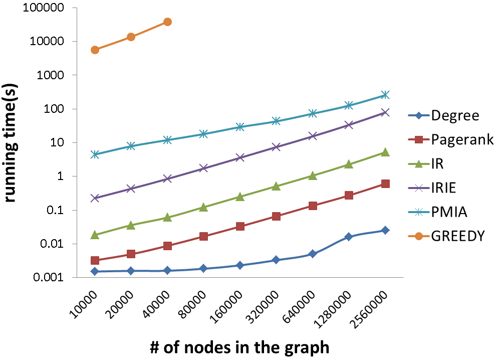
(a) Weighted Cascade

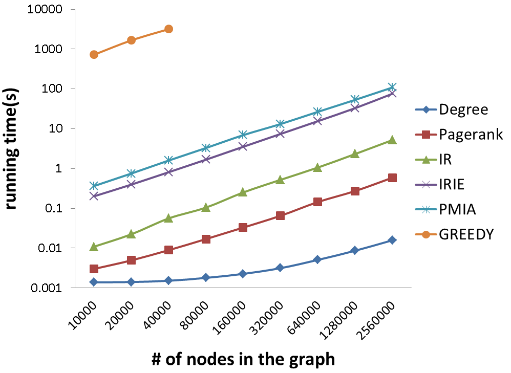
(b) Trivalency

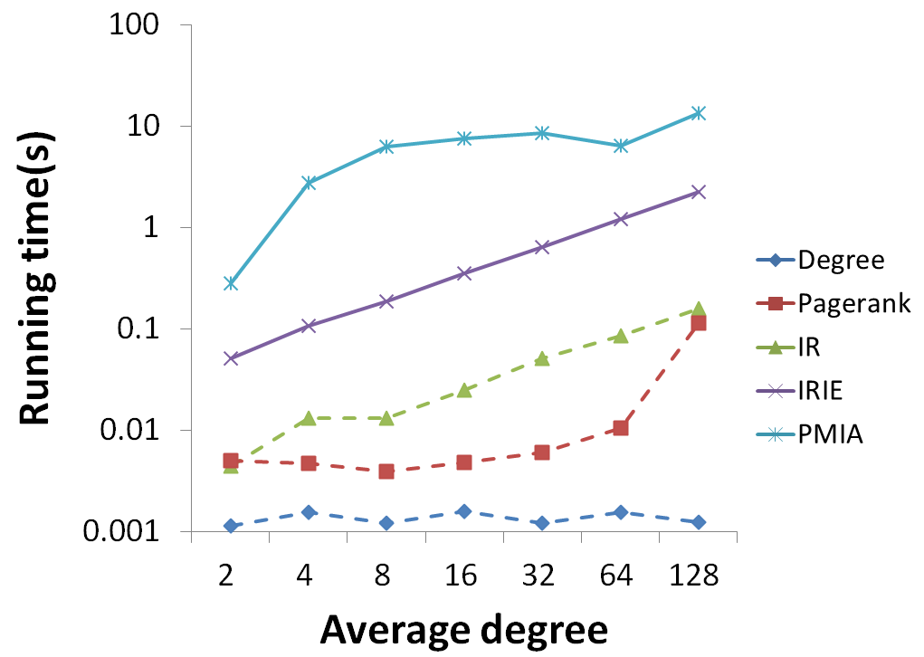
(c) Weighted Cascade

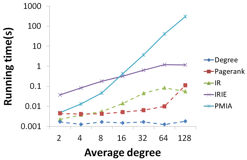
(d) Trivalency

Figure 4.1: Scalability test for the synthetic dataset

We compare our algorithms with state-of-the-art algorithms. The list of algorithms and corresponding parameter settings are as follows.

Degree A baseline algorithm selecting $K$ seed nodes with highest degree.

PageRank A baseline algorithm selecting $K$ seed nodes with highest ranking according to a diffusion process. In our experiments, we used the following weighted version of PageRank [3]. The transition probability $TP_{uv}$ along edge $(u,v)$ is defined by $TP_{uv}=P_{vu}/\sum_{w\in N^{in}(u)}P_{wu}$. The more activation probability along the edge $(u,v)$, the more transition probability of moving from $u$ to $v$. We set the random jump factor of PageRank as 0.15 as in [3].

CELF Greedy algorithm with Cost-Effective Lazy Forward(CELF) optimization [13].

SAEDV Simulated Annealing with Effective Diffusion Values(SAEDV) [9] uses an efficient heuristic measure to estimate influence of a set of nodes, which significantly running time of the algorithm. We do simulations with the proposed parameter settings, as well as our tuned parameters for our datasets. In our tuned parameters, we set initial temperature $T_{0}=5|V|$. The parameters $q$ and $\bigtriangleup T$ are set as 1000 and 2000 respectively as in [9]. We use the down-hill probability to be $exp\left(\frac{\bigtriangleup f\cdot C_{i}}{\sqrt{T_{t}}}\right)$ where $C_{i}$ is the number of iterations. We present results with better accuracy among the original parameters and our tuned parameters for each dataset.

PMIA PMIA [3] restricts the influence estimation for a set of nodes on local shortest-paths. The parameter $\theta$ of PMIA is set to 1/320 as in [3].

IR Our Algorithm 3 with $\alpha=0.7$.

IRIE Our Algorithm 4 with $\alpha=0.7$. Another parameter $\theta$ for generating MIOA [3] is set to 1/320 as in [3].

As the stopping criteria of IR and IRIE, we use the followings. For IR and the first round of IRIE, i.e., when $S=\emptyset$, we stop iterative computations for corresponding formulas when for each $u\in V$, difference between current $r(u)$ and the previous $r(u)$ is less than $0.0001$. Otherwise iterative computations run 20 rounds. For the subsequent rounds of IRIE, we initialize each $r(u)$ by the output of the previous round. Since those initial values make the iteration converge much faster, we run the iterations of line 10-12 of Algorithm 4 at most 5 times and apply the same stopping criteria as in the first round.

Algorithms for IC-N Model.

CELF-N Greedy algorithm with cost-effective lazy forward optimization [13] with the influence function $\sigma_{G}(S,q)$.

MIA-N MIA-N proposed in [2] is a variation of PMIA for IC-N model. The parameter $\theta$ of MIA-N is set to 1/160 as in [2].

IRIE-N Our Algorithm 5 with $\alpha$ = 0.7. We set the parameter $\theta$ for generating MIOA [3] as 1/160. The same stopping criteria as in IRIE is used for IRIE-N.

To compare the amount of influence spread of above algorithms, we run the Monte-Carlo simulation on both IC and IC-N models 10,000 times for each seed set and take the average of the influence spreads. Our experimental environment is a server with 2.8GHZ Quad-Core Intel i7 930 and 24GB memory.

4.2 Experimental Results

4.2.1 Scalability Test for the Synthetic Dataset

Figure 4.1 shows the experimental results on scalability of the algorithms. For Figures 4.1(a) and 4.1(b), we generate synthetic power-law random network datasets by increasing the number of nodes $|V|$ = 2K, 4K, 8K, …, 256K while fixing the average degree = 10. For Figures 4.1(c) and 4.1(d), we generate second synthetic power-law networks by fixing $|V|=2K$ and increasing the number of edges $|E|$ = 2K, 4K, …, 128K. We set $K=50$, and the figures are plotted in log-log scale. In Figures 4.1(a) and 4.1(b), IR and IRIE  show efficient running time and scalability. PMIA is also scalable in the number of nodes but about 2-10 times slower than IR and IRIE. In 4.1(c) and 4.1(d), IR and IRIE shows much better running time and scalability over the average degree than PMIA. Hence we find that IR and IRIE show much more robust performance over the edge density than PMIA in terms of scalability.

4.2.2 Sensitivity to Propagation Probability Models

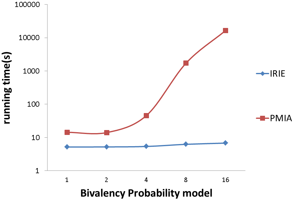
Figure 4.1: Sensitivity of algorithms under various Bivalency models for the Epinions dataset

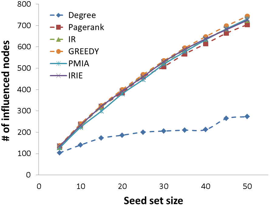
(a) Arxiv-WC

(b) Arxiv-TR

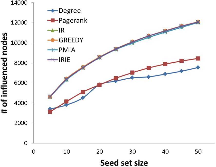
(c) Epinions-WC

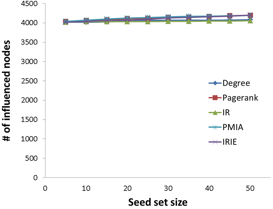
(d) Epinions-TR

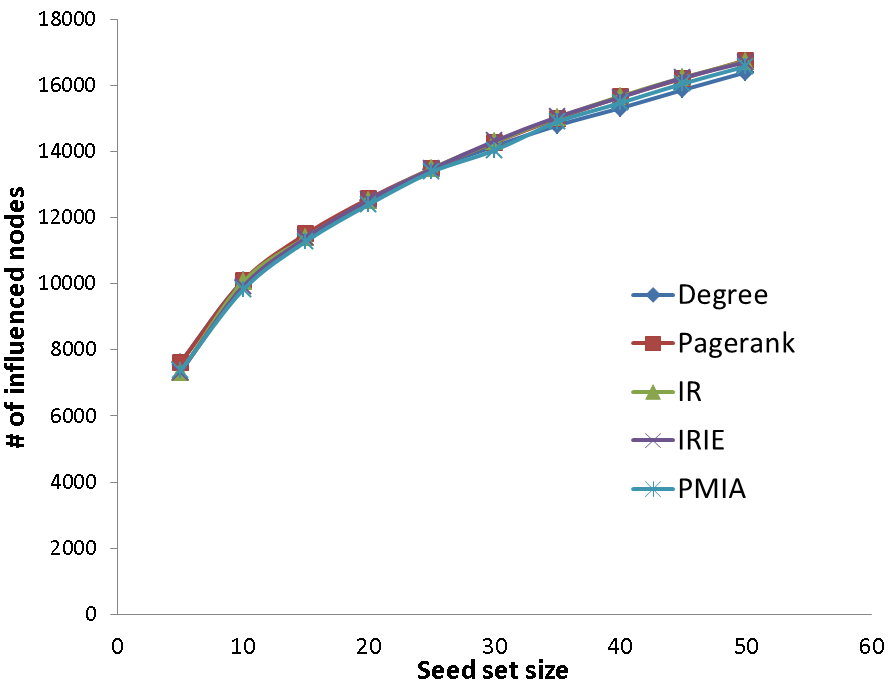
(e) Slashdot-WC

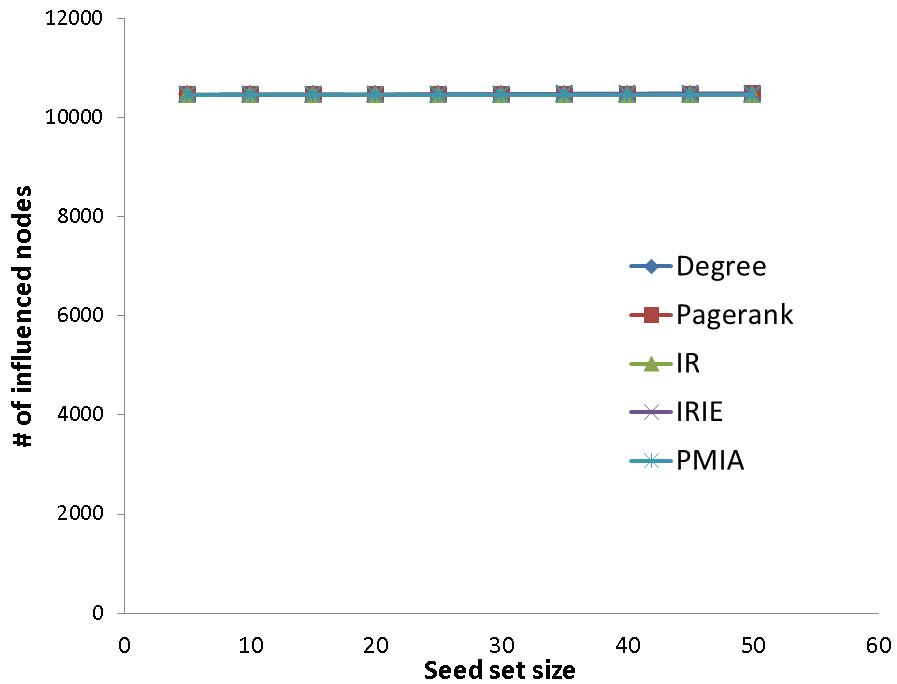
(f) Slashdot-TR

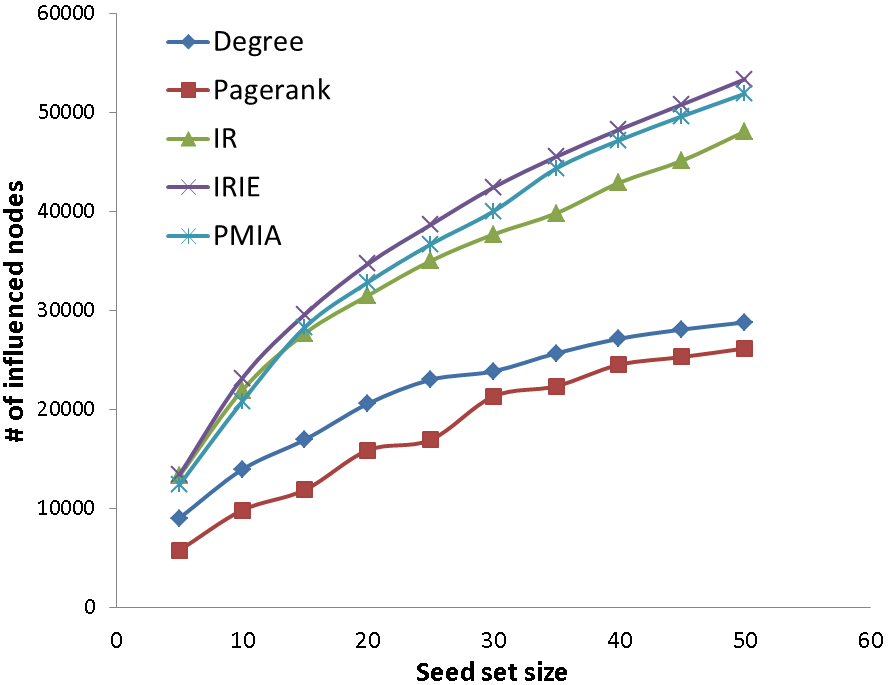
(g) DBLP-WC

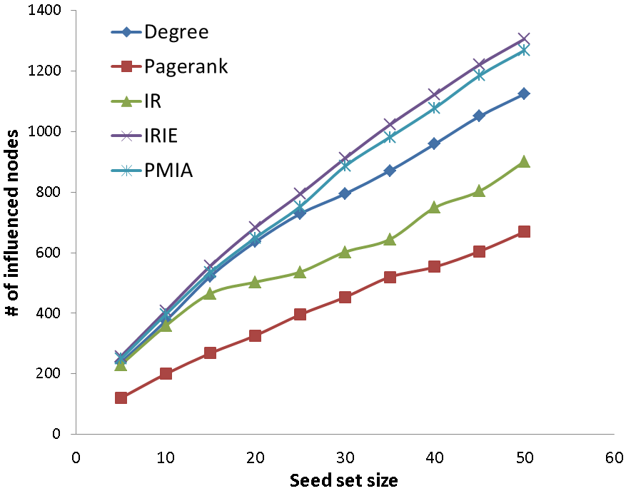
(h) DBLP-TR

Figure 4.1: Influence spreads for IC model

We compare IRIE with PMIA in terms of the sensitivity of running time to propagation probability models. In this experiment, we compare running times of IRIE and PMIA on Epinions dataset for various bivalency models described as follows. For each propagation model indexed by $i\in\{1,2,4,8,16\}$, edge propagation probabilities are randomly assigned from $i~{}\times~{}\{0.01,0.001\}$. We set the seed size $K=50$. In Figure 4.1, IRIE shows much faster and more stable running time than PMIA. The running time of IRIE slightly increases as the edge probability increases, while the running time of PMIA increases dramatically around $i=8$, where the spread size becomes large. Especially, IRIE is more than 1000 times faster than PMIA for the (0.16, 0.016)-bivalency model. Hence we observe that while the running time of PMIA is quite dependent on the spread size and the propagation model, the running time of IRIE  is very stable over them.

4.2.3 Influence Spread for the Real-World Datasets

We compare influence spread for each algorithms on the five real-world datasets. The seed size $K$ is set from 1 to 50 to compare the accuracies of algorithm in various range of seed sizes. Figure 4.1 (a)-(h) and Table 2 show the experimental results on influence spread. We run the CELF only for Arxiv, and Epinions(for the WC) since CELF runs too long for other datasets. We did Monte-Carlo simulation for LiveJournal only for $K$=50 since it takes too long time.

In general, CELF performs almost the best influence spread for both the WC and the TR models. However, IRIE shows almost similar performance with CELF in all cases. PMIA also shows high performance but 1-5% less influence spread than IRIE for all cases except for the Epinions TR. IR shows high performances for the WC models, but not quite good in the TR models. Hence we observe that IE part of IRIE is necessary to achieve robust performance in various steps. The baseline algorithms Degree and PageRank show low Performances for many cases such as Arxiv, Epinions, and DBLP. Unlike the Greedy based approaches, SAEDV computes the seed set for each $K$ independently.

Table 2: Influence spread at 50-seed set for LiveJournal

Algorithm	Weighted Cascade	Trivalency
IRIE	74830.5	629694
IR	75861.2	629484
PMIA	71566.5	629512
PageRank	51162.6	629892
Degree	52162.3	629498

Table 3: Influence spread at 50-seed set of SAEDV and IRIE

	WC		TR
Dataset	SAEDV	IRIE	SAEDV	IRIE
ArXiv	669.755	724.666	185.369	190.006
Epinions	11177.3	12063	4176.35	4200.22
Slashdot	14803	16712.3	10467.7	10490.2
Amazon	487.671	824.795	79.5405	82.041
DBLP	33730	53334.8	1175.53	1304.81

Hence we include Table 3 that shows the influence spread comparison of SAEDV with IRIE for $K$=50. Table 3 clearly shows that IRIE outperforms SAEDV in terms of influence spread by large margin for most cases. Hence we conclude that IRIE shows very high accuracy and robustness in most environments.

4.2.4 Running Time and Memory Usage for the Real-World Datasets

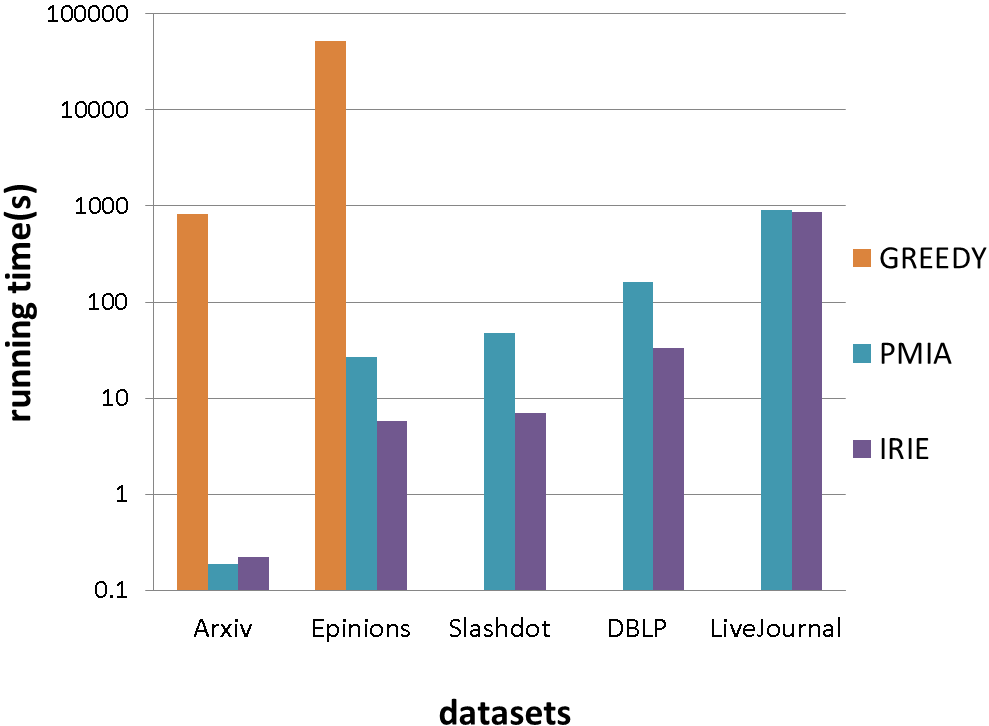
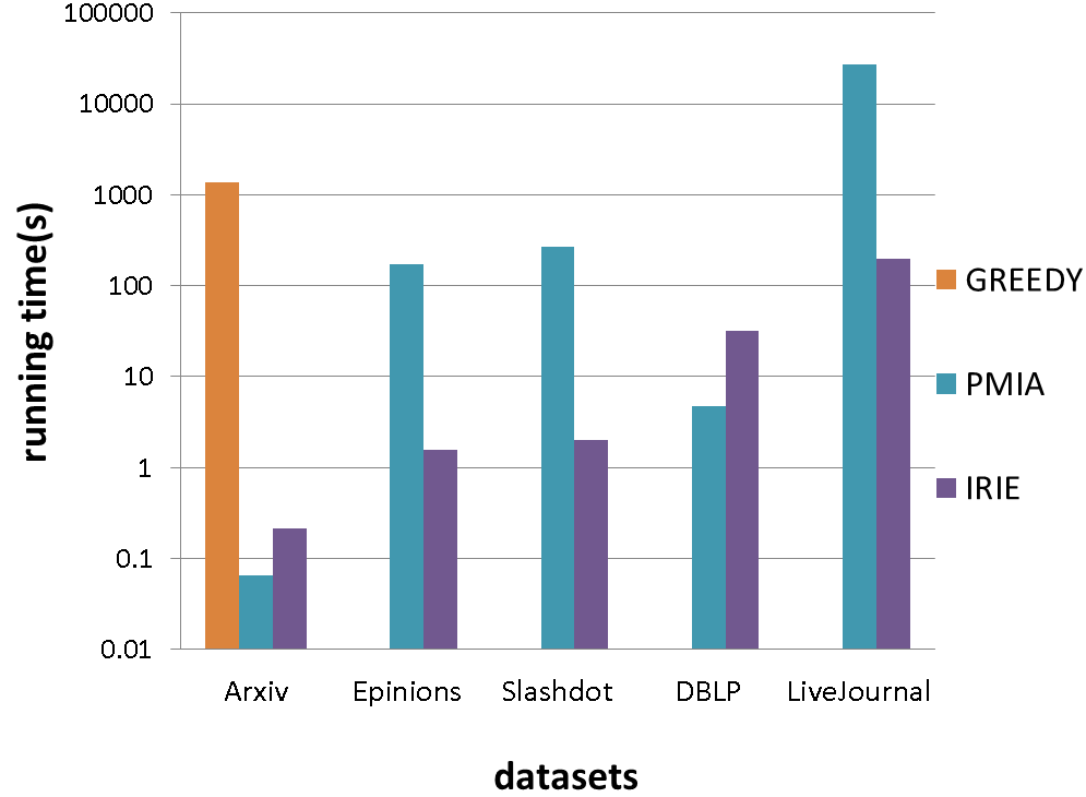
Figure 4.1: Running time of algorithms under IC model

Table 4: Memory usages of IRIE and PMIA

	WC			TR
Dataset	File size	PMIA	IRIE	File size	PMIA	IRIE
ArXiv	715KB	14MB	8.7MB	582KB	10MB	8.7MB
Epinions	18MB	135MB	35MB	15MB	143MB	35MB
Slashdot	24MB	280MB	39MB	19MB	340MB	40MB
DBLP	88MB	1.1GB	160MB	82MB	357MB	158MB
LiveJournal	2.4GB	10.1GB	3GB	2GB	16GB	3GB

We also checked the running time of the algorithms on the real-world social networks. Figure 4.1 shows the results. The left and right figures in 4.1 corresponds to the WC model and the TR model respectively. In each figure, datasets are aligned in increasing order of network sizes from left to right. For both the WC and the TR model, IRIE is more than 1000 times faster than the CELF. Also in most cases, IRIE is quite faster than PMIA. Note that the running time of IRIE is increasing as the dataset size increases from Arxiv to LiveJournal. However, the running times of PMIA are somewhat unstable, resulting in longer running times even in smaller graph in both the numbers of nodes and edges.

Note that although the numbers of nodes and edges of Epinions and Slashdot are smaller than those of DBLP, the running times of PMIA for Epinions and Slashdot are much larger than for DBLP. One possible explanation is that the running time of PMIA is sensitive to structural properties of the network such as the clustering coefficient (Epinions and Slashdot are social network dataset which contains many triangles) and edge density, and the spread size (note that Epinions TR and Slashdot TR induce larger spread than DBLP TR) which matches the results of the scalability test and the sensitivity test in Sections 4.2.1 and 4.2.2. Hence, we conclude that IRIE shows much more stable and faster running time than PMIA in various networks.

Table 4 shows the experimental results on the amount of memory used by algorithms for the WC and the TR model respectively. In the table, file sizes indicate the size of raw text data files, and PMIA and IRIE indicate the amount of memory occupied by corresponding algorithms. For the WC model, IRIE is much more efficient in terms of memory than PMIA for all the datasets. The memory usages of PMIA are 4-20 times larger than the size of raw data file and also 2-7 times larger than that of IRIE. Especially, for the LiveJournal dataset, PMIA requires about 10GB of memory spaces while IRIE requires only 3GB of memory which is close to the size of the raw text file. We observe the similar patterns in memory usage for the TR model. However, the amounts of memory occupied by PMIA are even larger than the WC model while the memory usages of IRIE are almost same with those for the WC model. For the LiveJournal, PMIA requires about 16GB of memory which is an infeasibly large amount of memory.

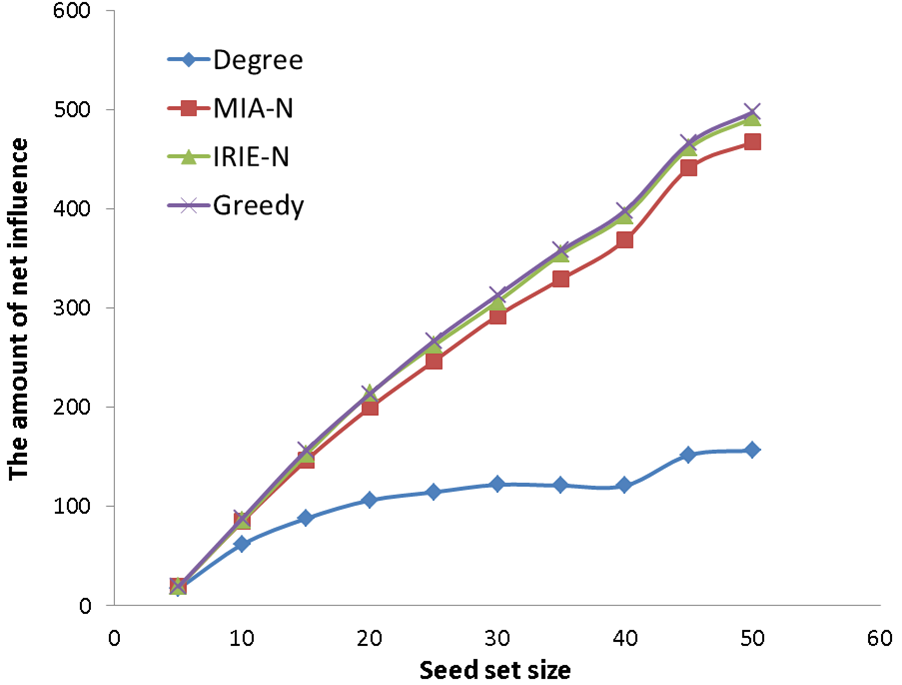
(a) Arxiv-WC

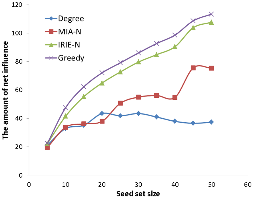
(b) Arxiv-TR

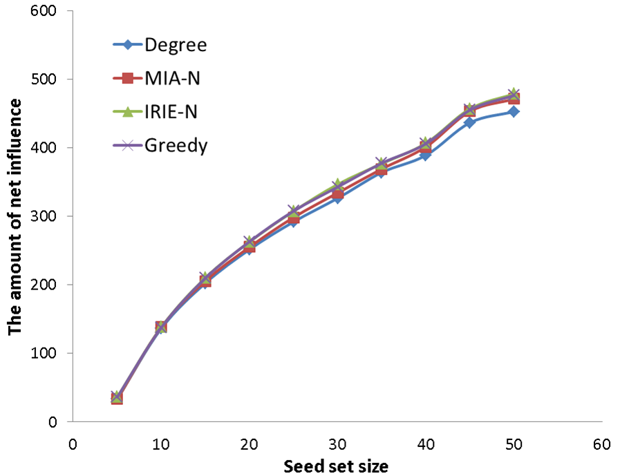
(c) Wiki-WC

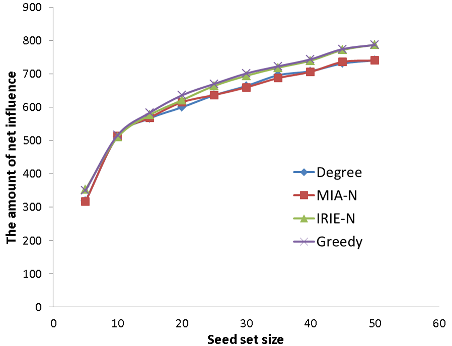
(d) Wiki-TR

Figure 4.1: Influence spreads for IC-N model with q = 0.9, $\lambda$ = 0

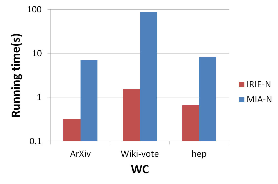
Figure 4.1: Running time of algorithms under IC-N model where q = 0.9, $\lambda$ = 0

4.3 Experiments on IC-N Model

In this subsection, we show experimental results for the IC-N model. Figure 4.1 (a)-(d) show the influence spread of the algorithms. When $\lambda=0$, Greedy-N and IRIE-N shows the best performances, while MIA-N shows slightly less performance than IRIE-N. Note that for Arxiv-TR, IRIE-N shows more stable influence spread than MIA-N. For the running time described in Figure 4.1, IRIE-N is about 5-50 times faster than MIA-N. Hence we conclude that IRIE-N is much faster than other algorithms while achieving best influence spread.

5 Conclusion

In this paper, we propose a new scalable and robust algorithm IRIE for influence maximization under the independent cascade (IC) model and its extension IC-N model. The IRIE algorithm incorporates fast iterative ranking algorithm (IR) with a fast influence estimation (IE) method to achieve scalability and robustness while maintaining good influence coverage. Comparing with other state-of-the-art influence maximization algorithms, the advantage of IRIE is that it avoids the storage and computation of local data structures, which results in significant savings in both memory usage and running time. Our extensive simulations results on synthetic and real-world networks demonstrate that IRIE is the best in influence coverage among all tested heuristics including PMIA, SAEDV, PageRank, degree heuristic, etc., and it achieves up to two orders of magnitude speed-up with only a small fraction of memory usage, especially on relatively dense social networks (with average degree greater than $10$), comparing with other state-of-the-art heuristics.

An additional advantage of IRIE is that its simple iterative computation can be readily ported to a parallel graph computation platform (e.g. Google’s Pregel [14]) to further scale up influence maximization, while other heuristics such as PMIA involves more complicated data structures and is relative harder for parallel implementation. A future direction is thus validating and improving the IRIE algorithm on a parallel graph computation platform. Another future direction is to apply the IRIE framework to other influence diffusion models, such as the linear threshold model.

Appendix

Appendix A Proof of Theorem 2

Proof.

First, note that Algorithm 2 computes the unique solution of (1) and (2). Let $m_{t}(u,v)$ be the expected number of activated nodes when $S=\{u\}$ and $u$ activates other nodes within distance $t$ from $u$ using all out-going edges of $u$ except for $(u,v)$. Let $\tilde{m}_{t}(u,v)$ be the computed values from Algorithm 2. Then we will prove that $\tilde{m}_{t}(u,v)=m_{t}(u,v)$ for all $t=0,1,2,\ldots$ by a mathematical induction. When $t=0$, $\tilde{m}_{0}(u,v)=m_{0}(u,v)=0$ for each edge $(v,u)\in E$.

Suppose that the statement is true for all $t<T$. Let $t=T$, and fix $u\in V$. Let $T_{u}$ be the tree graph $G$ whose root is $u$, and for each $w\in N^{out}(u)$, let $T_{uw}$ be the subtree of $T_{u}$ whose root is $w$. Note that $m_{t-1}(w,u)$ is the expected influence of $\{w\}$ to the nodes in $T_{uw}$ within distance $t-1$ from $w$.

Since $T_{u}$ is a tree graph, by the linearity of expectation and the definition of $m_{t}(u,v)$, we have for any $(v,u)\in E$,

$$m(u,v)=1+\left(\sum_{w\in N^{out}(u),w\neq v}P_{uw}\cdot m(w,u)\right).$$ (13)

From the line 7 of Algorithm 2, for any $(v,u)\in E$,

$$\tilde{m}_{t}(u,v)=1+\left(\sum_{w\in N^{out}(u),w\neq v}P_{uw}\cdot\tilde{m}_{t-1}(w,u)\right).$$ (14)

From the induction hypothesis, $\tilde{m}_{t}(w,u)=m_{t-1}(w,u)$. Hence, from (13) and (14), we have that for any $(v,u)\in E$, $m_{t}(u,v)=\tilde{m}_{t}(u,v)$. Therefore we have shown the induction. Note that $m(u,v)=m_{|V|-1}(u,v)$ since the longest shortest path of $G$ has length at most $|V|-1$. Hence $\{m_{t}(u,v)\}_{t}$ converges before $t\leq|V|$, and the same holds for $\{\tilde{m}_{t}(u,v)\}_{t}$.

Since $\{\tilde{m}_{t}(u,v)\}$ are the converged values $\{\tilde{m}_{t}(u,v)\}_{t}$ by the line 7 of Algorithm 2, we have that $\tilde{m}(u,v)=\tilde{m}_{|V|}(u,v)=m_{|V|}(u,v)=m(u,v)$ for all $(v,u)\in E$.

Since $G$ is a tree, from the definition of $\sigma(u)$ and the linearity of expectation,

$$\sigma(u)=1+\sum_{v\in N^{out}(u)}P_{uv}\cdot m(v,u).$$

Here from (1), $\tilde{\sigma}(u)=\sigma(u)$ for all $u\in V$. ∎

References

- [1] S. Brin and L. Page. The anatomy of a large-scale hypertextual web search engine. Computer Networks, 1998.
- [2] W. Chen, A. Collins, R. Cummings, T. Ke, Z. Liu, D. Rincon, X. Sun, Y. Wang, W. Wei, and W. Yuan. Influence maximization in social networks when negative opinions may emerge and propagate. In SDM, 2011.
- [3] W. Chen, C. Wang, and Y. Wang. Scalable influence maximization for prevalent viral marketing in large-scale social networks. In KDD, 2010.
- [4] W. Chen, Y. Wang, , and S. Yang. Efficient influence maximization in social networks. In KDD, 2009.
- [5] W. Chen, Y. Yuan, and L. Zhang. Scalable influence maximization in social networks under the linear threshold model. In ICDM, 2010.
- [6] P. Domingos and M. Richardson. Mining the network value of customers. In KDD, 2001.
- [7] A. Goyal, F. Bonchi, and L. V. S. Lakshmanan. A data-based approach to social influence maximization. In PVLDB, 2011.
- [8] A. Goyal, W. Lu, and L. V. S. Lakshmanan. Celf++: optimizing the greedy algorithm for influence maximization in social networks. In WWW(Companion Volume), 2011.
- [9] Q. Jiang, G. Song, G. Cong, Y. Wang, W. Si, and K. Xie. Simulated annealing based influence maximization in social networks. In AAAI, 2011.
- [10] D. Kempe, J. Kleinberg, and E. Tardos. Maximizing the spread of influence through a social network. In KDD, 2003.
- [11] M. Kimura and K. Saito. Tractable models for information diffusion in social networks. In PKDD, pages 259–271. LNAI 4213, 2006.
- [12] J. Leskovec. http://snap.stanford.edu/index.html.
- [13] J. Leskovec, A. Krause, C. Guestrin, C. Faloutsos, J. VanBriesen, and N. S. Glance. Cost-effective outbreak detection in networks. In KDD, 2007.
- [14] G. Malewicz, M. H. Austern, A. J. C. Bik, J. C. Dehnert, I. Horn, N. Leiser, and G. Czajkowski. Pregel: a system for large-scale graph processing. In SIGMOD, 2010.
- [15] R. Narayanam and Y. Narahari. A shapley value based approach to discover influential nodes in social networks. IEEE Transactions on Automation Science and Engineering, 2010.
- [16] P. Rozin and E. B. Royzman. Negativity bias, negativity dominance, and contagion. Personality and Social Psychology Review, 2001.
- [17] Y. Wang, G. Cong, G. Song, , and K. Xie. Community-based greedy algorithm for mining top-k influential nodes in mobile social networks. In KDD, 2010.