Neutrino propagation in noncommutative spacetimes

Abstract:

One-loop $\theta$-exact quantum corrections to the neutrino propagator are computed in noncommutative $\rm U_{\star}(1)$ gauge-theory based on Seiberg-Witten maps. Our closed form results show that the one-loop correction contains a hard $1/\epsilon$ UV divergence, as well as a logarithmic IR-divergent term of the type $\ln\sqrt{(\theta p)^{2}}$, thus considerably softening the usual UV/IR mixing phenomenon. We show that both of these problematic terms vanish for a certain choice of the noncommutative parameter $\theta$ which preserves unitarity. We find non-perturbative modifications of the neutrino dispersion relations which are assymptotically independent of the scale of noncommutativity in both the low and high energy limits and may allow superluminal propagation. Finally, we demonstrate how the prodigious freedom in Seiberg-Witten maps may be used to affect neutrino propagation in a profound way.

1 Introduction

The study of spacetime quantization has originally been motivated by major problems of physics at extremely-high energies, in particular the problems of renormalization and quantum gravity. Heisenberg-type spacetime uncertainty relations can effectively lead to a replacement of the continuum of points by finite size spacetime cells, thus providing a means by which to tame UV divergences. A branch of mathematics arising from these motivations has come to be known as noncommutative geometry. It is reasonable to expect that noncommutative (NC) field theory models can provide some guidance for a deeper understanding of the structure of spacetime at extremely-high energies. In fact, these NC models appear quite naturally in string theory [1]. The relevant scale of noncommutativity may very well be beyond direct experimental reach for the foreseeable future (except in certain theories with large extra dimensions). Nevertheless, non-perturbative effects can nevertheless lead to profound observable consequences for low energy physics. A famous example is UV/IR mixing. Another striking example is the running of the coupling constant of noncommutative U(1) gauge theory in the simple star($\star$)-product formalism [2]. The beta function

$$\beta(g^{2})=-\frac{1}{8\pi^{2}}\frac{22}{3}g^{4}N^{2}$$ (1)

of NC $\rm U(N)$ gauge theory is identical to that of ordinary $\rm SU(N)$ Yang-Mills theory for $N>1$, but in the noncommutative case it remains valid even for Abelian $N=1$ gauge theory. Hence the theory will suffer from asymptotic freedom [2, 3]. This result is manifestly independent of the scale of noncommutativity and thus remains valid even for vanishingly small (but non-zero) noncommutivity.

In a simple model of NC spacetime local coordinates $x^{\mu}$ are promoted to hermitian operators $\hat{x}^{\mu}$ satisfying spacetime noncommutative relations

$$[\hat{x}^{\mu},\hat{x}^{\nu}]=i\theta^{\mu\nu},$$ (2)

where $\theta^{\mu\nu}$ is real antisymmetric matrix of dimension $length^{2}$. The commutator (2) implies spacetime uncertainty relations

$$\Delta x^{\mu}\Delta x^{\nu}\geq\frac{1}{2}|\theta^{\mu\nu}|.$$ (3)

It is straight-forward to formulate field theories on such noncommutative spaces as a deformation of the ordinary field theories. The noncommutative deformation is implemented by replacing the usual pointwise product of a pair of fields $f(x)$ and $g(x)$ by a $\star$-product in the action:

$$f(x)g(x)\longrightarrow(f\star g)(x)=f(x)g(x)+{\cal O}(\theta,\partial f,\partial g).$$ (4)

The Moyal-Weyl $\star$-product is relevant for the case of a constant $\theta^{\mu\nu}$ and is defined as follows:

$$(f\star g)(x)=f(x)e^{\frac{i}{2}\overleftarrow{{\partial}_{\mu}}\,\theta^{\mu\nu}\,\overrightarrow{{\partial}_{\nu}}}g(x).$$ (5)

(The $\star$-product has also an alternative integral formulation, making its non-local character more transparent.) The operator commutation relation (2) is then realized by the star($\star$)-commutator

$$[\hat{x}^{\mu},\hat{x}^{\nu}]=[x^{\mu}\stackrel{{\scriptstyle\star}}{{,}}x^{\nu}]=i\theta^{\mu\nu}.$$ (6)

In analogy to the introduction of covariant derivatives in gauge field theory, the star-product can be promoted to a gauge-field dependent covariant star product. Together with a gauge-field dependent covariant integral measure this generally leads to a noncommutative gauge field theory based on so-called Seiberg-Witten (SW) maps [1] . The resulting type of noncommutative quantum field theory has been studied for quite some time.

In this construction the noncommutative fields are obtained via SW maps from the original commutative fields. It is important to note that there is typically some freedom in the choice of SW map and that there is no warranty that every change in the choice of SW map will lead to a physically equivalent theory: Deformation, like quantization, is usually not unique and different deformations can lead to physically inequivalent models. The deformed model is not uniquely fixed by its commutative classical (tree level) $\theta\to 0$ limit. Different SW maps can behave like different quantization procedures.

The perturbative quantization of noncommutative field theories was first proposed in a pioneering paper about fifteen years ago [4]. Since then considerable efforts have been devoted to this subject. However, despite some significant progress like the models in [5, 6, 7], a complete understanding of quantum loop corrections still remains in general a challenging open question. This fact is particularly true for the models constructed by using Seiberg-Witten map expansion since the map was for a long time expressed as an approximative expansion in the noncommutative parameter $\theta$ [8, 9, 10, 11, 12]. One loop quantum properties [13, 14, 15, 16, 17, 18, 19, 20, 21, 22, 23, 24, 25], as well as the related phenomenology [26, 27, 28, 29, 30, 31] of the $\theta$-expanded models, have also been investigated recently.

The tree and one-loop analysis of the minimal NCSM truncated to first order in $\theta$ [19, 20, 31], has shown that considerably different physical behavior can arise from different choices of the Seiberg-Witten map. Furthermore, an analysis of the photon two-point function in a $\theta$-expanded model up to all orders via SW map [14] reveals that the parameters that fix the choice of SW map are running coupling constants [15]. This again indicates physical differences among different SW map deformations.

Some results about closed-form solutions and/or alternative $\theta$-exact approaches, starting from exact solutions for the Seiberg-Witten map, have existed for quite some time [32, 33, 34, 35]. Quite recently, $\theta$-exact SW map expansions, in the framework of covariant noncommutative quantum gauge field theory [36], were applied in loop computation [37, 38, 39] and phenomenology [40, 41]. These more sophisticated theories differ quite drastically from their $\theta$-expanded cousins, as they introduce in general a nonstandard denominator $p\theta q$ into the loop integral. A few methods have been proposed so far to handle this problem: An expansion and re-summation with respect to $\theta$ in the loop integral allowed some progress in [37]; another approximative method which also looks promising is integration using parametric derivatives. In general however, obtaining result in a closed form still remains a challenging problem [38].

In this article we obtain a closed formula for the one-loop correction to the propagator of a massless neutrino (neutral fermion) in the adjoint representation of $\rm U_{\star}(1)$ gauge group [39]. In the evaluation we combine parameterizations of Schwinger, Feynman, and a (modified) HQET parameterization [42], which was developed originally for heavy quark effective theory (HQET). This model is relatively easy to handle since both the gauge field and the fermion Seiberg-Witten map can be defined using generalized star products. The model is interesting in its own right for both theory and phenomenology: Its unexpanded version features a fermion-boson number symmetry which can cancel the leading order ultraviolet/infrared (UV/IR) mixing [43]. The model was also considered as an example for tree level neutrino-photon coupling via noncommutativity [11, 12].

The radiative corrections that we obtain contain in general both a hard UV term and a logarithmic IR singularity. At a special value of the noncommutative parameter $\theta$, both singularities vanishes. Analyzing the poles of the resulting (finite) modified neutrino propagator reveals, depending on the energy regime, modes with either heavy masses or modes whose propagation depends on the preferred direction in space set by $\theta^{\mu\nu}$. In the low-energy regime we find modes propagating superluminaly. These properties present some previously unknown features of $\theta$-exact noncommutative quantum field theories (NCQFT).

The article is structured as follows: In the following section we describe the actions of two alternative models which differ with regard to the choice of SW map and we give the relevant Feynman rules. Section 3 is devoted to the computation of the one-loop neutrino self-energy. Nonequivalent divergences and corresponding dispersion relations for both actions are described. Asymptotic dispersion relations are given for the low-energy and the high-energy regimes. Section 4 is devoted to discussion and conclusions. Relevant computational details of the nontrivial loop-integrals are given in two appendixes.

2 Model

In setting up our models we adhear to the following principles of $\theta$-exact NCGFT:
(i) The main principles that we are implementing in the construction of all of our $\theta$-exact noncommutative models are: The standard field content and the commutative gauge symmetry as the fundamental symmetry of the theory are fixed.
(ii) In the construction of the noncommutative action, generically, electrically neutral matter fields will be promoted via (hybrid) Seiberg-Witten maps to noncommutative fields that couple to photons and transform in the adjoint representation of $\rm U_{\star}(1)$.
(iii) The different actions discussed in this paper are constructed by employing SW map freedom.
(iv) The inclusion of all gauge covariant coupling terms into these actions is a prerequisite for reasonable UV behavior.

2.1 Action

Taking the above into account we arrive at the following model of the SW map type noncommutative $\rm U_{\star}(1)$ gauge theory with a gauge field $A_{\mu}$ coupled to a massless neutral fermion $\Psi$ via a star-commutator [11, 12]

$$[A_{\mu}\stackrel{{\scriptstyle\star}}{{,}}\Psi]=A_{\mu}\star\Psi-\Psi\star A_{\mu}.$$ (7)

The action is defined in the usual way [11, 12, 38]

$$S=\int-\frac{1}{4}F^{\mu\nu}\star F_{\mu\nu}+i\bar{\Psi}\star\mathchoice{\ooalign{$\hfil\displaystyle\mkern 0.0mu/\hfil$\crcr$\displaystyle D$}}{\ooalign{$\hfil\textstyle\mkern 0.0mu/\hfil$\crcr$\textstyle D$}}{\ooalign{$\hfil\scriptstyle\mkern 0.0mu/\hfil$\crcr$\scriptstyle D$}}{\ooalign{$\hfil\scriptscriptstyle\mkern 0.0mu/\hfil$\crcr$\scriptscriptstyle D$}}\Psi\,,$$ (8)

with definitions of the noncommutative covariant derivative and field strength resembling the corresponding expressions of non-abelian Yang-Mills theory:

$$D_{\mu}\Psi=\partial_{\mu}\Psi-i[A_{\mu}\stackrel{{\scriptstyle\star}}{{,}}\Psi]\quad\mbox{and}\quad F_{\mu\nu}=\partial_{\mu}A_{\nu}-\partial_{\nu}A_{\mu}-i[A_{\mu}\stackrel{{\scriptstyle\star}}{{,}}A_{\nu}].$$

All the NC fields in this action are images of the corresponding commutative fields $a_{\mu}$ and $\psi$ under (hybrid) Seiberg-Witten maps. In the original work of Seiberg and Witten and majority of the subsequent applications, these maps are understood as power series of the noncommutativity parameter $\theta^{\mu\nu}$. Physically, this corresponds to an expansion in momenta and is valid only for low energy phenomena. Here we give an alternative point of view and employ an expansion in formal powers of the gauge field $a_{\mu}$ and hence in powers of the coupling constant $e$. At each order in $a_{\mu}$ we shall determine $\theta$-exact expressions. In the following we discuss the model construction for the massless case, and we shall set $e=1$. To restore the coupling constant one simply substitutes $a_{\mu}$ by $ea_{\mu}$ and then divides the gauge-field term in the Lagrangian by $e^{2}$.

Next step we expand the action in terms of the commutative fields $a_{\mu}$ and $\psi$ using the following SW map solution [38]

$$\begin{split}A_{\mu}&=\,a_{\mu}-\frac{1}{2}\theta^{\nu\rho}{a_{\nu}}\star_{2}(\partial_{\rho}a_{\mu}+f_{\rho\mu})+\mathcal{O}(a^{3}),\\ \Psi&=\psi-\theta^{\mu\nu}{a_{\mu}}\star_{2}{\partial_{\nu}}\psi+\frac{1}{2}\theta^{\mu\nu}\theta^{\rho\sigma}\bigg{\{}(a_{\rho}\star_{2}(\partial_{\sigma}a_{\mu}+f_{\sigma\mu}))\star_{2}{\partial_{\nu}}\psi+2a_{\mu}{\star_{2}}(\partial_{\nu}(a_{\rho}{\star_{2}}\partial_{\sigma}\psi))\\ &-a_{\mu}{\star_{2}}(\partial_{\rho}a_{\nu}{\star_{2}}\partial_{\sigma}\psi)-\big{[}a_{\rho}\partial_{\mu}\psi(\partial_{\nu}a_{\sigma}+f_{\nu\sigma})-\partial_{\rho}\partial_{\mu}\psi a_{\nu}a_{\sigma}\big{]}_{\star_{3}}\bigg{\}}+\mathcal{O}(a^{3})\psi.\end{split}$$ (9)

Here the two generalized star products

$$f(x)\star_{2}g(x)=\frac{\sin\frac{\partial_{1}\theta\partial_{2}}{2}}{\frac{\partial_{1}\theta\partial_{2}}{2}}f(x_{1})g(x_{2})\bigg{|}_{x_{1}=x_{2}=x}\,,$$ (10)

$$[f(x)g(x)h(x)]_{\star_{3}}=\bigg{[}\frac{\sin(\frac{\partial_{2}\theta\partial_{3}}{2})\sin(\frac{\partial_{1}\theta(\partial_{2}+\partial_{3})}{2})}{\frac{(\partial_{1}+\partial_{2})\theta\partial_{3}}{2}\frac{\partial_{1}\theta(\partial_{2}+\partial_{3})}{2}}+\{1\leftrightarrow 2\}\,\bigg{]}f(x_{1})g(x_{2})h(x_{3})\bigg{|}_{x_{i}=x}\,,$$ (11)

are symmetric in their arguments, but nonassociative. The resulting expansion in the coupling constant defines the one-photon-two-fermion, two-photon-two-fermion and three-photon vertices $\theta$-exactly.

The expansion of the action is straightforward using the SW map (9). The first nontrivial contribution in the gauge field expansion leads to the following photon self-interaction terms

$$\begin{split}S_{g}=&\int\;i\partial_{\mu}a_{\nu}\star[a^{\mu}\stackrel{{\scriptstyle\star}}{{,}}a^{\nu}]+\frac{1}{2}\partial_{\mu}\left(\theta^{\rho\sigma}a_{\rho}\star_{2}(\partial_{\sigma}a_{\nu}+f_{\sigma\nu})\right)\star f^{\mu\nu}+\mathcal{O}(a^{4}).\end{split}$$ (12)

The photon-fermion interaction up to 2-photon-2-fermion terms is derived using the first order gauge field and second order fermion field expansion

$$\begin{split}S_{f}&=\int\;\bar{\psi}\gamma^{\mu}[a_{\mu}\stackrel{{\scriptstyle\star}}{{,}}\psi]+i(\theta^{ij}\partial_{i}\bar{\psi}\star_{2}a_{j})\mathchoice{\ooalign{$\hfil\displaystyle\mkern 0.0mu/\hfil$\crcr$\displaystyle\partial$}}{\ooalign{$\hfil\textstyle\mkern 0.0mu/\hfil$\crcr$\textstyle\partial$}}{\ooalign{$\hfil\scriptstyle\mkern 0.0mu/\hfil$\crcr$\scriptstyle\partial$}}{\ooalign{$\hfil\scriptscriptstyle\mkern 0.0mu/\hfil$\crcr$\scriptscriptstyle\partial$}}\psi-i\bar{\psi}\star\mathchoice{\ooalign{$\hfil\displaystyle\mkern 0.0mu/\hfil$\crcr$\displaystyle\partial$}}{\ooalign{$\hfil\textstyle\mkern 0.0mu/\hfil$\crcr$\textstyle\partial$}}{\ooalign{$\hfil\scriptstyle\mkern 0.0mu/\hfil$\crcr$\scriptstyle\partial$}}{\ooalign{$\hfil\scriptscriptstyle\mkern 0.0mu/\hfil$\crcr$\scriptscriptstyle\partial$}}(\theta^{ij}a_{i}\star_{2}\partial_{j}\psi)+(\theta^{ij}\partial_{i}\bar{\psi}\star_{2}a_{j})\gamma^{\mu}[a_{\mu}\stackrel{{\scriptstyle\star}}{{,}}\psi]\\ &-\!\bar{\psi}\gamma^{\mu}[a_{\mu}\!\stackrel{{\scriptstyle\star}}{{,}}\!\theta^{ij}a_{i}\!\star_{2}\!\partial_{j}\psi]\!-\!\frac{1}{2}\bar{\psi}\gamma^{\mu}[\theta^{ij}a_{i}\!\star_{2}\!(\partial_{j}a_{\mu}\!+\!f_{j\mu})\!\stackrel{{\scriptstyle\star}}{{,}}\!\psi]\!-\!i(\theta^{ij}\partial_{i}\bar{\psi}\!\star_{2}\!a_{j})\mathchoice{\ooalign{$\hfil\displaystyle\mkern 0.0mu/\hfil$\crcr$\displaystyle\partial$}}{\ooalign{$\hfil\textstyle\mkern 0.0mu/\hfil$\crcr$\textstyle\partial$}}{\ooalign{$\hfil\scriptstyle\mkern 0.0mu/\hfil$\crcr$\scriptstyle\partial$}}{\ooalign{$\hfil\scriptscriptstyle\mkern 0.0mu/\hfil$\crcr$\scriptscriptstyle\partial$}}(\theta^{kl}a_{k}\!\star_{2}\!\partial_{l}\psi)\\ &+\frac{i}{2}\theta^{ij}\theta^{kl}\bigg{(}(a_{k}\star_{2}(\partial_{l}a_{i}+f_{li}))\star_{2}\partial_{j}\bar{\psi}+2a_{i}\star_{2}(\partial_{j}(a_{k}\star_{2}\partial_{l}\bar{\psi}))-a_{i}\star_{2}(\partial_{k}a_{j}\star_{2}\partial_{l}\bar{\psi})\\ &+\big{[}a_{i}\partial_{k}\bar{\psi}(\partial_{j}a_{l}+f_{jl})-\partial_{k}\partial_{i}\bar{\psi}a_{j}a_{l}\big{]}_{\star_{3}}\bigg{)}\mathchoice{\ooalign{$\hfil\displaystyle\mkern 0.0mu/\hfil$\crcr$\displaystyle\partial$}}{\ooalign{$\hfil\textstyle\mkern 0.0mu/\hfil$\crcr$\textstyle\partial$}}{\ooalign{$\hfil\scriptstyle\mkern 0.0mu/\hfil$\crcr$\scriptstyle\partial$}}{\ooalign{$\hfil\scriptscriptstyle\mkern 0.0mu/\hfil$\crcr$\scriptscriptstyle\partial$}}\psi+\frac{i}{2}\theta^{ij}\theta^{kl}\bar{\psi}\mathchoice{\ooalign{$\hfil\displaystyle\mkern 0.0mu/\hfil$\crcr$\displaystyle\partial$}}{\ooalign{$\hfil\textstyle\mkern 0.0mu/\hfil$\crcr$\textstyle\partial$}}{\ooalign{$\hfil\scriptstyle\mkern 0.0mu/\hfil$\crcr$\scriptstyle\partial$}}{\ooalign{$\hfil\scriptscriptstyle\mkern 0.0mu/\hfil$\crcr$\scriptscriptstyle\partial$}}\bigg{(}(a_{k}\star_{2}(\partial_{l}a_{i}+f_{li}))\star_{2}\partial_{j}\psi\\ &+\!2a_{i}\!\star_{2}\!(\partial_{j}(a_{k}\!\star_{2}\!\partial_{l}\psi))\!-\!a_{i}\!\star_{2}\!(\partial_{k}a_{j}\!\star_{2}\!\partial_{l}\psi)\!+\big{[}a_{i}\partial_{k}\psi(\partial_{j}a_{l}\!+\!f_{jl})\!-\!\partial_{k}\partial_{i}\psi a_{j}a_{l}\big{]}_{\star_{3}}\bigg{)}\\ &+\bar{\psi}\mathcal{O}(a^{3})\psi.\end{split}$$ (13)

It is important to note that the actions (12) and (13) for gauge and matter fields respectively, are nonlocal objects due to the presence of the non-local (generalized) star products $\star$, $\star_{2}$ and $\star_{3}$. The appearance of non-locality in the actions is expected to be reflected in corresponding quantum corrections to the neutrino propagator (2-point functions).

2.2 Feynman rules

From the interaction terms we read out the three vertices needed for one-loop two point-function computations [44]

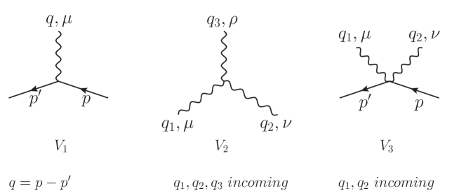
Figure 1: Three- and four-field vertices

$$V_{1}^{\mu}(q,p) = -F(q,p)[(q\theta p)\gamma^{\mu}+\mathchoice{\ooalign{$\hfil\displaystyle\mkern 0.0mu/\hfil$\crcr$\displaystyle p$}}{\ooalign{$\hfil\textstyle\mkern 0.0mu/\hfil$\crcr$\textstyle p$}}{\ooalign{$\hfil\scriptstyle\mkern 0.0mu/\hfil$\crcr$\scriptstyle p$}}{\ooalign{$\hfil\scriptscriptstyle\mkern 0.0mu/\hfil$\crcr$\scriptscriptstyle p$}}\tilde{q}^{\mu}-\mathchoice{\ooalign{$\hfil\displaystyle\mkern 0.0mu/\hfil$\crcr$\displaystyle q$}}{\ooalign{$\hfil\textstyle\mkern 0.0mu/\hfil$\crcr$\textstyle q$}}{\ooalign{$\hfil\scriptstyle\mkern 0.0mu/\hfil$\crcr$\scriptstyle q$}}{\ooalign{$\hfil\scriptscriptstyle\mkern 0.0mu/\hfil$\crcr$\scriptscriptstyle q$}}\tilde{p}^{\mu}],\;\;\;F(p,q)=\frac{\sin\frac{q\theta p}{2}}{\frac{q\theta p}{2}}\,,$$ (30)

$$V_{2}^{\mu\nu\rho}(q_{1},q_{2},q_{3})=-2\bigg{\{}\sin\frac{q_{1}\theta q_{2}}{2}[(q_{1}-q_{2})^{\rho}g^{\mu\nu}+(q_{2}-q_{3})^{\mu}g^{\nu\rho}+(q_{3}-q_{1})^{\nu}g^{\rho\mu}]$$ (31)

$$+ F(q_{1},q_{2})\Big{[}\theta^{\mu\nu}(q_{2}q_{3}q_{1}^{\rho}-q_{1}q_{3}q_{2}^{\rho})+\theta^{\mu\rho}(q_{2}q_{3}q_{1}^{\nu}-q_{1}q_{2}q_{3}^{\nu})+\theta^{\nu\rho}(q_{1}q_{3}q_{2}^{\mu}-q_{1}q_{2}q_{3}^{\mu})$$

$$- g^{\mu\nu}(q_{2}^{2}\tilde{q}_{1}^{\rho}+q_{1}^{2}\tilde{q}_{2}^{\rho})-g^{\mu\rho}(q_{1}^{2}\tilde{q}_{3}^{\nu}+q_{3}^{2}\tilde{q}_{1}^{\nu})-g^{\nu\rho}(q_{3}^{2}\tilde{q}_{2}^{\mu}+q_{2}^{2}\tilde{q}_{3}^{\mu})$$

$$+ q_{3}^{\rho}(\tilde{q}_{2}^{\mu}q_{3}^{\nu}+\tilde{q}_{1}^{\nu}q_{3}^{\mu})+q_{2}^{\nu}(\tilde{q}_{1}^{\rho}q_{2}^{\mu}+\tilde{q}_{3}^{\mu}q_{2}^{\rho})+q_{1}^{\mu}(\tilde{q}_{2}^{\rho}q_{1}^{\nu}+\tilde{q}_{3}^{\nu}q_{1}^{\rho})\Big{]}\bigg{\}}\,,$$

$$V^{\mu\nu}_{3}(q_{1},q_{2},p,p^{\prime})=2i\bigg{\{}2\frac{\sin\frac{q_{1}\theta p}{2}\sin\frac{q_{2}\theta p^{\prime}}{2}}{q_{1}\theta p}\tilde{p}^{\mu}\gamma^{\nu}-2i\frac{\sin\frac{q_{1}\theta p}{2}\sin\frac{q_{2}\theta p^{\prime}}{2}}{q_{2}\theta p^{\prime}}\tilde{p}^{{}^{\prime}\nu}\gamma^{\mu}$$ (56)

$$- \frac{\sin\frac{p\theta p^{\prime}}{2}\sin\frac{q_{1}\theta q_{2}}{2}}{q_{1}\theta q_{2}}(2\gamma^{\nu}\tilde{q}_{2}^{\mu}-\mathchoice{\ooalign{$\hfil\displaystyle\mkern 0.0mu/\hfil$\crcr$\displaystyle q$}}{\ooalign{$\hfil\textstyle\mkern 0.0mu/\hfil$\crcr$\textstyle q$}}{\ooalign{$\hfil\scriptstyle\mkern 0.0mu/\hfil$\crcr$\scriptstyle q$}}{\ooalign{$\hfil\scriptscriptstyle\mkern 0.0mu/\hfil$\crcr$\scriptscriptstyle q$}}_{2}\theta^{\mu\nu})-4i\frac{\sin\frac{q_{1}\theta p}{2}\sin\frac{q_{2}\theta p^{\prime}}{2}}{q_{1}\theta pq_{2}\theta p^{\prime}}(\mathchoice{\ooalign{$\hfil\displaystyle\mkern 0.0mu/\hfil$\crcr$\displaystyle q$}}{\ooalign{$\hfil\textstyle\mkern 0.0mu/\hfil$\crcr$\textstyle q$}}{\ooalign{$\hfil\scriptstyle\mkern 0.0mu/\hfil$\crcr$\scriptstyle q$}}{\ooalign{$\hfil\scriptscriptstyle\mkern 0.0mu/\hfil$\crcr$\scriptscriptstyle q$}}_{2}+\mathchoice{\ooalign{$\hfil\displaystyle\mkern 0.0mu/\hfil$\crcr$\displaystyle p$}}{\ooalign{$\hfil\textstyle\mkern 0.0mu/\hfil$\crcr$\textstyle p$}}{\ooalign{$\hfil\scriptstyle\mkern 0.0mu/\hfil$\crcr$\scriptstyle p$}}{\ooalign{$\hfil\scriptscriptstyle\mkern 0.0mu/\hfil$\crcr$\scriptscriptstyle p$}}^{\prime})\tilde{p}^{\mu}\tilde{p}^{{}^{\prime}\nu}$$

$$+ \mathchoice{\ooalign{$\hfil\displaystyle\mkern 0.0mu/\hfil$\crcr$\displaystyle p$}}{\ooalign{$\hfil\textstyle\mkern 0.0mu/\hfil$\crcr$\textstyle p$}}{\ooalign{$\hfil\scriptstyle\mkern 0.0mu/\hfil$\crcr$\scriptstyle p$}}{\ooalign{$\hfil\scriptscriptstyle\mkern 0.0mu/\hfil$\crcr$\scriptscriptstyle p$}}^{\prime}\bigg{[}\frac{\sin\frac{p\theta p^{\prime}}{2}\sin\frac{q_{1}\theta q_{2}}{2}}{q_{1}\theta q_{2}p\theta p^{\prime}}(q_{2}\theta p\theta^{\mu\nu}-2\tilde{q}_{2}^{\mu}\tilde{p}^{\nu})$$

$$- \frac{\sin\frac{q_{1}\theta p^{\prime}}{2}\sin\frac{q_{2}\theta p}{2}}{p_{1}\theta p^{\prime}q_{2}\theta p}2(\tilde{q}_{2}-\tilde{p})^{\mu}\tilde{p}^{\nu}+\frac{\sin\frac{q_{1}\theta p^{\prime}}{2}\sin\frac{q_{2}\theta p}{2}}{q_{1}\theta p}\theta^{\mu\nu}$$

$$+ \bigg{(}\frac{\sin\frac{q_{2}\theta p}{2}\sin\frac{q_{1}\theta p^{\prime}}{2}}{q_{2}\theta p^{\prime}q_{1}\theta p^{\prime}}+\frac{\sin\frac{q_{1}\theta q_{2}}{2}\sin\frac{p\theta p^{\prime}}{2}}{q_{2}\theta p^{\prime}p\theta p^{\prime}}\bigg{)}(2\tilde{p}^{\nu}\tilde{q}_{2}^{\mu}+\theta^{\mu\nu}p\theta q_{2}-\tilde{p}^{\mu}\tilde{p}^{\nu})\bigg{]}$$

$$+ \mathchoice{\ooalign{$\hfil\displaystyle\mkern 0.0mu/\hfil$\crcr$\displaystyle p$}}{\ooalign{$\hfil\textstyle\mkern 0.0mu/\hfil$\crcr$\textstyle p$}}{\ooalign{$\hfil\scriptstyle\mkern 0.0mu/\hfil$\crcr$\scriptstyle p$}}{\ooalign{$\hfil\scriptscriptstyle\mkern 0.0mu/\hfil$\crcr$\scriptscriptstyle p$}}\bigg{[}\frac{\sin\frac{p^{\prime}\theta p}{2}\sin\frac{q_{1}\theta q_{2}}{2}}{q_{1}\theta q_{2}p^{\prime}\theta p}(2\tilde{q}_{2}^{\mu}\tilde{p}^{{}^{\prime}\nu}-q_{2}\theta p^{\prime}\theta^{\mu\nu})$$

$$+ \frac{\sin\frac{q_{1}\theta p}{2}\sin\frac{q_{2}\theta p^{\prime}}{2}}{q_{1}\theta pq_{2}\theta p^{\prime}}2(\tilde{q}_{2}+\tilde{p}^{\prime})^{\mu}\tilde{p}^{{}^{\prime}\nu}-\frac{\sin\frac{q_{1}\theta p}{2}\sin\frac{q_{2}\theta p^{\prime}}{2}}{q_{1}\theta p}\theta^{\mu\nu}$$

$$- \bigg{(}\frac{\sin\frac{q_{2}\theta p^{\prime}}{2}\sin\frac{q_{1}\theta p}{2}}{q_{2}\theta pp_{1}\theta p}+\frac{\sin\frac{q_{2}\theta q_{1}}{2}\sin\frac{p^{\prime}\theta p}{2}}{q_{2}\theta pp^{\prime}\theta p}\bigg{)}(2\tilde{p}^{{}^{\prime}\nu}\tilde{q}_{2}^{\mu}+\theta^{\mu\nu}p^{\prime}\theta q_{2}+\tilde{p}^{{}^{\prime}\mu}\tilde{p}^{{}^{\prime}\nu})\bigg{]}\bigg{\}}$$

$$+ \{q_{1}\leftrightarrow q_{2}\,\mbox{and}\,\mu\leftrightarrow\nu\}\,,$$ (75)

where ${\tilde{q}}^{\mu}=(\theta q)^{\mu}=\theta^{\mu\nu}q_{\nu}$, and in addition we define ${\tilde{\tilde{q}}}^{\mu}=(\theta\theta q)^{\mu}=\theta^{\mu\nu}\theta_{\nu\rho}q^{\rho}$ .

2.3 Alternative actions and Feynman rules

As discussed in [41], there exist alternative consistent and covariant choices for the noncommutative interactions. This is related to a freedom in the choice of SW maps used in the construction of the theory. For the action (13) and Feynman rules (30), (75) , we presented in this section an alternative construction of the massless action, with coupling constant $e=1$.

We start with the action for a neutral massless free fermion field

$$S_{f}=\int\bar{\psi}\gamma^{\mu}\partial_{\mu}\psi\,=\int\bar{\psi}\star\gamma^{\mu}\partial_{\mu}\psi\,\,,$$ (76)

where, as indicated, a Moyal-Weyl type star product can be inserted or removed by partial integration. Following the method of constructing a covariant NC gauge theory outlined at the beginning of this section, we lift the factors in the action via (generalized) Seiberg-Witten maps $\hat{\Psi}[\bar{\psi},...]$, $\hat{\Phi}[\partial_{\mu}\psi,...]$ to noncommutative status as follows:

$$S_{f}\to S_{f_{alt}}=\int\hat{\Psi}(\bar{\psi})\gamma^{\mu}\hat{\Phi}(\partial_{\mu}\psi)\,=\int\hat{\Psi}(\bar{\psi})\star\gamma^{\mu}\hat{\Phi}(\partial_{\mu}\psi)\,\,.$$ (77)

Now if the SW maps $\hat{\Psi}$, $\hat{\Phi}$ and a corresponding map $\hat{\Lambda}$ for the gauge parameter $\lambda$ satisfy

$$\begin{split}\delta_{\lambda}(\hat{\Psi}(\bar{\psi}))=i[\hat{\Lambda}(\lambda)\stackrel{{\scriptstyle\star}}{{,}}\hat{\Psi}(\bar{\psi})],\\ \delta_{\lambda}(\hat{\Phi}(\partial_{\mu}\psi))=i[\hat{\Lambda}(\lambda)\stackrel{{\scriptstyle\star}}{{,}}\hat{\Phi}(\partial_{\mu}\psi)]\,,\end{split}$$ (78)

we will have a noncommutative action which is gauge invariant under infinitesimal commutative gauge transformations $\delta_{\lambda}$ and reduces to the free fermion action in the commutative limit $\theta\to 0$.

The appropriate map $\hat{\Psi}$ can be the same as in (9). Recalling that we are dealing with neutral fields, i.e. $\delta\psi=0$ and $\delta(\partial_{\mu}\psi)=0$, we notice that we can in principle use the same map also for $\hat{\Phi}$:

$$\begin{split}\hat{\Phi}_{alt2}(\partial_{\mu}\psi)&=\hat{\Psi}(\partial_{\mu}\psi)=\Psi(\psi\to\partial_{\mu}\psi)=\partial_{\mu}\psi-\theta^{ij}{a_{i}}\star_{2}\partial_{j}(\partial_{\mu}\psi)\\ &+\frac{1}{2}\theta^{ij}\theta^{kl}\bigg{\{}(a_{k}\star_{2}(\partial_{l}a_{i}+f_{li}))\star_{2}{\partial_{j}}(\partial_{\mu}\psi)+2a_{i}{\star_{2}}(\partial_{j}(a_{k}{\star_{2}}\partial_{l}(\partial_{\mu}\psi)))\\ &-a_{i}{\star_{2}}(\partial_{k}a_{j}{\star_{2}}\partial_{l}(\partial_{\mu}\psi))-\big{[}a_{k}\partial_{i}(\partial_{\mu}\psi)(\partial_{j}a_{l}+f_{jl})-\partial_{k}\partial_{i}(\partial_{\mu}\psi)a_{j}a_{l}\big{]}_{\star_{3}}\bigg{\}}+\mathcal{O}(a^{3})\psi\,.\end{split}$$ (79)

This construction is quite unusual from the point of gauge theory, as it yields a covariant derivative term without introducing a covariant derivative. In any case the resulting action

$$\begin{split}S_{f_{alt2}}=&\int\Big{(}i\bar{\psi}\mathchoice{\ooalign{$\hfil\displaystyle\mkern 0.0mu/\hfil$\crcr$\displaystyle\partial$}}{\ooalign{$\hfil\textstyle\mkern 0.0mu/\hfil$\crcr$\textstyle\partial$}}{\ooalign{$\hfil\scriptstyle\mkern 0.0mu/\hfil$\crcr$\scriptstyle\partial$}}{\ooalign{$\hfil\scriptscriptstyle\mkern 0.0mu/\hfil$\crcr$\scriptscriptstyle\partial$}}\psi-i\left(\theta^{ij}\partial_{j}\bar{\psi}\star_{2}a_{i}\right)\mathchoice{\ooalign{$\hfil\displaystyle\mkern 0.0mu/\hfil$\crcr$\displaystyle\partial$}}{\ooalign{$\hfil\textstyle\mkern 0.0mu/\hfil$\crcr$\textstyle\partial$}}{\ooalign{$\hfil\scriptstyle\mkern 0.0mu/\hfil$\crcr$\scriptstyle\partial$}}{\ooalign{$\hfil\scriptscriptstyle\mkern 0.0mu/\hfil$\crcr$\scriptscriptstyle\partial$}}\psi+i\bar{\psi}\left(\theta^{ij}a_{i}\star_{2}\mathchoice{\ooalign{$\hfil\displaystyle\mkern 0.0mu/\hfil$\crcr$\displaystyle\partial$}}{\ooalign{$\hfil\textstyle\mkern 0.0mu/\hfil$\crcr$\textstyle\partial$}}{\ooalign{$\hfil\scriptstyle\mkern 0.0mu/\hfil$\crcr$\scriptstyle\partial$}}{\ooalign{$\hfil\scriptscriptstyle\mkern 0.0mu/\hfil$\crcr$\scriptscriptstyle\partial$}}\partial_{j}\psi\right)\Big{)}\,\;\\ &+i\left(\theta^{ij}\partial_{j}\bar{\psi}\star_{2}a_{i}\right)(\theta^{kl}{a_{k}}\star_{2}\partial_{l}(\mathchoice{\ooalign{$\hfil\displaystyle\mkern 0.0mu/\hfil$\crcr$\displaystyle\partial$}}{\ooalign{$\hfil\textstyle\mkern 0.0mu/\hfil$\crcr$\textstyle\partial$}}{\ooalign{$\hfil\scriptstyle\mkern 0.0mu/\hfil$\crcr$\scriptstyle\partial$}}{\ooalign{$\hfil\scriptscriptstyle\mkern 0.0mu/\hfil$\crcr$\scriptscriptstyle\partial$}}\psi))\\ &-\frac{i}{2}\theta^{ij}\theta^{kl}\bigg{\{}(a_{k}\star_{2}(\partial_{l}a_{i}+f_{li}))\star_{2}{\partial_{j}}\bar{\psi}+2a_{i}{\star_{2}}(\partial_{j}(a_{k}{\star_{2}}\partial_{l}\bar{\psi}))\\ &-a_{i}{\star_{2}}(\partial_{k}a_{j}{\star_{2}}\bar{\psi})-\big{[}a_{k}\partial_{i}\bar{\psi}(\partial_{j}a_{l}+f_{jl})-\partial_{k}\partial_{i}(\bar{\psi})a_{j}a_{l}\big{]}_{\star_{3}}\bigg{\}}\mathchoice{\ooalign{$\hfil\displaystyle\mkern 0.0mu/\hfil$\crcr$\displaystyle\partial$}}{\ooalign{$\hfil\textstyle\mkern 0.0mu/\hfil$\crcr$\textstyle\partial$}}{\ooalign{$\hfil\scriptstyle\mkern 0.0mu/\hfil$\crcr$\scriptstyle\partial$}}{\ooalign{$\hfil\scriptscriptstyle\mkern 0.0mu/\hfil$\crcr$\scriptscriptstyle\partial$}}\psi\\ &+\frac{i}{2}\theta^{ij}\theta^{kl}\bar{\psi}\bigg{\{}(a_{k}\star_{2}(\partial_{l}a_{i}+f_{li}))\star_{2}{\partial_{j}}(\mathchoice{\ooalign{$\hfil\displaystyle\mkern 0.0mu/\hfil$\crcr$\displaystyle\partial$}}{\ooalign{$\hfil\textstyle\mkern 0.0mu/\hfil$\crcr$\textstyle\partial$}}{\ooalign{$\hfil\scriptstyle\mkern 0.0mu/\hfil$\crcr$\scriptstyle\partial$}}{\ooalign{$\hfil\scriptscriptstyle\mkern 0.0mu/\hfil$\crcr$\scriptscriptstyle\partial$}}\psi)+2a_{i}{\star_{2}}(\partial_{j}(a_{k}{\star_{2}}\partial_{l}(\mathchoice{\ooalign{$\hfil\displaystyle\mkern 0.0mu/\hfil$\crcr$\displaystyle\partial$}}{\ooalign{$\hfil\textstyle\mkern 0.0mu/\hfil$\crcr$\textstyle\partial$}}{\ooalign{$\hfil\scriptstyle\mkern 0.0mu/\hfil$\crcr$\scriptstyle\partial$}}{\ooalign{$\hfil\scriptscriptstyle\mkern 0.0mu/\hfil$\crcr$\scriptscriptstyle\partial$}}\psi)))\\ &-a_{i}{\star_{2}}(\partial_{k}a_{j}{\star_{2}}\partial_{l}(\mathchoice{\ooalign{$\hfil\displaystyle\mkern 0.0mu/\hfil$\crcr$\displaystyle\partial$}}{\ooalign{$\hfil\textstyle\mkern 0.0mu/\hfil$\crcr$\textstyle\partial$}}{\ooalign{$\hfil\scriptstyle\mkern 0.0mu/\hfil$\crcr$\scriptstyle\partial$}}{\ooalign{$\hfil\scriptscriptstyle\mkern 0.0mu/\hfil$\crcr$\scriptscriptstyle\partial$}}\psi))-\big{[}a_{k}\partial_{i}(\mathchoice{\ooalign{$\hfil\displaystyle\mkern 0.0mu/\hfil$\crcr$\displaystyle\partial$}}{\ooalign{$\hfil\textstyle\mkern 0.0mu/\hfil$\crcr$\textstyle\partial$}}{\ooalign{$\hfil\scriptstyle\mkern 0.0mu/\hfil$\crcr$\scriptstyle\partial$}}{\ooalign{$\hfil\scriptscriptstyle\mkern 0.0mu/\hfil$\crcr$\scriptscriptstyle\partial$}}\psi)(\partial_{j}a_{l}+f_{jl})-\partial_{k}\partial_{i}(\mathchoice{\ooalign{$\hfil\displaystyle\mkern 0.0mu/\hfil$\crcr$\displaystyle\partial$}}{\ooalign{$\hfil\textstyle\mkern 0.0mu/\hfil$\crcr$\textstyle\partial$}}{\ooalign{$\hfil\scriptstyle\mkern 0.0mu/\hfil$\crcr$\scriptstyle\partial$}}{\ooalign{$\hfil\scriptscriptstyle\mkern 0.0mu/\hfil$\crcr$\scriptscriptstyle\partial$}}\psi)a_{j}a_{l}\big{]}_{\star_{3}}\bigg{\}}\\ &+\mathcal{O}(a^{3})\,,\end{split}$$ (80)

is consistent and gauge invariant. The action leads to the following photon-fermion interaction vertices, i.e. Feynman rule,

$$V^{\mu}_{1_{alt2}}(q,p)=-F(q,p)(\theta q)^{\mu}\mathchoice{\ooalign{$\hfil\displaystyle\mkern 0.0mu/\hfil$\crcr$\displaystyle p$}}{\ooalign{$\hfil\textstyle\mkern 0.0mu/\hfil$\crcr$\textstyle p$}}{\ooalign{$\hfil\scriptstyle\mkern 0.0mu/\hfil$\crcr$\scriptstyle p$}}{\ooalign{$\hfil\scriptscriptstyle\mkern 0.0mu/\hfil$\crcr$\scriptscriptstyle p$}}\,,$$ (89)

$$V^{\mu\nu}_{3_{alt2}}(q_{1},q_{2},p,p^{\prime})=2i\mathchoice{\ooalign{$\hfil\displaystyle\mkern 0.0mu/\hfil$\crcr$\displaystyle p$}}{\ooalign{$\hfil\textstyle\mkern 0.0mu/\hfil$\crcr$\textstyle p$}}{\ooalign{$\hfil\scriptstyle\mkern 0.0mu/\hfil$\crcr$\scriptstyle p$}}{\ooalign{$\hfil\scriptscriptstyle\mkern 0.0mu/\hfil$\crcr$\scriptscriptstyle p$}}^{\prime}\bigg{\{}-2\frac{\sin\frac{q_{1}\theta p}{2}\sin\frac{q_{2}\theta p^{\prime}}{2}}{q_{1}\theta pq_{2}\theta p^{\prime}}\tilde{p}^{\mu}\tilde{p}^{{}^{\prime}\nu}$$ (98)

$$+\bigg{[}\frac{\sin\frac{p\theta p^{\prime}}{2}\sin\frac{q_{1}\theta q_{2}}{2}}{q_{1}\theta q_{2}p\theta p^{\prime}}(q_{2}\theta q_{1}\theta^{\mu\nu}-2\tilde{q}_{2}^{\mu}\tilde{p}^{\nu}+2\tilde{q}_{2}^{\mu}\tilde{p}^{{}^{\prime}\nu})$$

$$-\frac{\sin\frac{q_{1}\theta p^{\prime}}{2}\sin\frac{q_{2}\theta p}{2}}{q_{1}\theta p^{\prime}q_{2}\theta p}2(\tilde{q}_{2}-\tilde{p})^{\mu}\tilde{p}^{\nu}+\bigg{(}\frac{\sin\frac{q_{1}\theta p^{\prime}}{2}\sin\frac{q_{2}\theta p}{2}}{q_{1}\theta p^{\prime}}-\frac{\sin\frac{q_{1}\theta p}{2}\sin\frac{q_{2}\theta p^{\prime}}{2}}{q_{1}\theta p}\bigg{)}\theta^{\mu\nu}$$

$$+\bigg{(}\frac{\sin\frac{q_{2}\theta p}{2}\sin\frac{q_{1}\theta p^{\prime}}{2}}{q_{2}\theta p^{\prime}q_{1}\theta p^{\prime}}+\frac{\sin\frac{q_{1}\theta q_{2}}{2}\sin\frac{p\theta p^{\prime}}{2}}{q_{2}\theta p^{\prime}p\theta p^{\prime}}\bigg{)}(2\tilde{p}^{\nu}\tilde{q}_{2}^{\mu}+\theta^{\mu\nu}p\theta q_{2}-\tilde{p}^{\mu}\tilde{p}^{\nu})$$

$$+\frac{\sin\frac{q_{1}\theta p}{2}\sin\frac{q_{2}\theta p^{\prime}}{2}}{q_{1}\theta pq_{2}\theta p^{\prime}}2(\tilde{q}_{2}+\tilde{p}^{\prime})^{\mu}\tilde{p}^{\prime\nu}-\bigg{(}\frac{\sin\frac{q_{2}\theta p^{\prime}}{2}\sin\frac{q_{1}\theta p}{2}}{q_{2}\theta pq_{1}\theta p}+\frac{\sin\frac{q_{2}\theta p_{1}}{2}\sin\frac{p^{\prime}\theta p}{2}}{q_{2}\theta pp^{\prime}\theta p}\bigg{)}$$

$$\cdot(2\tilde{p}^{{}^{\prime}\nu}\tilde{q}_{2}^{\mu}+\theta^{\mu\nu}p^{\prime}\theta q_{2}+\tilde{p}^{{}^{\prime}\mu}\tilde{p}^{{}^{\prime}\nu})\bigg{]}\bigg{\}}+\{q_{1}\leftrightarrow q_{2}\,\mbox{and}\,\mu\leftrightarrow\nu\}\,.$$ (99)

There is also a second choice for $\hat{\Phi}$:

$$\hat{\Phi}_{alt3}(\partial_{\mu}\psi)=D_{\mu}\hat{\Psi}(\psi)\,.$$ (100)

This leads back to the original action discussed in the previous subsection. In general one can chose any superposition of the two SW maps $\hat{\Phi}_{alt2}$ and $\hat{\Phi}_{alt3}$ indicating a freedom in the choice of Seiberg-Witten map. Note that Feynman rule (30) is more natural from the point of view of gauge theory. In this article we analyze two different actions (Feynman rules), i.e. the original action and its alternative presented in this section. These essentially different actions (13) and (80), despite having the same field content and gauge symmetry, will be shown to produce different neutrino self-energies at one-loop in the next section.

Finally, the pure gauge field action $S_{g}$ in the alternative action, remains the same as in the original action. We keep $S_{g}$ and $V_{2}^{\mu\nu\rho}$ intact, that is we apply (31) in the computation of the two-point function from the alternative action.

3 One-loop neutrino self-energy

3.1 Diagrams

According to the vertices defined in the last section, there are four diagrams which contribute to the neutrino self-energy at one-loop

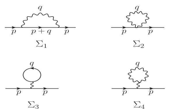
Figure 2: One-loop contributions to neutrino self-energy

$$\Sigma_{1-loop}=\Sigma_{1}+\Sigma_{2}+\Sigma_{3}+\Sigma_{4}\,$$ (101)

The first $\Sigma_{1}$ and third $\Sigma_{3}$ are the analog of the commutative fermion self-energy. The second one is similar to a tadpole graph in $\phi^{4}$ theory. However, it is not difficult to check, through direct computation from (75), that $g_{\mu\nu}V^{\mu\nu}_{3}(p,-p,q,q)=0$. Therefore $\Sigma_{2}$ is equal to zero. The last two diagrams, $\Sigma_{3}$ and $\Sigma_{4}$ are tadpole diagrams obtained by connecting a one-loop one-point function to a triple particle vertex. These two diagrams could be ruled out by the noncommutative charge conjugation symmetry defined in [10], so we do not take them into account. Namely, here we have taken the charge conjugation transformation to be the same as in the equations (64) to (66) from [10], i.e. ${\theta^{C}}^{\mu\nu}=-\theta^{\mu\nu}$. Thus only the two-point function bubble diagram $\Sigma_{1}$ needs to be evaluated.

3.2 Two-point function

The integral $\Sigma_{1}$ is defined as follows:

$$\Sigma_{1} = -\mu^{4-D}\int\frac{d^{D}q}{(2\pi)^{D}}\frac{-ig_{\alpha\beta}}{q^{2}}\cdot F(q,p)\left[(q\theta p)\gamma^{\alpha}+\mathchoice{\ooalign{$\hfil\displaystyle\mkern 0.0mu/\hfil$\crcr$\displaystyle p$}}{\ooalign{$\hfil\textstyle\mkern 0.0mu/\hfil$\crcr$\textstyle p$}}{\ooalign{$\hfil\scriptstyle\mkern 0.0mu/\hfil$\crcr$\scriptstyle p$}}{\ooalign{$\hfil\scriptscriptstyle\mkern 0.0mu/\hfil$\crcr$\scriptscriptstyle p$}}\tilde{q}^{\alpha}-\mathchoice{\ooalign{$\hfil\displaystyle\mkern 0.0mu/\hfil$\crcr$\displaystyle q$}}{\ooalign{$\hfil\textstyle\mkern 0.0mu/\hfil$\crcr$\textstyle q$}}{\ooalign{$\hfil\scriptstyle\mkern 0.0mu/\hfil$\crcr$\scriptstyle q$}}{\ooalign{$\hfil\scriptscriptstyle\mkern 0.0mu/\hfil$\crcr$\scriptscriptstyle q$}}\tilde{p}^{\alpha}\right]\frac{i(\mathchoice{\ooalign{$\hfil\displaystyle\mkern 0.0mu/\hfil$\crcr$\displaystyle p$}}{\ooalign{$\hfil\textstyle\mkern 0.0mu/\hfil$\crcr$\textstyle p$}}{\ooalign{$\hfil\scriptstyle\mkern 0.0mu/\hfil$\crcr$\scriptstyle p$}}{\ooalign{$\hfil\scriptscriptstyle\mkern 0.0mu/\hfil$\crcr$\scriptscriptstyle p$}}+\mathchoice{\ooalign{$\hfil\displaystyle\mkern 0.0mu/\hfil$\crcr$\displaystyle q$}}{\ooalign{$\hfil\textstyle\mkern 0.0mu/\hfil$\crcr$\textstyle q$}}{\ooalign{$\hfil\scriptstyle\mkern 0.0mu/\hfil$\crcr$\scriptstyle q$}}{\ooalign{$\hfil\scriptscriptstyle\mkern 0.0mu/\hfil$\crcr$\scriptscriptstyle q$}})}{(p+q)^{2}}$$ (134)

$$\cdot F(q,p)\left[-(q\theta p)\gamma^{\beta}-\mathchoice{\ooalign{$\hfil\displaystyle\mkern 0.0mu/\hfil$\crcr$\displaystyle p$}}{\ooalign{$\hfil\textstyle\mkern 0.0mu/\hfil$\crcr$\textstyle p$}}{\ooalign{$\hfil\scriptstyle\mkern 0.0mu/\hfil$\crcr$\scriptstyle p$}}{\ooalign{$\hfil\scriptscriptstyle\mkern 0.0mu/\hfil$\crcr$\scriptscriptstyle p$}}\tilde{q}^{\beta}+\mathchoice{\ooalign{$\hfil\displaystyle\mkern 0.0mu/\hfil$\crcr$\displaystyle q$}}{\ooalign{$\hfil\textstyle\mkern 0.0mu/\hfil$\crcr$\textstyle q$}}{\ooalign{$\hfil\scriptstyle\mkern 0.0mu/\hfil$\crcr$\scriptstyle q$}}{\ooalign{$\hfil\scriptscriptstyle\mkern 0.0mu/\hfil$\crcr$\scriptscriptstyle q$}}\tilde{p}^{\beta}\right]$$ (151)

$$= -\mu^{4-D}\int\frac{d^{D}q}{(2\pi)^{D}}\bigg{(}\frac{\sin\frac{q\theta p}{2}}{\frac{q\theta p}{2}}\bigg{)}^{2}\frac{1}{q^{2}}\frac{1}{(p+q)^{2}}\bigg{\{}(q\theta p)^{2}(4-D)(\mathchoice{\ooalign{$\hfil\displaystyle\mkern 0.0mu/\hfil$\crcr$\displaystyle p$}}{\ooalign{$\hfil\textstyle\mkern 0.0mu/\hfil$\crcr$\textstyle p$}}{\ooalign{$\hfil\scriptstyle\mkern 0.0mu/\hfil$\crcr$\scriptstyle p$}}{\ooalign{$\hfil\scriptscriptstyle\mkern 0.0mu/\hfil$\crcr$\scriptscriptstyle p$}}+\mathchoice{\ooalign{$\hfil\displaystyle\mkern 0.0mu/\hfil$\crcr$\displaystyle q$}}{\ooalign{$\hfil\textstyle\mkern 0.0mu/\hfil$\crcr$\textstyle q$}}{\ooalign{$\hfil\scriptstyle\mkern 0.0mu/\hfil$\crcr$\scriptstyle q$}}{\ooalign{$\hfil\scriptscriptstyle\mkern 0.0mu/\hfil$\crcr$\scriptscriptstyle q$}})$$

$$+ (q\theta p)\left[/\!\!\tilde{q}(2p^{2}+2p\cdot q)-/\!\!\tilde{p}(2q^{2}+2p\cdot q)\right]$$

$$+ \left[\mathchoice{\ooalign{$\hfil\displaystyle\mkern 0.0mu/\hfil$\crcr$\displaystyle p$}}{\ooalign{$\hfil\textstyle\mkern 0.0mu/\hfil$\crcr$\textstyle p$}}{\ooalign{$\hfil\scriptstyle\mkern 0.0mu/\hfil$\crcr$\scriptstyle p$}}{\ooalign{$\hfil\scriptscriptstyle\mkern 0.0mu/\hfil$\crcr$\scriptscriptstyle p$}}(\tilde{q}^{2}(p^{2}+2p\cdot q)-q^{2}(\tilde{p}^{2}+2\tilde{p}\cdot\tilde{q}))+\mathchoice{\ooalign{$\hfil\displaystyle\mkern 0.0mu/\hfil$\crcr$\displaystyle q$}}{\ooalign{$\hfil\textstyle\mkern 0.0mu/\hfil$\crcr$\textstyle q$}}{\ooalign{$\hfil\scriptstyle\mkern 0.0mu/\hfil$\crcr$\scriptstyle q$}}{\ooalign{$\hfil\scriptscriptstyle\mkern 0.0mu/\hfil$\crcr$\scriptscriptstyle q$}}(\tilde{p}^{2}(q^{2}+2p\cdot q)-p^{2}(\tilde{q}^{2}+2\tilde{p}\cdot\tilde{q}))\right]\bigg{\}}\,.$$ (185)

where $\mu$ represents a dimensionful regularization parameter. Note that during the evaluation of $\Sigma_{1}$ we shall hide the explicit $e$-dependence in the equations. We shall later make the $e$-dependence explicit during the derivation of the dispersion relations.

Combining the power of the $(q\theta p)$ term and the phase factor from $F^{2}$, we can separate $\Sigma_{1}$ into a sum of three integrals

$$-\Sigma_{1}=\left(4-D\right)I_{123}+I_{456}+I_{789}\,,$$ (186)

$$I_{123} = \int{}\frac{d^{D}q}{(2\pi)^{D}}\frac{1}{q^{2}(p+q)^{2}}(\mathchoice{\ooalign{$\hfil\displaystyle\mkern 0.0mu/\hfil$\crcr$\displaystyle p$}}{\ooalign{$\hfil\textstyle\mkern 0.0mu/\hfil$\crcr$\textstyle p$}}{\ooalign{$\hfil\scriptstyle\mkern 0.0mu/\hfil$\crcr$\scriptstyle p$}}{\ooalign{$\hfil\scriptscriptstyle\mkern 0.0mu/\hfil$\crcr$\scriptscriptstyle p$}}+\mathchoice{\ooalign{$\hfil\displaystyle\mkern 0.0mu/\hfil$\crcr$\displaystyle q$}}{\ooalign{$\hfil\textstyle\mkern 0.0mu/\hfil$\crcr$\textstyle q$}}{\ooalign{$\hfil\scriptstyle\mkern 0.0mu/\hfil$\crcr$\scriptstyle q$}}{\ooalign{$\hfil\scriptscriptstyle\mkern 0.0mu/\hfil$\crcr$\scriptscriptstyle q$}})\left(2-e^{iq\theta p}-e^{-iq\theta p}\right),$$ (203)

$$I_{456} = \int{}\frac{d^{D}q}{(2\pi)^{D}}\frac{1}{q^{2}(p+q)^{2}}\frac{1}{q\theta p}{}\left[/\!\!\!\tilde{q}(2p^{2}+2p\cdot q)-/\!\!\!\tilde{p}(2q^{2}+2p\cdot q)\right]{}\left(2-e^{iq\theta p}-e^{-iq\theta p}\right){},$$ (204)

$$I_{789} = \int{}\frac{d^{D}q}{(2\pi)^{D}}\frac{1}{q^{2}(p+q)^{2}}\frac{1}{(q\theta p)^{2}}\bigg{[}\mathchoice{\ooalign{$\hfil\displaystyle\mkern 0.0mu/\hfil$\crcr$\displaystyle p$}}{\ooalign{$\hfil\textstyle\mkern 0.0mu/\hfil$\crcr$\textstyle p$}}{\ooalign{$\hfil\scriptstyle\mkern 0.0mu/\hfil$\crcr$\scriptstyle p$}}{\ooalign{$\hfil\scriptscriptstyle\mkern 0.0mu/\hfil$\crcr$\scriptscriptstyle p$}}(\tilde{q}^{2}(p^{2}+2p\cdot q)-q^{2}(\tilde{p}^{2}+2\tilde{p}\cdot\tilde{q}))$$ (213)

$$+ \mathchoice{\ooalign{$\hfil\displaystyle\mkern 0.0mu/\hfil$\crcr$\displaystyle q$}}{\ooalign{$\hfil\textstyle\mkern 0.0mu/\hfil$\crcr$\textstyle q$}}{\ooalign{$\hfil\scriptstyle\mkern 0.0mu/\hfil$\crcr$\scriptstyle q$}}{\ooalign{$\hfil\scriptscriptstyle\mkern 0.0mu/\hfil$\crcr$\scriptscriptstyle q$}}(\tilde{p}^{2}(q^{2}+2p\cdot q)-p^{2}(\tilde{q}^{2}+2\tilde{p}\cdot\tilde{q}))\bigg{]}\left(2-e^{iq\theta p}-e^{-iq\theta p}\right),$$ (222)

where the presence of the regularization mass parameter $\mu$ in the above integrals is understood. The explicit evaluation of the above loop-integrals, as given in Appendix A, yields

$$\begin{split}\Sigma_{1}&=-\frac{1}{(4\pi)^{\frac{D}{2}}}2/\!\!\!pp^{2}\bigg{(}\frac{\hbox{tr}\theta\theta}{\tilde{p}^{2}}+\frac{2\tilde{\tilde{p}}^{2}}{\tilde{p}^{4}}\bigg{)}\bigg{[}(p^{2})^{\frac{D}{2}-2}\Gamma\left(2-\frac{D}{2}\right)B\left(\frac{D}{2}-1,\frac{D}{2}\right)\\ &-2\int\limits_{0}^{1}dx(1-x)\left(x(1-x)p^{2}\right)^{\frac{D}{4}-1}\,2^{\frac{D}{2}-2}(\tilde{p}^{2})^{1-\frac{D}{4}}K_{2-\frac{D}{2}}\left[\left(x(1-x)p^{2}\tilde{p}^{2}\right)^{\frac{1}{2}}\right]\bigg{]}\\ &-\frac{1}{(4\pi)^{\frac{D}{2}}}\bigg{\{}2\left(/\!\!\!p\left(1-\frac{D}{2}\right)+\frac{p^{2}/\!\!\!\tilde{\tilde{p}}}{\tilde{p}^{2}}-\frac{\hbox{tr}\theta\theta}{2}\frac{p^{2}/\!\!\!p}{\tilde{p}^{2}}\right)-\frac{/\!\!\!p}{\tilde{p}^{4}}\left(\tilde{\tilde{p}}^{2}p^{2}-\tilde{p}^{4}\right)\bigg{\}}\\ &\cdot\frac{\pi}{2\sin\frac{D\pi}{2}}\int\limits_{0}^{1}dx(1-x)(\tilde{p}^{2})^{2-\frac{D}{2}}\\ &\cdot\bigg{[}\left(x(1-x)p^{2}\tilde{p}^{2}\right)^{\frac{D}{2}-1}\Gamma\left(\frac{1}{2}\right){}_{1}{\tilde{F}}_{2}\left(\frac{1}{2};\frac{3}{2},\frac{D}{2};\frac{x(1-x)p^{2}\tilde{p}^{2}}{4}\right)\\ &-2^{D-2}\Gamma\left(\frac{3-D}{2}\right){}_{1}{\tilde{F}}_{2}\left(\frac{3-D}{2};\frac{4-D}{2},\frac{5-D}{2};\frac{x(1-x)p^{2}\tilde{p}^{2}}{4}\right)\bigg{]}.\end{split}$$ (223)

3.3 Neutrino self-energy

The general expression for the neutrino self-energy, after evaluating integrals in (223) for $D=4-\epsilon$ and in $\epsilon\to 0$ limit, receives the following closed form structure

$$\Sigma_{1}=-\gamma_{\mu}\bigg{[}p^{\mu}\>A+(\theta{\theta p})^{\mu}\;\frac{p^{2}}{(\theta p)^{2}}\;B\bigg{]}\,,$$ (224)

with

$$A = \frac{1}{(4\pi)^{2}}\bigg{[}(s_{1}+2s_{2})A_{1}+(1+s_{1}+s_{2})A_{2}\bigg{]}\,$$

$$= \frac{1}{(4\pi)^{2}}\;(s_{1}+2s_{2})\;\bigg{[}\frac{2}{\epsilon}+\ln\frac{\mu^{2}(\theta p)^{2}}{16}+2-\psi_{0}\left(\frac{3}{2}\right)+\ln(4\pi)$$

$$+ \frac{1}{2}\sum\limits_{k=1}^{\infty}\frac{\pi^{\frac{1}{2}}}{\Gamma\left(k+1\right)\Gamma\left(k+\frac{3}{2}\right)}\left(\frac{p^{2}(\theta p)^{2}}{16}\right)^{k}\left(\ln\frac{p^{2}(\theta p)^{2}}{16}-\psi_{0}\left(k+1\right)-\psi_{0}\left(k+\frac{3}{2}\right)\right)\bigg{]}$$

$$+ \frac{1}{(4\pi)^{2}}(1+s_{1}+s_{2})\bigg{[}2-\frac{1}{2}\sum\limits_{k=0}^{\infty}\frac{\pi^{\frac{1}{2}}\Gamma\left(k+\frac{1}{2}\right)}{\Gamma\left(k+1\right)\Gamma\left(k+\frac{3}{2}\right)\Gamma\left(k+\frac{5}{2}\right)}\left(\frac{p^{2}(\theta p)^{2}}{16}\right)^{k+1}\bigg{(}\ln\frac{p^{2}(\theta p)^{2}}{16}$$

$$- \psi_{0}\left(k+1\right)+\psi_{0}\left(k+\frac{1}{2}\right)-\psi_{0}\left(k+\frac{3}{2}\right)-\psi_{0}\left(k+\frac{5}{2}\right)\bigg{)}\bigg{]}\,,$$ (226)

$$B = \frac{-1}{(4\pi)^{2}}\;\bigg{[}4-\sum\limits_{k=0}^{\infty}\frac{\pi^{\frac{1}{2}}\Gamma\left(k+\frac{1}{2}\right)}{\Gamma\left(k+1\right)\Gamma\left(k+\frac{3}{2}\right)\Gamma\left(k+\frac{5}{2}\right)}\left(\frac{p^{2}(\theta p)^{2}}{16}\right)^{k+1}\bigg{(}\ln\frac{p^{2}(\theta p)^{2}}{16}$$ (227)

$$- \psi_{0}\left(k+1\right)+\psi_{0}\left(k+\frac{1}{2}\right)-\psi_{0}\left(k+\frac{3}{2}\right)-\psi_{0}\left(k+\frac{5}{2}\right)\bigg{)}\bigg{]}=-\frac{2}{(4\pi)^{2}}A_{2}\,.$$

Here $s_{1,2}$ are scale-independent $\theta$-ratios

$$s_{1}=p^{2}\frac{\hbox{tr}\theta\theta}{(\theta p)^{2}},\;\;\;s_{2}=p^{2}\frac{(\theta\theta p)^{2}}{(\theta p)^{4}},$$ (228)

and $A_{1,2}$ correspond to the first and second square brackets in Eq. (226), respectively.

It is important to note here that amongst other terms contained in both coefficients $A_{1}$ and $A_{2}$, there are structures proportional to

$$\left({p^{2}(\theta p)^{2}}\right)^{n+1}(\ln{(p^{2}(\theta p)^{2})})^{m},\;\;{\forall n}\;\;{\rm and}\;\;m=0,1.$$ (229)

The numerical factors in front of the above structures are rapidly-decaying, thus the series are always convergent for finite arguments as we numerically demonstrated below:

$$A_{1} \simeq \frac{2}{\epsilon}+\ln\left(\pi e^{\gamma_{\rm E}}\mu^{2}(\theta p)^{2}\right)$$

$$- \frac{11}{72}p^{2}(\theta p)^{2}\left(1+\frac{137}{8800}(p^{2}(\theta p)^{2})+\frac{33}{313600}(p^{2}(\theta p)^{2})^{2}+\frac{7129}{17882726400}(p^{2}(\theta p)^{2})^{3}+...\right)$$

$$+ \gamma_{\rm E}\left(1+\ln\left(\frac{p^{2}(\theta p)^{2}}{4}\right)^{\frac{1}{2\gamma_{E}}}\right)\frac{p^{2}(\theta p)^{2}}{12}\left(1+\frac{(p^{2}(\theta p)^{2})}{80}+\frac{(p^{2}(\theta p)^{2})^{2}}{13440}+\frac{(p^{2}(\theta p)^{2})^{3}}{3870720}+...\right),$$

$$A_{2} =-8\pi^{2}B$$

$$\simeq 2+\frac{7}{18}p^{2}(\theta p)^{2}\left(1+\frac{71}{8400}p^{2}(\theta p)^{2}+\frac{1103}{21952000}(p^{2}(\theta p)^{2})^{2}+\frac{3587}{19914854400}(p^{2}(\theta p)^{2})^{3}+...\right)$$

$$- 2\gamma_{\rm E}\left(1+\ln\left(\frac{p^{2}(\theta p)^{2}}{4}\right)^{\frac{1}{2\gamma_{\rm E}}}\right)\frac{p^{2}(\theta p)^{2}}{12}\left(1+\frac{p^{2}(\theta p)^{2}}{120}+\frac{(p^{2}(\theta p)^{2})^{2}}{22400}+\frac{(p^{2}(\theta p)^{2})^{3}}{6773760}+...\right),$$

where $\gamma_{\rm E}\simeq 0.577216$ is Euler’s constant. It is to be noted here that the spinor structure proportional to $\tilde{\mathchoice{\ooalign{$\hfil\displaystyle\mkern 0.0mu/\hfil$\crcr$\displaystyle p$}}{\ooalign{$\hfil\textstyle\mkern 0.0mu/\hfil$\crcr$\textstyle p$}}{\ooalign{$\hfil\scriptstyle\mkern 0.0mu/\hfil$\crcr$\scriptstyle p$}}{\ooalign{$\hfil\scriptscriptstyle\mkern 0.0mu/\hfil$\crcr$\scriptscriptstyle p$}}}$ is missing in the final result, confirming thus conclusion from [45].

3.3.1 Divergences and counter terms

The first striking fact of our closed form result is the existence of a non-local UV divergence term

$$\Sigma_{\rm UV}=-{\mathchoice{\ooalign{$\hfil\displaystyle\mkern 0.0mu/\hfil$\crcr$\displaystyle p$}}{\ooalign{$\hfil\textstyle\mkern 0.0mu/\hfil$\crcr$\textstyle p$}}{\ooalign{$\hfil\scriptstyle\mkern 0.0mu/\hfil$\crcr$\scriptstyle p$}}{\ooalign{$\hfil\scriptscriptstyle\mkern 0.0mu/\hfil$\crcr$\scriptscriptstyle p$}}}\,\bigg{[}p^{2}\,\bigg{(}\frac{\hbox{tr}\theta\theta}{(\theta p)^{2}}+2\frac{(\theta\theta p)^{2}}{(\theta p)^{4}}\bigg{)}\bigg{]}\cdot\frac{2}{(4\pi)^{2}\epsilon}\,,$$ (232)

which does not vanish in the $\theta\to 0$ limit. This term also clearly differs with respect to a model not based on Seiberg-Witten maps, where the UV divergence does not have the momentum and $\theta$ depended factor $(s_{1}+2s_{2})$. Therefore, the existence of such a divergence suggests a necessity to introduce the following nonlocal counter-term

$$\Sigma_{C}=i\delta_{2}\,\bar{\psi}\mathchoice{\ooalign{$\hfil\displaystyle\mkern 0.0mu/\hfil$\crcr$\displaystyle\partial$}}{\ooalign{$\hfil\textstyle\mkern 0.0mu/\hfil$\crcr$\textstyle\partial$}}{\ooalign{$\hfil\scriptstyle\mkern 0.0mu/\hfil$\crcr$\scriptstyle\partial$}}{\ooalign{$\hfil\scriptscriptstyle\mkern 0.0mu/\hfil$\crcr$\scriptscriptstyle\partial$}}\,\bigg{[}\partial^{2}\,\bigg{(}\frac{\hbox{tr}\theta\theta}{(\theta\partial)^{2}}+2\frac{(\theta\theta\partial)^{2}}{(\theta\partial)^{4}}\bigg{)}\bigg{]}\psi\,,$$ (233)

which would cancel it.

Besides the hard $1/\epsilon$ UV divergence, there is a soft UV/IR mixing term [39]

$$\Sigma_{\rm UV/IR}=-{\mathchoice{\ooalign{$\hfil\displaystyle\mkern 0.0mu/\hfil$\crcr$\displaystyle p$}}{\ooalign{$\hfil\textstyle\mkern 0.0mu/\hfil$\crcr$\textstyle p$}}{\ooalign{$\hfil\scriptstyle\mkern 0.0mu/\hfil$\crcr$\scriptstyle p$}}{\ooalign{$\hfil\scriptscriptstyle\mkern 0.0mu/\hfil$\crcr$\scriptscriptstyle p$}}}\,\bigg{[}p^{2}\,\bigg{(}\frac{\hbox{tr}\theta\theta}{(\theta p)^{2}}+2\frac{(\theta\theta p)^{2}}{(\theta p)^{4}}\bigg{)}\bigg{]}\cdot\frac{2}{(4\pi)^{2}}\ln\sqrt{\frac{\mu^{2}(\theta p)^{2}}{16}},$$ (234)

represented by a logarithm, and it diverges at both the ultraviolet and infrared limits. Since the soft UV/IR mixing (234) appears in (226) with exactly the same coefficient as the UV $1/\epsilon$ term does, the introduction of the same nonlocal counter-term, that is (233), would remove it.

Finally, both these terms, (232) and (234) respectively, are proportional to $p^{2}$. Therefore if the counter term (233) is included and the renormalization point is selected at $\mathchoice{\ooalign{$\hfil\displaystyle\mkern 0.0mu/\hfil$\crcr$\displaystyle p$}}{\ooalign{$\hfil\textstyle\mkern 0.0mu/\hfil$\crcr$\textstyle p$}}{\ooalign{$\hfil\scriptstyle\mkern 0.0mu/\hfil$\crcr$\scriptstyle p$}}{\ooalign{$\hfil\scriptscriptstyle\mkern 0.0mu/\hfil$\crcr$\scriptscriptstyle p$}}=0$, our result indicates that the dispersion relation $p^{2}=0$ could still hold. However, in the next subsection we shall investigate the other solutions too.

In the renormalization procedure, all three coefficients $A_{1}$, $A_{2}$ and $B$ from (226) and (227) are renormalized by subtracting counter terms from $\Sigma_{1}$ in (224). We obtain then the renormalized neutrino self energy

$$\Sigma_{1R} = -\gamma_{\mu}\bigg{[}p^{\mu}\;A_{R}+(\theta{\theta p})^{\mu}\;\frac{p^{2}}{(\theta p)^{2}}\;B_{R}\bigg{]}\,,$$ (235)

$$A_{R} = \frac{1}{(4\pi)^{2}}\;\bigg{[}(s_{1}+2s_{2})A_{1R}+(1+s_{1}+s_{2})A_{2R}\bigg{]}\,,$$ (236)

where

$$A_{iR}(p^{2},(\theta p)^{2},(\theta\theta p)^{2}) = A_{i}(p^{2},(\theta p)^{2},(\theta\theta p)^{2})-A_{i}(p_{0}^{2},(\theta p)_{0}^{2},(\theta\theta p)_{0}^{2})\,,\;\;i=1,2;\qquad$$ (237)

$$B_{R}(p^{2},(\theta p)^{2},(\theta\theta p)^{2}) = B(p^{2},(\theta p)^{2},(\theta\theta p)^{2})-B(p_{0}^{2},(\theta p)_{0}^{2},(\theta\theta p)_{0}^{2})\,,$$ (238)

and $(p_{0}^{2},(\theta p)_{0}^{2},(\theta\theta p)_{0}^{2})$ is a choice of renormalization point.

For unitarity [46] reasons, it is convenient to take the following choice of degenerate $\theta$

$$\theta^{\mu\nu}=\frac{1}{\Lambda_{\rm NC}^{2}}\begin{pmatrix}0&0&0&0\\ 0&0&1&0\\ 0&-1&0&0\\ 0&0&0&0\end{pmatrix}.$$ (239)

One finds that $s_{1}+2s_{2}=0$ in this degenerate case, therefore $\Sigma_{\rm UV}=\Sigma_{\rm UV/IR}=0$, so no counter term is needed. However, note that in this case $(\theta p)^{2}=0$ for $p_{1}=p_{2}=0$, which renders the modified propagator zero in this subspace.

3.3.2 Dispersion relation

In order to probe possible physical consequence of the one-loop quantum correction $\Sigma_{1-loop}$, we consider the modified propagator

$$\frac{1}{\mathchoice{\ooalign{$\hfil\displaystyle\mkern 0.0mu/\hfil$\crcr$\displaystyle\Sigma$}}{\ooalign{$\hfil\textstyle\mkern 0.0mu/\hfil$\crcr$\textstyle\Sigma$}}{\ooalign{$\hfil\scriptstyle\mkern 0.0mu/\hfil$\crcr$\scriptstyle\Sigma$}}{\ooalign{$\hfil\scriptscriptstyle\mkern 0.0mu/\hfil$\crcr$\scriptscriptstyle\Sigma$}}}=\frac{1}{\mathchoice{\ooalign{$\hfil\displaystyle\mkern 0.0mu/\hfil$\crcr$\displaystyle p$}}{\ooalign{$\hfil\textstyle\mkern 0.0mu/\hfil$\crcr$\textstyle p$}}{\ooalign{$\hfil\scriptstyle\mkern 0.0mu/\hfil$\crcr$\scriptstyle p$}}{\ooalign{$\hfil\scriptscriptstyle\mkern 0.0mu/\hfil$\crcr$\scriptscriptstyle p$}}-\Sigma_{1-loop_{M}}}=\frac{\mathchoice{\ooalign{$\hfil\displaystyle\mkern 0.0mu/\hfil$\crcr$\displaystyle\Sigma$}}{\ooalign{$\hfil\textstyle\mkern 0.0mu/\hfil$\crcr$\textstyle\Sigma$}}{\ooalign{$\hfil\scriptstyle\mkern 0.0mu/\hfil$\crcr$\scriptstyle\Sigma$}}{\ooalign{$\hfil\scriptscriptstyle\mkern 0.0mu/\hfil$\crcr$\scriptscriptstyle\Sigma$}}}{\Sigma^{2}}\,.$$ (240)

The Minkowski counterpart $\Sigma_{1-loop_{M}}$ of (101) is computed by using the established parameterization technique and Wick rotation. The resulting one loop correction is

$$\Sigma_{1-loop_{M}}=e^{2}\gamma_{\mu}\bigg{[}p^{\mu}\>A+(\theta{\theta p})^{\mu}\;\frac{p^{2}}{(\theta p)^{2}}\;B\bigg{]}\,.$$ (241)

We further choose the noncommutative parameter to be (239) so that the denominator of (240) is finite and can be expressed explicitly:

$$\Sigma^{2}=p^{2}\left[\hat{A}_{2}^{2}\left(\frac{p^{4}}{p^{4}_{r}}+2\frac{p^{2}}{p_{r}^{2}}+5\right)-\hat{A}_{2}\left(6+2\frac{p^{2}}{p_{r}^{2}}\right)+1\right]\,,$$ (242)

where $p_{r}$ represents $r$-component of the momentum $p$ in a cylindrical spatial coordinate system and $\hat{A}_{2}=e^{2}A_{2}/(4\pi)^{2}=-B/2$.

We are interested in the zeros of the denominator, especially the simple zeros which have the local form $p_{0}-f(p_{i},\theta)$, for this is associated with the time-evolution of the corresponding excitation via the Fourier transformation of the propagator

$$\int\prod_{i}dp_{i}\int dp_{0}\;\frac{\mathchoice{\ooalign{$\hfil\displaystyle\mkern 0.0mu/\hfil$\crcr$\displaystyle\Sigma$}}{\ooalign{$\hfil\textstyle\mkern 0.0mu/\hfil$\crcr$\textstyle\Sigma$}}{\ooalign{$\hfil\scriptstyle\mkern 0.0mu/\hfil$\crcr$\scriptstyle\Sigma$}}{\ooalign{$\hfil\scriptscriptstyle\mkern 0.0mu/\hfil$\crcr$\scriptscriptstyle\Sigma$}}}{\Sigma^{2}}\;e^{ip_{0}({x}-{x^{\prime}})^{0}-ip_{i}(x-x^{\prime})^{i}}\,.$$ (243)

In general, a factor $\exp[if(p_{i},\theta)t]$ will arise from through the residue at the zero-point $p_{0}=f$ which stays in the upper half of the complex plane. The existence of the nonzero $\operatorname{Im}[f]$ is also natural since it implies that this excitation decays with respect to time and thus, it is unstable (the tachyonic modes with $(p_{0}^{2}+m^{2})$ type pole can be considered as a special case).

From above one see that $p^{2}=0$ defines one set of the dispersion relation, corresponding to the dispersion for the massless neutrino mode, however the denominator (242) has now one more coefficient

$$\Sigma^{\prime}=\hat{A}_{2}^{2}\left(\frac{p^{4}}{p^{4}_{r}}+2\frac{p^{2}}{p_{r}^{2}}+5\right)-\hat{A}_{2}\left(6+2\frac{p^{2}}{p_{r}^{2}}\right)+1\,,$$ (244)

which could also induce certain zero-points. Since the $\hat{A}_{2}$ is a function of a single variable $p^{2}p_{r}^{2}$, with $p^{2}=p^{2}_{0}-p^{2}_{1}-p^{2}_{2}-p^{2}_{3}\,\,\rm and\,\,p^{2}_{r}=p^{2}_{1}+p^{2}_{2}$, the condition $\Sigma^{\prime}=0$ which we are interested in can be expressed as a simple algebraic equation

$$\hat{A}_{2}^{2}z^{2}-2\left(A_{2}-\hat{A}_{2}^{2}\right)z+\left(1-6\hat{A}_{2}+5\hat{A}_{2}^{2}\right)=0\,,$$ (245)

of new variables $z:=p^{2}/p_{r}^{2}$, in which the coefficients are all functions of $y:=p^{2}p^{2}_{r}/\Lambda^{4}_{\rm NC}$.

The two formal solutions of the equation (245)

$$z=\frac{1}{\hat{A}_{2}}\left[\left(1-\hat{A}_{2}\right)\pm\,2\left(\hat{A}_{2}-\hat{A}_{2}^{2}\right)^{\frac{1}{2}}\right]\,,$$ (246)

are direction dependent, i.e. birefringent. The behavior of the birefringent solutions (246), with respect to a propagating energy, can be analyzed at two limits $y\to\,0$, and $y\to\,\infty$.

The low-energy regime: $p^{2}p^{2}_{r}\ll\Lambda^{4}_{\rm NC}$
For $y\ll 1$ we simply set $\hat{A}_{2}$ and $\hat{A}_{2}^{2}$ to their zeroth order value $e^{2}/8\pi^{2}$ and $e^{4}/64\pi^{4}$, then

$$z\sim\left(\frac{8\pi^{2}}{e^{2}}-1\right)\pm 2\left(\frac{8\pi^{2}}{e^{2}}-1\right)^{\frac{1}{2}}\,,$$ (247)

or equivalently

$$p^{2}\sim\left(\left(\frac{8\pi^{2}}{e^{2}}-1\right)\pm 2\left(\frac{8\pi^{2}}{e^{2}}-1\right)^{\frac{1}{2}}\right)\cdot\,p_{r}^{2}\simeq\left(859\pm 59\right)\cdot\,p_{r}^{2}\,,$$ (248)

defines two (approximate) zero points. From the definition of $p^{2}$ and $p_{r}^{2}$ we see that both solutions are real and positive. Taking into account the higher order (in y) correction these poles will locate nearby the real axis of the complex $p_{0}$ plane thus correspond to some metastable modes with the above defined dispersion relations. As we can see, the modified dispersion relation (248) does not depend on the noncommutative scale, therefore it introduces a discontinuity in the $\Lambda_{\rm NC}\to\infty$ limit, which is not unfamiliar in noncommutative theories.

The high-energy regime: $p^{2}p^{2}_{r}\gg\Lambda^{4}_{\rm NC}$
At $y\gg 1$ we analyze the asymptotic behavior of $A_{2}$ starting with its integral form

$$A_{2} = \frac{\pi}{2\sin\frac{\epsilon}{2}\pi}\left(\frac{p_{r}^{2}}{\Lambda_{\rm NC}^{4}}\right)^{\frac{\epsilon}{2}}\int\,dx\,(1-x)$$ (249)

$$\cdot \bigg{[}\left(-\frac{x(1-x)p^{2}p_{r}^{2}}{\Lambda_{\rm NC}^{4}}\right)^{1-\frac{\epsilon}{2}}\Gamma\left(\frac{1}{2}\right){}_{1}{\tilde{F}}_{2}\left(\frac{1}{2};\frac{3}{2},2-\frac{\epsilon}{2};-\frac{x(1-x)p^{2}p_{r}^{2}}{4\Lambda_{\rm NC}^{4}}\right)$$

$$- 2^{2-\epsilon}\Gamma\left(-\frac{1}{2}+\frac{\epsilon}{2}\right){}_{1}{\tilde{F}}_{2}\left(-\frac{1}{2}+\frac{\epsilon}{2};\frac{\epsilon}{2},\frac{1}{2}+\frac{\epsilon}{2};-\frac{x(1-x)p^{2}p_{r}^{2}}{4\Lambda_{\rm NC}^{4}}\right)\bigg{]}$$

$$= \left(\frac{p_{r}^{2}}{\Lambda_{\rm NC}^{4}}\right)^{\frac{\epsilon}{2}}2^{-1-\epsilon}\frac{\pi^{\frac{3}{2}}}{\sin\frac{\epsilon}{2}\pi}\bigg{[}\left(-\frac{p^{2}p_{r}^{2}}{16\Lambda_{\rm NC}^{4}}\right)^{1-\frac{\epsilon}{2}}\Gamma\left(\frac{1}{2}\right){}_{1}{\tilde{F}}_{2}\left(\frac{1}{2};\frac{3}{2},\frac{5}{2}-\frac{\epsilon}{2};-\frac{p^{2}p_{r}^{2}}{16\Lambda_{\rm NC}^{4}}\right)$$

$$- \Gamma\left(-\frac{1}{2}+\frac{\epsilon}{2}\right){}_{2}{\tilde{F}}_{3}\left(-\frac{1}{2}+\frac{\epsilon}{2},1;\frac{\epsilon}{2},\frac{1}{2}+\frac{\epsilon}{2},\frac{3}{2};-\frac{p^{2}p_{r}^{2}}{16\Lambda_{\rm NC}^{4}}\right)\bigg{]}\,.$$

Using the documented asymptotic expansion of generalized hyper-geometric series [47], the leading and next-to-leading asymptotic orders of $A_{2}$ when $y\to\infty$ reads

$$A_{2}\sim\frac{i\pi^{2}}{8}y^{\frac{1}{2}}\left(1-16i\pi^{-1}y^{-1}e^{-\frac{i}{2}y^{\frac{1}{2}}}\right)+\mathcal{O}\left(y^{-1}\right).$$ (250)

So at leading asymptotic order

$$z\sim-1\pm 2i,$$ (251)

or

$$p^{2}_{0}\sim p^{2}_{3}\pm 2ip^{2}_{r}.$$ (252)

We thus reach two unstable deformed modes besides the usual mode $p^{2}=0$ in the high energy regime. Here again the leading order deformed dispersion relation does not depend on the noncommutative scale $\Lambda_{\rm NC}$.

3.4 Neutrino self-energy for alternative action

Using the Feynman rule (89) of the alternative action, we find the following closed form contribution to the neutrino self-energy from diagram $\Sigma_{1}$

$$\Sigma_{1_{alt2}}=\frac{\mathchoice{\ooalign{$\hfil\displaystyle\mkern 0.0mu/\hfil$\crcr$\displaystyle p$}}{\ooalign{$\hfil\textstyle\mkern 0.0mu/\hfil$\crcr$\textstyle p$}}{\ooalign{$\hfil\scriptstyle\mkern 0.0mu/\hfil$\crcr$\scriptstyle p$}}{\ooalign{$\hfil\scriptscriptstyle\mkern 0.0mu/\hfil$\crcr$\scriptscriptstyle p$}}}{(4\pi)^{2}}\bigg{[}\frac{8}{3}\frac{1}{{(\theta p)^{2}}}\bigg{(}\frac{\hbox{tr}\theta\theta}{(\theta p)^{2}}+4\frac{(\theta\theta p)^{2}}{(\theta p)^{4}}\bigg{)}\bigg{]}\,.$$ (253)

The detailed computation is presented in Appendix B. From (99) one gets the relation, $g_{\mu\nu}V^{\mu\nu}_{3_{alt2}}(p,-p,q,q)=0$, showing that $\Sigma_{2}=0$, while $\Sigma_{3}$ and $\Sigma_{4}$ vanish due to charge conjugation symmetry. Therefore we have again $\Sigma_{1-loop_{alt2}}=\Sigma_{1_{alt2}}$. There is no alternative dispersion relation in degenerate case (239), since the factor that multiplies $\hfil\textstyle\mkern 0.0mu/\hfil$ $\textstyle p$ in (253), does not dependent on the time-like component $p_{0}$ (energy).

We have to notice that equation (253) is much simpler than the corresponding expression (224). This is not unfamiliar for actions arising from different SW map deformations. There are no hard $1/\epsilon$ UV divergent and no logarithmic UV/IR mixing terms, and the finite terms like in $A_{1}$ and $A_{2}$ are also absent. Thus the subgraph $\Sigma_{1}$ does not require any counter-term. However, the result of the subgraph $\Sigma_{1}$ evaluation, from alternative action 2 (80), does express powerful UV/IR mixing effect due to scale dependent $\theta$-ratios. Namely, in terms of scales only, the $\Sigma_{1_{alt2}}$ experience the forth-power of the NC-scale/momentum-scale ratios $\sim|p|^{-2}|\theta p|^{-2}$ in (253), i.e. we are dealing with the $\Sigma_{1_{alt2}}\sim{\mathchoice{\ooalign{$\hfil\displaystyle\mkern 0.0mu/\hfil$\crcr$\displaystyle p$}}{\ooalign{$\hfil\textstyle\mkern 0.0mu/\hfil$\crcr$\textstyle p$}}{\ooalign{$\hfil\scriptstyle\mkern 0.0mu/\hfil$\crcr$\scriptstyle p$}}{\ooalign{$\hfil\scriptscriptstyle\mkern 0.0mu/\hfil$\crcr$\scriptscriptstyle p$}}}\left({\Lambda_{\rm NC}}/{p}\right)^{4}$ within the ultraviolet and infrared limits for $\Lambda_{\rm NC}$ and $p$, respectively.

The absence of new spinor structure in the alternative neutrino self-energy (253) further suggests the possibility of an appropriate field strength renormalization with suitable divergence cancellation for $\theta\to 0$ limit. Here certain hint may be found in the counter terms proposed for the translation invariant renormalizable noncommutative $\phi^{4}$ model with regular commutative limit [6].

4 Discussion and conclusion

In this article we present a $\theta$-exact evaluation of the one-loop quantum correction to the neutral fermion propagator. We in particular evaluate the neutrino two-point function in a two different Seiberg-Witten map based NC$\nu$QED models. As there is no a priory way to exclude either model, we study them both and point out their different behavior. Our method, based on $\theta$-exact expressions of Seiberg-Witten maps, together with a combination of Schwinger, Feynman, and HQET parameterization, yields the one-loop quantum correction in a closed form for both models.

From the neutrino one-loop two-point function we obtain the self-energy of a massless neutrino and a dispersion relations which depends on spacetime noncommutativity. The general expression for the neutrino self-energy given in (224) contains both a hard $1/\epsilon$ ultraviolet term (232) and the celebrated UV/IR mixing term with a logarithmic infrared singularity $\ln\sqrt{(\theta p)^{2}}$. The later reflects the fact that the UV divergence is at most logarithmic, i.e. there is a soft ultraviolet/infrared term representing UV/IR mixing (234), which is similar to the logarithmic term in the usual vacuum polarization of the photon, in simple $\star$-product based NCQED without SW maps [48]. Since we have already discussed in detail properties of the UV/IR mixing term (234) in [39] we shall not repeat that discussion here.

The essential difference of our results (224) as compared to [48, 49, 50, 51, 52] is that in our case both terms are proportional to the spacetime noncommutativity dependent $\theta$-ratio factor $(s_{1}+2s_{2})$, which arise from the natural non-locality of our actions and does not depend on the noncommutative scale, but only on the scale-independent structure of the noncommutative $\theta$-ratios. This behavior, being non-perturbative in nature, differs from that of fermions in the fundamental or in the adjoint representation in usual, $\star$-product only based and $\theta$-unexpanded NCQED. Besides the divergent terms, a new spinor structure $(\theta\theta p)$ with finite coefficients emerges in our computation, see (224)-(228). All these structures are proportional to $p^{2}$, therefore if appropriate renormalization conditions are imposed, the commutative dispersion relation $p^{2}=0$ can still hold, as a part of the full set of solutions obtained in (242). Some of the propagating neutrino modes acquire mass. As the mass depends on the direction of propagation with respect to the noncommutative background set by $\theta^{\mu\nu}$, these modes are birefringent, thus confirming previous result for chiral fermions in NCQED at first order in $\theta$ [25].

The alternative action (80), presented in section 2.3, has the same field content and gauge symmetry as the action (13), but a different choice of deformation freedom. Consequently these two different $\theta$-exact actions led to two different neutrino self-energies (224) and (253), respectively. For the unitary choice (239), and in the limit $\theta\to 0$, self-energy (224) is finite, however the alternative one, (253), clearly diverge. This fact indicates strongly that the above two actions are not related by a field redefinition. The corresponding alternative neutrino self-energy (253), has less striking features than (224), but it does have it’s own advantages owing to the absence of a hard UV divergences and the absence of complicated finite terms. Also, there is no modification of neutrino dispersion relation from (253) in degenerate case (239). The structure in (253) is different (it is NC-scale/energy dependent) with respect to the scale-independent structure $(s_{1}+2s_{2})$ from (3.3), as well as to the structure arising from fermion self-energy computation in the case of $\star$-product only unexpanded theories [48]. However, (253) does posses powerful UV/IR mixing effect. This is fortunate with regard to the use of low-energy NCQFT as an important window to quantum gravity [53] and holography [54].

The low energy dispersion relation (248) is, in principle, capable of generating a direction dependent superluminal velocity, this can be seen clearly from the maximal attainable velocity of the neutrinos

$$\frac{{\rm v}_{max}}{c}=\frac{dE}{d|\vec{p}|}\sim\sqrt{1+\left(859\pm 59\right)\sin^{2}\vartheta}\,,$$ (254)

where $\vartheta$ is the angle with respect to the direction perpendicular to the NC plane. This gives one more example how such spontaneous breaking of Lorentz symmetry (via the $\theta$-background) could affect the particle kinematics through quantum corrections (even without divergent behavior like UV/IR mixing). On the other hand one can also see that the magnitude of superluminosity is in general very large in our model, thus seems contradicting various observations. The authors consider here, on the other hand, that the large superluminal velocity issue may be reduced/removed by taking into account several further considerations:

• The reason to select a constant nonzero $\theta$ background in this paper is computational simplicity. The results will, however, still hold for a NC background that is varying sufficiently slowly with respect to the scale of noncommutativity. There is no physics reason to expect $\theta$ to be a globally constant background ether. In fact, if the $\theta$ background is only nonzero in tiny regions (NC bubbles) the effects of the modified dispersion relation will be suppressed macroscopically. Certainly a better understanding of possible sources of NC is needed.

• In our computation we considered only the purely noncommutative neutrino-photon coupling, it has been pointed out that modified neutrino dispersion relation could open decay channels within the commutative standard model framework [60]. In our case this would further provide decay channel(s) which can bring superluminal neutrinos to normal ones.

• Finally, as we have stated in the introduction, model 1 is not the only allowed deformed model with noncommutative neutrino-photon coupling. And as we have shown for our model 2, there could be no modified dispersion relation(s) for deformation(s) other than 1, therefore it is reasonable to conjecture that Seiberg-Witten map freedom may also serve as one possible remedy to this issue.

5 Acknowledgment

J.T. would like to acknowledge support of Alexander von Humboldt Foundation (KRO 1028995), Max-Planck-Institute for Physics, Munich, for hospitality, and W. Hollik for fruitful discussions. The work of R.H. and J.T. are supported by the Croatian Ministry of Science, Education and Sports under Contracts Nos. 0098-0982930-2872 and 0098-0982930-2900, respectively. The work of A.I. is supported by the Croatian Ministry of Science, Education and Sports under Contracts Nos. 0098-0982930-1016. The work of J.Y. was supported by the NSF and IRB Zagreb, Croatia.

Appendix A Loop integrals

A.1 Integral $I_{123}$

Integral $I_{123}$ follow the same computation in NCQED without SW map [48], resulting in

$$I_{123} = \frac{1}{(4\pi)^{\frac{D}{2}}}2\mathchoice{\ooalign{$\hfil\displaystyle\mkern 0.0mu/\hfil$\crcr$\displaystyle p$}}{\ooalign{$\hfil\textstyle\mkern 0.0mu/\hfil$\crcr$\textstyle p$}}{\ooalign{$\hfil\scriptstyle\mkern 0.0mu/\hfil$\crcr$\scriptstyle p$}}{\ooalign{$\hfil\scriptscriptstyle\mkern 0.0mu/\hfil$\crcr$\scriptscriptstyle p$}}\bigg{\{}(p^{2})^{\frac{D}{2}-2}\Gamma\left(2-\frac{D}{2}\right)B(\frac{D}{2}-1,\frac{D}{2})$$

$$- 2\int\limits_{0}^{1}dx(1-x)\left(x(1-x)p^{2}\right)^{\frac{D}{4}-1}\cdot 2^{\frac{D}{2}-2}(\tilde{p}^{2})^{1-\frac{D}{4}}K_{2-\frac{D}{2}}\left[\left(x(1-x)p^{2}\tilde{p}^{2}\right)^{\frac{1}{2}}\right]\bigg{\}}\,.$$

A.2 Integral parameterizations for $I_{456}$ and $I_{789}$

Next part involves integrals $I_{456}$ and $I_{789}$ which differ from $I_{123}$ by the existence of a non-quadratic $q\theta p$ denominators. To overcome this problem we introduce the HQET parameterization [42], represented as follows

$$\frac{1}{a_{1}^{n_{1}}a_{2}^{n_{2}}}=\frac{\Gamma(n_{1}+n_{2})}{\Gamma(n_{1})\Gamma(n_{2})}\int_{0}^{\infty}\frac{i^{n_{1}}y^{n_{1}-1}dy}{(ia_{1}y+a_{2})^{n_{1}+n_{2}}}\,.$$ (264)

To perform computations of integrals (203), (204) and (222), we first use the Feynman parameterization on the quadratic denominators, then the HQET parameterization help us to combine the quadratic and linear denominators. So for the denominators in $I_{456}$ we have

$$\frac{1}{q^{2}(p+q)^{2}}\frac{1}{q\theta p} = 2i\int\limits_{0}^{1}dx\int\limits_{0}^{\infty}dy\frac{1}{\left[(q^{2}+i\epsilon)(1-x)+((p+q)^{2}+i\epsilon)x+iy(q\theta p)\right]^{3}}$$ (265)

$$= 2i\int\limits_{0}^{1}dx\int\limits_{0}^{\infty}dy\frac{1}{\left[(q+xp+\frac{i}{2}y\tilde{p})^{2}+x(1-x)p^{2}+\frac{y^{2}}{4}\tilde{p}^{2}+i\epsilon\right]^{3}}\,.$$

Now we use the Schwinger parameterization to turn the denominators into Gaussian integrals. This then combines with different phase factors. For the zero phase, after an integral over the loop-momenta $l=q+xp+\frac{i}{2}y\tilde{p}$ and changing variable $y$ to $Y=\alpha y$ we have

$$I_{4} = 2i\int\limits_{0}^{1}dx\int\limits_{0}^{\infty}dy\int\frac{d^{D}l}{(2\pi)^{D}}\frac{\left[l^{2}\left(\frac{2}{D}-2\right)/\!\!\!\tilde{p}-iy(1-x)/\!\!\,\tilde{\tilde{\!}}\!p\,p^{2}+\frac{y^{2}}{2}/\!\!\!\tilde{p}\tilde{p}^{2}\right]}{\left[l^{2}+x(1-x)p^{2}+\frac{y^{2}}{4}\tilde{p}^{2}+i\epsilon\right]^{3}}$$ (266)

$$= i\int\limits_{0}^{1}dx\int\limits_{0}^{\infty}dY\int\frac{d^{D}l}{(2\pi)^{D}}\int\limits_{0}^{\infty}d\alpha\alpha\left[l^{2}\left(\frac{2}{D}-2\right)/\!\!\!\tilde{p}-\frac{i}{\alpha}Y(1-x)/\!\!\,\tilde{\tilde{\!}}\!p\,p^{2}+\frac{Y^{2}}{2\alpha^{2}}/\!\!\!\tilde{p}\tilde{p}^{2}\right]$$

$$\cdot \exp\left[-\alpha l^{2}-\alpha x(1-x)p^{2}-\frac{Y^{2}}{4\alpha}\tilde{p}^{2}+i\epsilon\right]\,.$$

For the other two nonzero phase factors, one can first performe the Schwinger parameterization like in the zero-phase case, then change variable $y$ to $Y=\alpha\left(y\pm\frac{1}{\alpha}\right)$. The resulting integrals are

$$I_{5.5\pm 0.5} = i\int\limits_{0}^{1}dx\int\limits_{\pm 1}^{\infty}dY\int\frac{d^{D}l}{(2\pi)^{D}}\int\limits_{0}^{\infty}d\alpha\alpha\left[l^{2}\left(\frac{2}{D}-2\right)/\!\!\!\tilde{p}-\frac{i}{\alpha}Y(1-x)/\!\!\,\tilde{\tilde{\!}}\!p\,p^{2}+\frac{Y^{2}}{2\alpha^{2}}/\!\!\!\tilde{p}\tilde{p}^{2}\right]$$ (267)

$$\cdot \exp\left[-\alpha l^{2}-\alpha x(1-x)p^{2}-\frac{Y^{2}}{4\alpha}\tilde{p}^{2}+i\epsilon\right].$$

One can easily see that they differ from the zero-phase case just by a different $Y$ integral limit. Summing over these three terms and integrating over the loop-momenta, one obtains

$$I_{456} = 2I_{4}-(I_{5}+I_{6})$$ (268)

$$= 2\frac{1}{(4\pi)^{\frac{D}{2}}}\int\limits_{0}^{1}dx\int\limits_{0}^{1}dY\int\limits_{0}^{\infty}d\alpha\alpha^{-\frac{D}{2}}Y(1-x)/\!\!\,\tilde{\tilde{\!}}\!p\,p^{2}\cdot\exp\left[-\alpha x(1-x)p^{2}-\frac{Y^{2}}{4\alpha}\tilde{p}^{2}\right]$$

$$= \frac{1}{(4\pi)^{\frac{D}{2}}}\frac{4/\!\!\,\tilde{\tilde{\!}}\!p\,p^{2}}{\tilde{p}^{2}}\bigg{\{}\int\limits_{0}^{1}dx\int\limits_{0}^{\infty}d\alpha\alpha^{1-\frac{D}{2}}(1-x)\exp\left[-\alpha x(1-x)p^{2}\right]$$

$$- \int\limits_{0}^{1}dx\int\limits_{0}^{\infty}d\alpha\alpha^{1-\frac{D}{2}}(1-x)\exp\left[-\alpha x(1-x)p^{2}-\frac{\tilde{p}^{2}}{4\alpha}\right]\bigg{\}}.$$

The integral over $\alpha$ is then straightforward, so we have

$$I_{456} = \frac{1}{(4\pi)^{\frac{D}{2}}}\frac{4\;/\!\!\,\tilde{\tilde{\!}}\!p\,p^{2}}{\tilde{p}^{2}}\bigg{\{}\int\limits_{0}^{1}dx\int\limits_{0}^{\infty}d\alpha\alpha^{1-\frac{D}{2}}(1-x)\exp\left[-\alpha x(1-x)p^{2}\right]$$

$$- \int\limits_{0}^{1}dx\int\limits_{0}^{\infty}d\alpha\alpha^{1-\frac{D}{2}}(1-x)\exp\left[-\alpha x(1-x)p^{2}-\frac{\tilde{p}^{2}}{4\alpha}\right]\bigg{\}}$$

$$= \frac{1}{(4\pi)^{\frac{D}{2}}}\frac{4\;/\!\!\,\tilde{\tilde{\!}}\!p\,p^{2}}{\tilde{p}^{2}}\bigg{\{}(p^{2})^{\frac{D}{2}-2}\Gamma\left(2-\frac{D}{2}\right)B\left(\frac{D}{2}-1,\frac{D}{2}\right)$$

$$- 2\int\limits_{0}^{1}dx(1-x)\left(x(1-x)p^{2}\right)^{\frac{D}{4}-1}\cdot 2^{\frac{D}{2}-2}(\tilde{p}^{2})^{1-\frac{D}{4}}K_{2-\frac{D}{2}}\left[\left(x(1-x)p^{2}\tilde{p}^{2}\right)^{\frac{1}{2}}\right]\bigg{\}}.$$

A.3 Integral $I_{789}$

A parameterization procedure introduced in the previous subsection yields the following outcome for the integral $I_{789}$:

$$I_{789} = -2\int\frac{d^{D}l}{(2\pi)^{D}}\int\limits_{0}^{1}dx\int\limits_{0}^{\frac{1}{\alpha}}dY\int\limits_{0}^{\infty}d\alpha\alpha^{3}\exp\left[-\alpha\left[\left(l^{2}+i\epsilon\right)+x(1-x)p^{2}+Y^{2}\frac{\tilde{p}^{2}}{4}\right]\right]$$ (286)

$$\cdot \bigg{\{}\bigg{[}l^{2}(1-x)Y\left(\tilde{p}^{2}\mathchoice{\ooalign{$\hfil\displaystyle\mkern 0.0mu/\hfil$\crcr$\displaystyle p$}}{\ooalign{$\hfil\textstyle\mkern 0.0mu/\hfil$\crcr$\textstyle p$}}{\ooalign{$\hfil\scriptstyle\mkern 0.0mu/\hfil$\crcr$\scriptstyle p$}}{\ooalign{$\hfil\scriptscriptstyle\mkern 0.0mu/\hfil$\crcr$\scriptscriptstyle p$}}\left(\frac{2}{D}-1\right)+p^{2}/\!\!\!\tilde{\tilde{p}}\frac{2}{D}-\frac{\hbox{tr}\theta\theta}{D}p^{2}\mathchoice{\ooalign{$\hfil\displaystyle\mkern 0.0mu/\hfil$\crcr$\displaystyle p$}}{\ooalign{$\hfil\textstyle\mkern 0.0mu/\hfil$\crcr$\textstyle p$}}{\ooalign{$\hfil\scriptstyle\mkern 0.0mu/\hfil$\crcr$\scriptstyle p$}}{\ooalign{$\hfil\scriptscriptstyle\mkern 0.0mu/\hfil$\crcr$\scriptscriptstyle p$}}\right)$$

$$- Y^{3}(1-x)\frac{\mathchoice{\ooalign{$\hfil\displaystyle\mkern 0.0mu/\hfil$\crcr$\displaystyle p$}}{\ooalign{$\hfil\textstyle\mkern 0.0mu/\hfil$\crcr$\textstyle p$}}{\ooalign{$\hfil\scriptstyle\mkern 0.0mu/\hfil$\crcr$\scriptstyle p$}}{\ooalign{$\hfil\scriptscriptstyle\mkern 0.0mu/\hfil$\crcr$\scriptscriptstyle p$}}}{4}\left(\tilde{\tilde{p}}^{2}p^{2}-\tilde{p}^{4}\right)\bigg{]}-\frac{1}{\alpha}\bigg{[}l^{2}(1-x)\left(\tilde{p}^{2}\mathchoice{\ooalign{$\hfil\displaystyle\mkern 0.0mu/\hfil$\crcr$\displaystyle p$}}{\ooalign{$\hfil\textstyle\mkern 0.0mu/\hfil$\crcr$\textstyle p$}}{\ooalign{$\hfil\scriptstyle\mkern 0.0mu/\hfil$\crcr$\scriptstyle p$}}{\ooalign{$\hfil\scriptscriptstyle\mkern 0.0mu/\hfil$\crcr$\scriptscriptstyle p$}}\left(\frac{2}{D}-1\right)+p^{2}/\!\!\!\tilde{\tilde{p}}\frac{2}{D}-\frac{\hbox{tr}\theta\theta}{D}p^{2}\mathchoice{\ooalign{$\hfil\displaystyle\mkern 0.0mu/\hfil$\crcr$\displaystyle p$}}{\ooalign{$\hfil\textstyle\mkern 0.0mu/\hfil$\crcr$\textstyle p$}}{\ooalign{$\hfil\scriptstyle\mkern 0.0mu/\hfil$\crcr$\scriptstyle p$}}{\ooalign{$\hfil\scriptscriptstyle\mkern 0.0mu/\hfil$\crcr$\scriptscriptstyle p$}}\right)$$ (311)

$$- Y^{2}(1-x)\frac{\mathchoice{\ooalign{$\hfil\displaystyle\mkern 0.0mu/\hfil$\crcr$\displaystyle p$}}{\ooalign{$\hfil\textstyle\mkern 0.0mu/\hfil$\crcr$\textstyle p$}}{\ooalign{$\hfil\scriptstyle\mkern 0.0mu/\hfil$\crcr$\scriptstyle p$}}{\ooalign{$\hfil\scriptscriptstyle\mkern 0.0mu/\hfil$\crcr$\scriptscriptstyle p$}}}{4}\left(\tilde{\tilde{p}}^{2}p^{2}-\tilde{p}^{4}\right)\bigg{]}\bigg{\}}\,.$$ (320)

The rest of the integrals are much more complicated but can still be handled. The integral $I_{789}$ after the Gaussian integration over loop-momenta $l$ reads as follows:

$$I_{789}=-\frac{2}{(4\pi)^{\frac{D}{2}}}\int\limits_{0}^{1}dx\int\limits_{0}^{\frac{1}{\alpha}}dY\int\limits_{0}^{\infty}d\alpha\exp\left[-\alpha\left(x(1-x)p^{2}+Y^{2}\frac{\tilde{p}^{2}}{4}\right)\right]$$ (321)

$$\cdot\bigg{\{}\bigg{[}(1-x)Y\alpha^{2-\frac{D}{2}}\left(\tilde{p}^{2}\mathchoice{\ooalign{$\hfil\displaystyle\mkern 0.0mu/\hfil$\crcr$\displaystyle p$}}{\ooalign{$\hfil\textstyle\mkern 0.0mu/\hfil$\crcr$\textstyle p$}}{\ooalign{$\hfil\scriptstyle\mkern 0.0mu/\hfil$\crcr$\scriptstyle p$}}{\ooalign{$\hfil\scriptscriptstyle\mkern 0.0mu/\hfil$\crcr$\scriptscriptstyle p$}}\left(1-\frac{D}{2}\right)+p^{2}/\!\!\!\tilde{\tilde{p}}-\frac{\hbox{tr}\theta\theta}{2}p^{2}\mathchoice{\ooalign{$\hfil\displaystyle\mkern 0.0mu/\hfil$\crcr$\displaystyle p$}}{\ooalign{$\hfil\textstyle\mkern 0.0mu/\hfil$\crcr$\textstyle p$}}{\ooalign{$\hfil\scriptstyle\mkern 0.0mu/\hfil$\crcr$\scriptstyle p$}}{\ooalign{$\hfil\scriptscriptstyle\mkern 0.0mu/\hfil$\crcr$\scriptscriptstyle p$}}\right)-(1-x)Y^{3}\alpha^{3-\frac{D}{2}}\frac{\mathchoice{\ooalign{$\hfil\displaystyle\mkern 0.0mu/\hfil$\crcr$\displaystyle p$}}{\ooalign{$\hfil\textstyle\mkern 0.0mu/\hfil$\crcr$\textstyle p$}}{\ooalign{$\hfil\scriptstyle\mkern 0.0mu/\hfil$\crcr$\scriptstyle p$}}{\ooalign{$\hfil\scriptscriptstyle\mkern 0.0mu/\hfil$\crcr$\scriptscriptstyle p$}}}{4}\left(\tilde{\tilde{p}}^{2}p^{2}-\tilde{p}^{4}\right)\bigg{]}$$ (346)

$$-\bigg{[}(1-x)\alpha^{1-\frac{D}{2}}\left(\tilde{p}^{2}\mathchoice{\ooalign{$\hfil\displaystyle\mkern 0.0mu/\hfil$\crcr$\displaystyle p$}}{\ooalign{$\hfil\textstyle\mkern 0.0mu/\hfil$\crcr$\textstyle p$}}{\ooalign{$\hfil\scriptstyle\mkern 0.0mu/\hfil$\crcr$\scriptstyle p$}}{\ooalign{$\hfil\scriptscriptstyle\mkern 0.0mu/\hfil$\crcr$\scriptscriptstyle p$}}\left(1-\frac{D}{2}\right)+p^{2}/\!\!\!\tilde{\tilde{p}}-\frac{\hbox{tr}\theta\theta}{2}p^{2}\mathchoice{\ooalign{$\hfil\displaystyle\mkern 0.0mu/\hfil$\crcr$\displaystyle p$}}{\ooalign{$\hfil\textstyle\mkern 0.0mu/\hfil$\crcr$\textstyle p$}}{\ooalign{$\hfil\scriptstyle\mkern 0.0mu/\hfil$\crcr$\scriptstyle p$}}{\ooalign{$\hfil\scriptscriptstyle\mkern 0.0mu/\hfil$\crcr$\scriptscriptstyle p$}}\right)-(1-x)Y^{2}\alpha^{2-\frac{D}{2}}\frac{\mathchoice{\ooalign{$\hfil\displaystyle\mkern 0.0mu/\hfil$\crcr$\displaystyle p$}}{\ooalign{$\hfil\textstyle\mkern 0.0mu/\hfil$\crcr$\textstyle p$}}{\ooalign{$\hfil\scriptstyle\mkern 0.0mu/\hfil$\crcr$\scriptstyle p$}}{\ooalign{$\hfil\scriptscriptstyle\mkern 0.0mu/\hfil$\crcr$\scriptscriptstyle p$}}}{4}\left(\tilde{\tilde{p}}^{2}p^{2}-\tilde{p}^{4}\right)\bigg{]}\bigg{\}}\,.$$ (371)

To evaluate (321), one first has to separate it into two parts

$$I_{789}=\frac{1}{(4\pi)^{\frac{D}{2}}}\frac{\mathcal{I}+\mathcal{I}^{\prime}}{2}\,,$$ (372)

where

$$\mathcal{I} = -2\int\limits_{0}^{1}dx\int\limits_{0}^{\frac{1}{\alpha}}dY\int\limits_{0}^{\infty}d\alpha\exp\left[-\alpha\left(x(1-x)p^{2}+Y^{2}\frac{\tilde{p}^{2}}{4}\right)\right]$$ (373)

$$\cdot \bigg{[}(1-x)Y\alpha^{2-\frac{D}{2}}\left(\tilde{p}^{2}\mathchoice{\ooalign{$\hfil\displaystyle\mkern 0.0mu/\hfil$\crcr$\displaystyle p$}}{\ooalign{$\hfil\textstyle\mkern 0.0mu/\hfil$\crcr$\textstyle p$}}{\ooalign{$\hfil\scriptstyle\mkern 0.0mu/\hfil$\crcr$\scriptstyle p$}}{\ooalign{$\hfil\scriptscriptstyle\mkern 0.0mu/\hfil$\crcr$\scriptscriptstyle p$}}\left(1-\frac{D}{2}\right)+p^{2}/\!\!\!\tilde{\tilde{p}}-\frac{\hbox{tr}\theta\theta}{2}p^{2}\mathchoice{\ooalign{$\hfil\displaystyle\mkern 0.0mu/\hfil$\crcr$\displaystyle p$}}{\ooalign{$\hfil\textstyle\mkern 0.0mu/\hfil$\crcr$\textstyle p$}}{\ooalign{$\hfil\scriptstyle\mkern 0.0mu/\hfil$\crcr$\scriptstyle p$}}{\ooalign{$\hfil\scriptscriptstyle\mkern 0.0mu/\hfil$\crcr$\scriptscriptstyle p$}}\right)-(1-x)Y^{3}\alpha^{3-\frac{D}{2}}\frac{\mathchoice{\ooalign{$\hfil\displaystyle\mkern 0.0mu/\hfil$\crcr$\displaystyle p$}}{\ooalign{$\hfil\textstyle\mkern 0.0mu/\hfil$\crcr$\textstyle p$}}{\ooalign{$\hfil\scriptstyle\mkern 0.0mu/\hfil$\crcr$\scriptstyle p$}}{\ooalign{$\hfil\scriptscriptstyle\mkern 0.0mu/\hfil$\crcr$\scriptscriptstyle p$}}}{4}\left(\tilde{\tilde{p}}^{2}p^{2}-\tilde{p}^{4}\right)\bigg{]}\,,$$ (398)

$$\mathcal{I}^{\prime} = \mathcal{I}\left(Y\alpha^{2-\frac{D}{2}}\to\alpha^{1-\frac{D}{2}}\right)\,.$$ (399)

The integral $\mathcal{I}$ can be evaluated in the same way as $I_{456}$ since

$$\mathcal{I} = -\int\limits_{0}^{1}dx\int\limits_{0}^{\frac{1}{\alpha^{2}}}dY^{2}\int\limits_{0}^{\infty}d\alpha\exp\left[-\alpha\left(x(1-x)p^{2}+Y^{2}\frac{\tilde{p}^{2}}{4}\right)\right]$$ (400)

$$\cdot \bigg{[}(1-x)\alpha^{2-\frac{D}{2}}\left(\tilde{p}^{2}\mathchoice{\ooalign{$\hfil\displaystyle\mkern 0.0mu/\hfil$\crcr$\displaystyle p$}}{\ooalign{$\hfil\textstyle\mkern 0.0mu/\hfil$\crcr$\textstyle p$}}{\ooalign{$\hfil\scriptstyle\mkern 0.0mu/\hfil$\crcr$\scriptstyle p$}}{\ooalign{$\hfil\scriptscriptstyle\mkern 0.0mu/\hfil$\crcr$\scriptscriptstyle p$}}\left(1-\frac{D}{2}\right)+p^{2}/\!\!\!\tilde{\tilde{p}}-\frac{\hbox{tr}\theta\theta}{2}p^{2}\mathchoice{\ooalign{$\hfil\displaystyle\mkern 0.0mu/\hfil$\crcr$\displaystyle p$}}{\ooalign{$\hfil\textstyle\mkern 0.0mu/\hfil$\crcr$\textstyle p$}}{\ooalign{$\hfil\scriptstyle\mkern 0.0mu/\hfil$\crcr$\scriptstyle p$}}{\ooalign{$\hfil\scriptscriptstyle\mkern 0.0mu/\hfil$\crcr$\scriptscriptstyle p$}}\right)-(1-x)Y^{2}\alpha^{3-\frac{D}{2}}\frac{\mathchoice{\ooalign{$\hfil\displaystyle\mkern 0.0mu/\hfil$\crcr$\displaystyle p$}}{\ooalign{$\hfil\textstyle\mkern 0.0mu/\hfil$\crcr$\textstyle p$}}{\ooalign{$\hfil\scriptstyle\mkern 0.0mu/\hfil$\crcr$\scriptstyle p$}}{\ooalign{$\hfil\scriptscriptstyle\mkern 0.0mu/\hfil$\crcr$\scriptscriptstyle p$}}}{4}\left(\tilde{\tilde{p}}^{2}p^{2}-\tilde{p}^{4}\right)\bigg{]}\,.$$ (425)

The resulting $Y$ and $\alpha$ integration are given in terms of the integrals over the modified Bessel functions $K_{2-\frac{D}{2}}[x]$ and $K_{1-\frac{D}{2}}[x]$, respectively:

$$\mathcal{I}=-4\bigg{[}\left(\mathchoice{\ooalign{$\hfil\displaystyle\mkern 0.0mu/\hfil$\crcr$\displaystyle p$}}{\ooalign{$\hfil\textstyle\mkern 0.0mu/\hfil$\crcr$\textstyle p$}}{\ooalign{$\hfil\scriptstyle\mkern 0.0mu/\hfil$\crcr$\scriptstyle p$}}{\ooalign{$\hfil\scriptscriptstyle\mkern 0.0mu/\hfil$\crcr$\scriptscriptstyle p$}}\left(1-\frac{D}{2}\right)+\frac{p^{2}/\!\!\!\tilde{\tilde{p}}}{\tilde{p}^{2}}-\frac{\hbox{tr}\theta\theta}{2}\frac{p^{2}\mathchoice{\ooalign{$\hfil\displaystyle\mkern 0.0mu/\hfil$\crcr$\displaystyle p$}}{\ooalign{$\hfil\textstyle\mkern 0.0mu/\hfil$\crcr$\textstyle p$}}{\ooalign{$\hfil\scriptstyle\mkern 0.0mu/\hfil$\crcr$\scriptstyle p$}}{\ooalign{$\hfil\scriptscriptstyle\mkern 0.0mu/\hfil$\crcr$\scriptscriptstyle p$}}}{\tilde{p}^{2}}\right)-\frac{\mathchoice{\ooalign{$\hfil\displaystyle\mkern 0.0mu/\hfil$\crcr$\displaystyle p$}}{\ooalign{$\hfil\textstyle\mkern 0.0mu/\hfil$\crcr$\textstyle p$}}{\ooalign{$\hfil\scriptstyle\mkern 0.0mu/\hfil$\crcr$\scriptstyle p$}}{\ooalign{$\hfil\scriptscriptstyle\mkern 0.0mu/\hfil$\crcr$\scriptscriptstyle p$}}}{\tilde{p}^{4}}\left(\tilde{\tilde{p}}^{2}p^{2}-\tilde{p}^{4}\right)\bigg{]}$$ (450)

$$\cdot\bigg{\{}(p^{2})^{\frac{D}{2}-2}\Gamma\left(2-\frac{D}{2}\right)B\left(\frac{D}{2}-1,\frac{D}{2}\right)$$

$$-2\int\limits_{0}^{1}dx(1-x)\left(x(1-x)p^{2}\right)^{\frac{D}{4}-1}\,2^{\frac{D}{2}-2}(\tilde{p}^{2})^{1-\frac{D}{4}}K_{2-\frac{D}{2}}\left[\left(x(1-x)p^{2}\tilde{p}^{2}\right)^{\frac{1}{2}}\right]\bigg{\}}$$

$$-2\frac{\mathchoice{\ooalign{$\hfil\displaystyle\mkern 0.0mu/\hfil$\crcr$\displaystyle p$}}{\ooalign{$\hfil\textstyle\mkern 0.0mu/\hfil$\crcr$\textstyle p$}}{\ooalign{$\hfil\scriptstyle\mkern 0.0mu/\hfil$\crcr$\scriptstyle p$}}{\ooalign{$\hfil\scriptscriptstyle\mkern 0.0mu/\hfil$\crcr$\scriptscriptstyle p$}}}{\tilde{p}^{2}}\left(\tilde{\tilde{p}}^{2}p^{2}-\tilde{p}^{4}\right)\int\limits_{0}^{1}dx(1-x)\left(x(1-x)p^{2}\right)^{\frac{D}{4}-\frac{1}{2}}\,2^{\frac{D}{2}-1}(\tilde{p}^{2})^{\frac{1}{2}-\frac{D}{4}}K_{1-\frac{D}{2}}\left[\left(x(1-x)p^{2}\tilde{p}^{2}\right)^{\frac{1}{2}}\right]\,.$$ (459)

Next we evaluate the integral $\mathcal{I}^{\prime}$ from (399), where one could again first integrate over $Y$, which yields both, the error function $\rm{erf}[x]$ and the modified Bessel function $K_{1-\frac{D}{2}}[x]$, respectively

$$\mathcal{I}^{\prime}=\pi^{\frac{1}{2}}\bigg{\{}2\left(\tilde{p}^{2}\mathchoice{\ooalign{$\hfil\displaystyle\mkern 0.0mu/\hfil$\crcr$\displaystyle p$}}{\ooalign{$\hfil\textstyle\mkern 0.0mu/\hfil$\crcr$\textstyle p$}}{\ooalign{$\hfil\scriptstyle\mkern 0.0mu/\hfil$\crcr$\scriptstyle p$}}{\ooalign{$\hfil\scriptscriptstyle\mkern 0.0mu/\hfil$\crcr$\scriptscriptstyle p$}}\left(1-\frac{D}{2}\right)+p^{2}/\!\!\!\tilde{\tilde{p}}-\frac{\hbox{tr}\theta\theta}{2}p^{2}\mathchoice{\ooalign{$\hfil\displaystyle\mkern 0.0mu/\hfil$\crcr$\displaystyle p$}}{\ooalign{$\hfil\textstyle\mkern 0.0mu/\hfil$\crcr$\textstyle p$}}{\ooalign{$\hfil\scriptstyle\mkern 0.0mu/\hfil$\crcr$\scriptstyle p$}}{\ooalign{$\hfil\scriptscriptstyle\mkern 0.0mu/\hfil$\crcr$\scriptscriptstyle p$}}\right)-\frac{\mathchoice{\ooalign{$\hfil\displaystyle\mkern 0.0mu/\hfil$\crcr$\displaystyle p$}}{\ooalign{$\hfil\textstyle\mkern 0.0mu/\hfil$\crcr$\textstyle p$}}{\ooalign{$\hfil\scriptstyle\mkern 0.0mu/\hfil$\crcr$\scriptstyle p$}}{\ooalign{$\hfil\scriptscriptstyle\mkern 0.0mu/\hfil$\crcr$\scriptscriptstyle p$}}}{\tilde{p}^{2}}\left(\tilde{\tilde{p}}^{2}p^{2}-\tilde{p}^{4}\right)\bigg{\}}$$ (484)

$$\cdot(\tilde{p}^{2})^{-\frac{1}{2}}\int\limits_{0}^{1}dx(1-x)\int\limits_{0}^{\infty}d\alpha\alpha^{\frac{1}{2}-\frac{D}{2}}\cdot\exp\left[-\alpha\left(x(1-x)p^{2}\right)\right]\,\rm{erf}\left[\frac{(\tilde{p}^{2})^{\frac{1}{2}}}{2\alpha^{\frac{1}{2}}}\right]$$

$$+2\frac{\mathchoice{\ooalign{$\hfil\displaystyle\mkern 0.0mu/\hfil$\crcr$\displaystyle p$}}{\ooalign{$\hfil\textstyle\mkern 0.0mu/\hfil$\crcr$\textstyle p$}}{\ooalign{$\hfil\scriptstyle\mkern 0.0mu/\hfil$\crcr$\scriptstyle p$}}{\ooalign{$\hfil\scriptscriptstyle\mkern 0.0mu/\hfil$\crcr$\scriptscriptstyle p$}}}{\tilde{p}^{2}}\left(\tilde{\tilde{p}}^{2}p^{2}-\tilde{p}^{4}\right)\int\limits_{0}^{1}dx(1-x)\left(x(1-x)p^{2}\right)^{\frac{D}{4}-\frac{1}{2}}\,2^{\frac{D}{2}-1}(\tilde{p}^{2})^{\frac{1}{2}-\frac{D}{4}}K_{1-\frac{D}{2}}\left[\left(x(1-x)p^{2}\tilde{p}^{2}\right)^{\frac{1}{2}}\right]\,.$$ (493)

The integral over the error function can be expressed in terms of a regularized hyper-geometric functions

$$\pi^{\frac{1}{2}}\int\limits_{0}^{1}dx(1-x)\int\limits_{0}^{\infty}d\alpha\alpha^{\frac{1}{2}-\frac{D}{2}}\cdot\exp\left[-\alpha\left(x(1-x)p^{2}\right)\right]\cdot\rm{erf}\left[\frac{(\tilde{p}^{2})^{\frac{1}{2}}}{2\alpha^{\frac{1}{2}}}\right]$$

$$=\frac{\pi}{2\sin\frac{D\pi}{2}}\int\limits_{0}^{1}dx(1-x)(\tilde{p}^{2})^{\frac{1}{2}}\cdot\bigg{[}\left(x(1-x)p^{2}\right)^{\frac{D}{2}-1}\Gamma\left(\frac{1}{2}\right)\left(\frac{1}{2};\frac{3}{2},\frac{D}{2};\frac{x(1-x)p^{2}\tilde{p}^{2}}{4}\right)$$

$$-2^{D-2}(\tilde{p}^{2})^{1-\frac{D}{2}}\Gamma\left(\frac{3-D}{2}\right)\left(\frac{3-D}{2};\frac{4-D}{2},\frac{5-D}{2};\frac{x(1-x)p^{2}\tilde{p}^{2}}{4}\right)\bigg{]}\,.$$ (494)

Therefore, in the end we have

$$I_{789} = \frac{1}{(4\pi)^{\frac{D}{2}}}\bigg{\{}-4\bigg{[}\left(\mathchoice{\ooalign{$\hfil\displaystyle\mkern 0.0mu/\hfil$\crcr$\displaystyle p$}}{\ooalign{$\hfil\textstyle\mkern 0.0mu/\hfil$\crcr$\textstyle p$}}{\ooalign{$\hfil\scriptstyle\mkern 0.0mu/\hfil$\crcr$\scriptstyle p$}}{\ooalign{$\hfil\scriptscriptstyle\mkern 0.0mu/\hfil$\crcr$\scriptscriptstyle p$}}\left(1-\frac{D}{2}\right)+\frac{p^{2}/\!\!\!\tilde{\tilde{p}}}{\tilde{p}^{2}}-\frac{\hbox{tr}\theta\theta}{2}\frac{p^{2}\mathchoice{\ooalign{$\hfil\displaystyle\mkern 0.0mu/\hfil$\crcr$\displaystyle p$}}{\ooalign{$\hfil\textstyle\mkern 0.0mu/\hfil$\crcr$\textstyle p$}}{\ooalign{$\hfil\scriptstyle\mkern 0.0mu/\hfil$\crcr$\scriptstyle p$}}{\ooalign{$\hfil\scriptscriptstyle\mkern 0.0mu/\hfil$\crcr$\scriptscriptstyle p$}}}{\tilde{p}^{2}}\right)-\frac{\mathchoice{\ooalign{$\hfil\displaystyle\mkern 0.0mu/\hfil$\crcr$\displaystyle p$}}{\ooalign{$\hfil\textstyle\mkern 0.0mu/\hfil$\crcr$\textstyle p$}}{\ooalign{$\hfil\scriptstyle\mkern 0.0mu/\hfil$\crcr$\scriptstyle p$}}{\ooalign{$\hfil\scriptscriptstyle\mkern 0.0mu/\hfil$\crcr$\scriptscriptstyle p$}}}{\tilde{p}^{4}}\left(\tilde{\tilde{p}}^{2}p^{2}-\tilde{p}^{4}\right)\bigg{]}$$

$$\cdot \bigg{[}(p^{2})^{\frac{D}{2}-2}\Gamma\left(2-\frac{D}{2}\right)B\left(\frac{D}{2}-1,\frac{D}{2}\right)$$

$$- 2\int\limits_{0}^{1}dx(1-x)\left(x(1-x)p^{2}\right)^{\frac{D}{4}-1}2^{\frac{D}{2}-2}(\tilde{p}^{2})^{1-\frac{D}{4}}K_{2-\frac{D}{2}}\left[\left(x(1-x)p^{2}\tilde{p}^{2}\right)^{\frac{1}{2}}\right]\bigg{]}\bigg{\}}$$

$$+ \frac{1}{(4\pi)^{\frac{D}{2}}}\bigg{\{}2\left(\mathchoice{\ooalign{$\hfil\displaystyle\mkern 0.0mu/\hfil$\crcr$\displaystyle p$}}{\ooalign{$\hfil\textstyle\mkern 0.0mu/\hfil$\crcr$\textstyle p$}}{\ooalign{$\hfil\scriptstyle\mkern 0.0mu/\hfil$\crcr$\scriptstyle p$}}{\ooalign{$\hfil\scriptscriptstyle\mkern 0.0mu/\hfil$\crcr$\scriptscriptstyle p$}}\left(1-\frac{D}{2}\right)+\frac{p^{2}/\!\!\!\tilde{\tilde{p}}}{\tilde{p}^{2}}-\frac{\hbox{tr}\theta\theta}{2}\frac{p^{2}\mathchoice{\ooalign{$\hfil\displaystyle\mkern 0.0mu/\hfil$\crcr$\displaystyle p$}}{\ooalign{$\hfil\textstyle\mkern 0.0mu/\hfil$\crcr$\textstyle p$}}{\ooalign{$\hfil\scriptstyle\mkern 0.0mu/\hfil$\crcr$\scriptstyle p$}}{\ooalign{$\hfil\scriptscriptstyle\mkern 0.0mu/\hfil$\crcr$\scriptscriptstyle p$}}}{\tilde{p}^{2}}\right)-\frac{\mathchoice{\ooalign{$\hfil\displaystyle\mkern 0.0mu/\hfil$\crcr$\displaystyle p$}}{\ooalign{$\hfil\textstyle\mkern 0.0mu/\hfil$\crcr$\textstyle p$}}{\ooalign{$\hfil\scriptstyle\mkern 0.0mu/\hfil$\crcr$\scriptstyle p$}}{\ooalign{$\hfil\scriptscriptstyle\mkern 0.0mu/\hfil$\crcr$\scriptscriptstyle p$}}}{\tilde{p}^{4}}\left(\tilde{\tilde{p}}^{2}p^{2}-\tilde{p}^{4}\right)\bigg{\}}$$

$$\cdot \frac{\pi}{2\sin\frac{D\pi}{2}}\int\limits_{0}^{1}dx(1-x)(\tilde{p}^{2})^{2-\frac{D}{2}}$$

$$\cdot \bigg{[}\left(x(1-x)p^{2}\tilde{p}^{2}\right)^{\frac{D}{2}-1}\Gamma\left(\frac{1}{2}\right){}_{1}{\tilde{F}}_{2}\left(\frac{1}{2};\frac{3}{2},\frac{D}{2};\frac{x(1-x)p^{2}\tilde{p}^{2}}{4}\right)$$

$$- 2^{D-2}\Gamma\left(\frac{3-D}{2}\right){}_{1}{\tilde{F}}_{2}\left(\frac{3-D}{2};\frac{4-D}{2},\frac{5-D}{2};\frac{x(1-x)p^{2}\tilde{p}^{2}}{4}\right)\bigg{]}\,.$$ (545)

Appendix B Two-point function of alternative model

In this appendix we compute the one-loop integral $\Sigma_{1}$ of the alternative model 2, which starts with

$$\Sigma_{1}=-\mathchoice{\ooalign{$\hfil\displaystyle\mkern 0.0mu/\hfil$\crcr$\displaystyle p$}}{\ooalign{$\hfil\textstyle\mkern 0.0mu/\hfil$\crcr$\textstyle p$}}{\ooalign{$\hfil\scriptstyle\mkern 0.0mu/\hfil$\crcr$\scriptstyle p$}}{\ooalign{$\hfil\scriptscriptstyle\mkern 0.0mu/\hfil$\crcr$\scriptscriptstyle p$}}\int\,\frac{d^{D}q}{(4\pi)^{D}}\frac{\tilde{q}^{2}}{q^{2}}\frac{\sin^{2}\left(\frac{q\theta p}{2}\right)}{\left(\frac{q\theta p}{2}\right)^{2}}=-\mathchoice{\ooalign{$\hfil\displaystyle\mkern 0.0mu/\hfil$\crcr$\displaystyle p$}}{\ooalign{$\hfil\textstyle\mkern 0.0mu/\hfil$\crcr$\textstyle p$}}{\ooalign{$\hfil\scriptstyle\mkern 0.0mu/\hfil$\crcr$\scriptstyle p$}}{\ooalign{$\hfil\scriptscriptstyle\mkern 0.0mu/\hfil$\crcr$\scriptscriptstyle p$}}\cdot\Sigma\,.$$ (546)

By the parameterization we split $\Sigma$ into the two integrals, $I$ and $I^{\prime}$, respectively:

$$\begin{split}\Sigma&=-\int\,\frac{d^{D}q}{(4\pi)^{D}}\int\limits_{0}^{\infty}\,dyy\tilde{q}^{2}\left(2-e^{iq\theta p}-e^{-iq\theta p}\right)\int\limits_{0}^{\infty}\,d\alpha\alpha^{2}e^{-\alpha(q^{2}+iy(q\theta p))}\\ &=I-I^{\prime}\,,\end{split}$$ (547)

$$I=2\int\,\frac{d^{D}l}{(4\pi)^{D}}\int\limits_{0}^{1}\,dY\cdot Y\int\limits_{0}^{\infty}\,d\alpha\left(\hbox{tr}\theta\theta\cdot\frac{l^{2}}{D}+\frac{Y^{2}\tilde{\tilde{p}}^{2}}{4\alpha^{2}}\right)e^{-\alpha l^{2}-\frac{Y^{2}\tilde{p}^{2}}{4\alpha}}\,.$$ (548)

The Gaussian integration over $l$ than produces

$$I=\frac{2}{(4\pi)^{\frac{D}{2}}}\int\limits_{0}^{1}\,dY\cdot Y\int\limits_{0}^{\infty}\,d\alpha\left(\frac{\hbox{tr}\theta\theta}{2}\alpha^{-1-\frac{D}{2}}+\frac{Y^{2}\tilde{\tilde{p}}^{2}}{4}\alpha^{-2-\frac{D}{2}}\right)e^{-\frac{Y^{2}\tilde{p}^{2}}{4\alpha}}\,,$$ (549)

$$I^{\prime}=I(dY\cdot Y\to dY)\,.$$ (550)

The change of coordinate $\alpha\to\rho=1/\alpha$ and then the integral over $\rho$ gives

$$I=\frac{2}{(4\pi)^{\frac{D}{2}}}\left[\frac{\hbox{tr}\theta\theta}{2}\left(\frac{\tilde{p}^{2}}{4}\right)^{-\frac{D}{2}}\Gamma\left(\frac{D}{2}\right)+\frac{\tilde{\tilde{p}}^{2}}{4}\left(\frac{\tilde{p}^{2}}{4}\right)^{-1-\frac{D}{2}}\Gamma\left(1+\frac{D}{2}\right)\right]\int\limits_{0}^{1}\,dY\cdot Y^{1-D}\,,$$ (551)

$$I^{\prime}=I(dY\cdot Y^{1-D}\to dY\cdot Y^{-D})\,.$$ (552)

Now we assume

$$\int\limits_{0}^{1}\,dY\cdot Y^{1-D}\equiv\frac{1}{2-D}\,,\;\;\int\limits_{0}^{1}\,dY\cdot Y^{-D}\equiv\frac{1}{1-D}.$$ (553)

This is clearly incorrect for $D=4$ as the integral diverges at the lower limit. Here our motivation is from the general practice of dimensional regularization, in which the integrals could be evaluated at a certain $D$ value where it converges, then take the extended $D$ value. We then set $D=4$ and finally obtain

$$I=\frac{-1}{(4\pi)^{2}}\left(8\frac{\hbox{tr}\theta\theta}{(\theta p)^{4}}+32\frac{(\theta\theta p)^{2}}{(\theta p)^{6}}\right),\;\;\;I^{\prime}=\frac{2}{3}I\,.$$ (554)

References

• [1] N. Seiberg and E. Witten, String theory and noncommutative geometry, JHEP 09 (1999) 032, [hep-th/9908142].
• [2] C.P. Martin, D. Sanchez-Ruiz, The One-loop UV Divergent Structure of U(1) Yang-Mills Theory on Noncommutative $R^{4}$, Phys. Rev. Lett. 83 (1999) 476–479, [hep-th/9903077].
• [3] M. M. Ettefaghi, M. Haghighat and R. Mohammadi, Noncommutative QED+QCD and the beta function for QED, Phys. Rev. D 82 (2010) 105017, arXiv:1010.0906 [hep-ph].
• [4] T. Filk, Divergencies in a field theory on quantum space, Phys. Lett. B376 (1996) 53–58.
• [5] H. Grosse and R. Wulkenhaar, Renormalization of $\phi^{4}$ theory on noncommutative $\mathbb{R}^{4}$ in the matrix base, Commun. Math. Phys. 256 (2005) 305–374, [hep-th/0401128].
• [6] J. Magnen, V. Rivasseau and A. Tanasa, Commutative limit of a renormalizable noncommutative model, Europhys. Lett.  86 (2009) 11001, [arXiv:0807.4093 [hep-th]].
• [7] S. Meljanac, A. Samsarov, J. Trampetic and M. Wohlgenannt, Scalar field propagation in the $\phi^{4}$ kappa-Minkowski model, JHEP 12 (2011) 010, arXiv:1111.5553 [hep-th].
• [8] X. Calmet, B. Jurco, P. Schupp, J. Wess, and M. Wohlgenannt, The standard model on non-commutative space-time, Eur. Phys. J. C23 (2002) 363–376, [hep-ph/0111115].
• [9] W. Behr, N. Deshpande, G. Duplančić, P. Schupp, J. Trampetić, and J. Wess, The $Z\to\gamma\gamma,gg$ decays in the noncommutative standard model, Eur. Phys. J. C29 (2003) 441–446, [hep-ph/0202121].
• [10] P. Aschieri, B. Jurco, P. Schupp, and J. Wess, Non-commutative GUTs, standard model and C, P, T, Nucl. Phys. B651 (2003) 45–70, [hep-th/0205214].
• [11] P. Schupp, J. Trampetic, J. Wess, and G. Raffelt, The photon neutrino interaction in non-commutative gauge field theory and astrophysical bounds, Eur. Phys. J. C36 (2004) 405–410, [hep-ph/0212292].
• [12] P. Minkowski, P. Schupp, and J. Trampetic, Neutrino dipole moments and charge radii in non- commutative space-time, Eur. Phys. J. C37 (2004) 123–128, [hep-th/0302175].
• [13] A. A. Bichl, J. M. Grimstrup, L. Popp, M. Schweda and R. Wulkenhaar, Perturbative analysis of the Seiberg-Witten map, Int. J. Mod. Phys. A 17 (2002) 2219, [hep-th/0102044].
• [14] A. Bichl, J. Grimstrup, H. Grosse, L. Popp, M. Schweda, and R. Wulkenhaar, Renormalization of the noncommutative photon self-energy to all orders via Seiberg-Witten map, JHEP 0106, 013 (2001), [arXiv:hep-th/0104097].
• [15] J. M. Grimstrup and R. Wulkenhaar, Quantisation of theta-expanded non-commutative QED, Eur. Phys. J.  C 26 (2002) 139 [arXiv:hep-th/0205153].
• [16] R. Banerjee and S. Ghosh, Seiberg Witten map and the axial anomaly in noncommutative field theory, Phys. Lett.  B 533, 162 (2002), [arXiv:hep-th/0110177].
• [17] C. P. Martin, The gauge anomaly and the Seiberg-Witten map, Nucl. Phys. B652 (2003) 72–92, [hep-th/0211164].
• [18] F. Brandt, C.P. Martin and F. Ruiz Ruiz, Anomaly freedom in Seiberg-Witten noncommutative gauge theories, JHEP 07 (2003) 068, [hep-th/0307292].
• [19] M. Buric, V. Radovanovic, and J. Trampetic, The one-loop renormalization of the gauge sector in the noncommutative standard model, JHEP 03 (2007) 030, [hep-th/0609073].
• [20] D. Latas, V. Radovanovic, and J. Trampetic, Non-commutative SU(N) gauge theories and asymptotic freedom, Phys. Rev. D76 (2007) 085006, [hep-th/0703018].
• [21] M. Buric, D. Latas, V. Radovanovic and J. Trampetic, The absence of the 4$\psi$ divergence in noncommutative chiral models, Phys. Rev.  D 77 (2008) 045031, [arXiv:0711.0887 [hep-th]].
• [22] C. P. Martin, C. Tamarit, Noncommutative GUT inspired theories and the UV finiteness of the fermionic four point functions, Phys. Rev.  D80, 065023 (2009), [arXiv:0907.2464 [hep-th]].
• [23] C. P. Martin and C. Tamarit, Renormalisability of noncommutative GUT inspired field theories with anomaly safe groups, JHEP 0912 (2009) 042, [arXiv:0910.2677 [hep-th]].
• [24] C. Tamarit, Noncommutative GUT inspired theories with U(1), SU(N) groups and their renormalisability, Phys. Rev.  D 81 (2010) 025006, [arXiv:0910.5195 [hep-th]].
• [25] M. Buric, D. Latas, V. Radovanovic and J. Trampetic, Chiral fermions in noncommutative electrodynamics: renormalisability and dispersion, Phys. Rev.  D 83 (2011) 045023, arXiv:1009.4603 [hep-th].
• [26] T. Ohl and J. Reuter, Testing the noncommutative standard model at a future photon collider, Phys. Rev. D70 (2004) 076007, [hep-ph/0406098].
• [27] B. Melic, K. Passek-Kumericki, and J. Trampetic, $K\to\pi\gamma$ decay and space-time noncommutativity, Phys. Rev. D72 (2005) 057502, [hep-ph/0507231].
• [28] C. Tamarit and J. Trampetic, Noncommutative fermions and quarkonia decays, Phys. Rev.  D 79, 025020 (2009), [arXiv:0812.1731 [hep-th]].
• [29] A. Alboteanu, T. Ohl, and R. Ruckl, Probing the noncommutative standard model at hadron colliders, Phys. Rev. D74 (2006) 096004, [hep-ph/0608155].
• [30] A. Alboteanu, T. Ohl, and R. Ruckl, The Noncommutative standard model at the ILC, Acta Phys. Polon. B38 (2007) 3647, [0709.2359].
• [31] M. Buric, D. Latas, V. Radovanovic, and J. Trampetic, Nonzero $Z\to\gamma\gamma$ decays in the renormalizable gauge sector of the noncommutative standard model, Phys. Rev. D75 (2007) 097701, hep-ph/0611299.
• [32] T. Mehen and M. B. Wise, Generalized *-products, Wilson lines and the solution of the Seiberg-Witten equations, JHEP 12 (2000) 008, [hep-th/0010204].
• [33] B. Jurco, P. Schupp, and J. Wess, Nonabelian noncommutative gauge theory via noncommutative extra dimensions, Nucl. Phys. B604 (2001) 148–180, [hep-th/0102129].
• [34] Y. Okawa and H. Ooguri, An exact solution to Seiberg-Witten equation of noncommutative gauge theory, Phys. Rev. D64 (2001) 046009, [hep-th/0104036].
• [35] G. Barnich, F. Brandt, and M. Grigoriev, Local BRST cohomology and Seiberg-Witten maps in noncommutative Yang-Mills theory, Nucl. Phys. B677 (2004) 503–534, [hep-th/0308092].
• [36] R. Jackiw and S. Y. Pi, Covariant coordinate transformations on noncommutative space, Phys. Rev. Lett. 88 (2002) 111603, [arXiv:hep-th/0111122].
• [37] J. Zeiner, PhD thesis.
• [38] P. Schupp and J. You, UV/IR mixing in noncommutative QED defined by Seiberg-Witten map, JHEP 08 (2008) 107, [0807.4886].
• [39] R. Horvat, A. Ilakovac, J. Trampetic and J. You, On UV/IR mixing in noncommutative gauge field theories, JHEP 12 (2011) 081, arXiv:1109.2485 [hep-th].
• [40] R. Horvat, D. Kekez, J. Trampetic, Spacetime noncommutativity and ultra-high energy cosmic ray experiments, Phys. Rev.  D83 (2011) 065013, [arXiv:1005.3209 [hep-ph]].
• [41] R. Horvat, D. Kekez, P. Schupp, J. Trampetic, J. You, Photon-neutrino interaction in theta-exact covariant noncommutative field theory, Phys. Rev. D84 (2011) 045004, [arXiv:1103.3383 [hep-ph]].
• [42] A. G. Grozin, Lectures on perturbative HQET. I, hep-ph/0008300.
• [43] A. Matusis, L. Susskind, and N. Toumbas, The IR/UV connection in the non-commutative gauge theories, JHEP 12 (2000) 002, [hep-th/0002075].
• [44] R. Horvat, A. Ilakovac, P. Schupp, J. Trampetic, J. You, Yukawa couplings and seesaw neutrino masses in noncommutative gauge theory, [arXiv:1109.3085 [hep-th]].
• [45] M. M. Ettefaghi and M. Haghighat, Massive Neutrino in Non-commutative Space-time, Phys. Rev. D77 (2008) 056009, [0712.4034].
• [46] J. Gomis and T. Mehen, Space-time noncommutative field theories and unitarity, Nucl. Phys.  B 591, 265 (2000), [arXiv:hep-th/0005129].
• [47] http://functions.wolfram.com/HypergeometricFunctions/ HypergeometricPFQRegularized/06/02/02/0003/.
• [48] M. Hayakawa, Perturbative analysis on infrared and ultraviolet aspects of noncommutative QED on $R^{4}$, hep-th/9912167.
• [49] M. Hayakawa, Perturbative analysis on infrared aspects of noncommutative QED on R**4, Phys. Lett.  B 478, 394 (2000), [arXiv:hep-th/9912094].
• [50] M. Hayakawa, Perturbative ultraviolet and infrared dynamics of noncommutative quantum field theory, arXiv:hep-th/0009098.
• [51] F. T. Brandt, A. K. Das, J. Frenkel, General structure of the photon self-energy in noncommutative QED, Phys. Rev.  D65 (2002) 085017, [hep-th/0112127].
• [52] F. T. Brandt, A. K. Das, J. Frenkel, Dispersion relations for the self-energy in noncommutative field theories, Phys. Rev.  D66 (2002) 065017, [hep-th/0206058].
• [53] R. J. Szabo, Quantum Gravity, Field Theory and Signatures of Noncommutative Spacetime, Gen. Rel. Grav.  42 (2010) 1-29, [arXiv:0906.2913 [hep-th]].
• [54] R. Horvat, J. Trampetic, Constraining noncommutative field theories with holography, JHEP 1101 (2011) 112, [arXiv:1009.2933 [hep-ph]].
• [55] T. Adam et al. [ OPERA Collaboration ], Measurement of the neutrino velocity with the OPERA detector in the CNGS beam, [arXiv:1109.4897v2 [hep-ex]].
• [56] http://news.sciencemag.org/scienceinsider/2012/02/breaking-news-error-undoes-faster.html, http://www.nature.com/news/flaws-found-in-faster-than-light-neutrino-measurement-1.10099 http://news.sciencemag.org/scienceinsider/2012/02/official-word-on-superluminal-ne.html http://www.nature.com/news/timing-glitches-dog-neutrino-claim-1.10123
• [57] K. Hirata et al. [KAMIOKANDE-II Collaboration], Observation of a Neutrino Burst from the Supernova SN 1987a, Phys. Rev. Lett.  58 (1987) 1490.
• [58] R. M. Bionta, G. Blewitt, C. B. Bratton, D. Casper, A. Ciocio, R. Claus, B. Cortez, M. Crouch, S.T. Dye, S. Errede et al., Observation of a Neutrino Burst in Coincidence with Supernova SN 1987a in the Large Magellanic Cloud, Phys. Rev. Lett.  58 (1987) 1494.
• [59] M. J. Longo, TESTS OF RELATIVITY FROM SN1987a, Phys. Rev. D 36 (1987) 3276.
• [60] A. G. Cohen and S. L. Glashow, Pair Creation Constrains Superluminal Neutrino Propagation, Phys. Rev. Lett.  107 (2011) 181803, [arXiv:1109.6562 [hep-ph]].