Strain-induced band gaps in bilayer graphene

Abstract

We present a tight-binding investigation of strained bilayer graphene within linear elasticity theory, focusing on the different environments experienced by the A and B carbon atoms of the different sublattices. We find that the inequivalence of the A and B atoms is enhanced by the application of perpendicular strain $\varepsilon_{zz}$, which provides a physical mechanism for opening a band gap, most effectively obtained when pulling the two graphene layers apart. In addition, perpendicular strain introduces electron-hole asymmetry and can result in linear electronic dispersion near the K-point. When applying lateral strain to one layer and keeping the other layer fixed, we find the opening of an indirect band gap for small deformations. Our findings suggest experimental means for strain-engineered band gaps in bilayer graphene.

I Introduction

The synthesis of graphene — a single layer of carbon atoms arranged into a honeycomb structure — and measurements of its electronic properties in 2004 by Novoselov et al. Nov1 has sparked off the development of a whole new research field, continuing to expand rapidly today in both experimental and theoretical directions. The high rate at which the graphene literature is growing is reflected by the regular appearance of reviews on graphene in recent years; for a selection of relevant accounts we refer to Refs. review1 ; Bee ; review2 ; review3 ; review4 ; review5 ; Gei .

The original excitement about graphene not only came from its two-dimensionality Nov1 ; Nov2 — flat two-dimensional (2D) crystals had not been successfully fabricated before and were even predicted to be unstable — but also from its electronic properties Nov1 ; Nov2 ; Nov3 ; Kim . Apart from novel fundamental physics, graphene boasts superior material properties, including high thermal conductivity, current density, carrier mobility, carrier mean free path, strongness, stiffness, elasticity and impermeability.

Not only single graphene sheets but also stacks of a few graphene layers Nov1 where the layers are coupled by van der Waals interactions as in graphite can be isolated. This has lead to investigations of multilayer graphene, and in particular of bilayer graphene (Fig. 1, top). Interestingly, bilayer graphene displays (almost-)parabolic electronic dispersion at the K-points (Fig. 1, bottom left), making electrons behave differently Kos ; Nil1 ; Par1 ; McC2 as compared to the single-layer case. Bilayer graphene offers the possibility of applying a bias voltage $W$ between the two layers, allowing to tune the band structure. In particular, the inequivalency of the two graphene layers then gives rise to a “Mexican-hat-like” band structure featuring a band gap McC2 ; Gui ; Oht ; McC3 ; Cas of magnitude $E_{\text{g}}=\frac{|eW|t_{\perp}}{\sqrt{(eW)^{2}+t_{\perp}^{2}}}$ (Fig. 1, bottom right), with $t_{\perp}\approx 0.377$ eV the interplane hopping parameter (see below). A tunable energy gap is important for possible electronic devices.

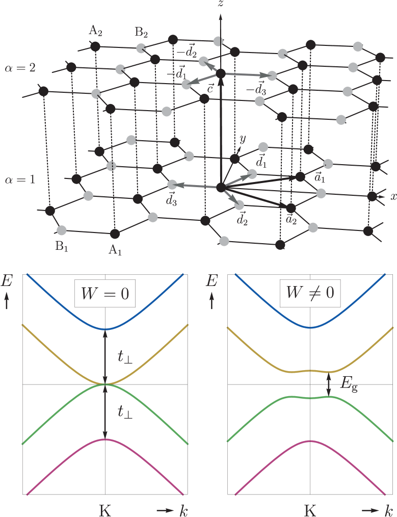
Figure 1: Graphene bilayer, with A carbon atoms in black and B carbon atoms in gray (top). Electronic spectrum near the K-point in absence (bottom left) and presence (bottom right) of a bias voltage $W$ between the layers.

Another means of influencing (mono- or bilayer) graphene’s electronic structure, currently receiving a lot of theoretical attention Gui2 ; Per ; Lee ; Mar ; Muc ; Muc2 ; Nan ; Raz ; Cho , is provided by mechanical deformations. It has e.g. been shown that it is possible to conceive inhomogeneous strains in single-layer graphene such that they act as a high uniform magnetic field, therefore resulting in strain-induced Landau levels and a zero-field quantum Hall effect Gui2 . In Ref. Per , Pereira et al. elaborated a tight-binding description for uniaxially strained single-layer graphene and predicted that a band gap can form upon deformations — along preferred directions — beyond 20%. Recent investigations on strained bilayer graphene include a standard tight-binding treatment of uniaxial strain Lee , a description of elastic deformations and electron-phonon coupling in bilayer graphene by means of pseudo-magnetic gauge fields Mar , the effect of strain on the Landau level spectrum and the quantum Hall effect Muc ; Muc2 and the effect of strain in combination with an external electric field Nan ; Raz .

In the present paper, we employ a nearest-neighbor tight-binding description and linear elasticity theory to show that a perpendicular strain component modifies the on-site energies of the two carbon sublattices in bilayer graphene, which can open a band gap at the K-point. The band gap is of a different nature than in the case of the “Mexican-hat-like” electronic dispersions. In addition, we consider the case of two graphene layers subjected to different (but uniform) strains, a scenario proposed recently and predicted — by means of ab initio calculations — to also lead to the opening of a band gap Cho . Uniform deformations parallel to the sheets are studied as well and are compared to the monolayer case Per .

II Strained bilayer-graphene

We first consider the unstrained AB (Bernal) stacking variant of bilayer graphene: two graphene layers (labeled 1 and 2) at $c=3.44$ Å apart with the A atoms of layer 2 sitting directly on top of the A atoms of layer 1 (Fig. 1, top). The B atoms of layer 1 and the B atoms of layer 2 have no direct neighbor in the opposite layer.

The band structure of bilayer graphene can be described within the tight-binding formalism. The nearest-neighbor tight-binding hamiltonian assumes one free $2p_{z}$ electron provided by each carbon atom and reads

$$H=V_{\text{A}}\sum_{\alpha}\sum_{\vec{X}_{\alpha}}c_{\vec{X}_{\alpha}}^{\dagger}c_{\vec{X}_{\alpha}}+V_{\text{B}}\left(\sum_{\vec{X}_{1}}c_{\vec{X}_{1}+\vec{d}_{1}}^{\dagger}c_{\vec{X}_{1}+\vec{d}_{1}}+\sum_{\vec{X}_{2}}c_{\vec{X}_{2}-\vec{d}_{1}}^{\dagger}c_{\vec{X}_{2}-\vec{d}_{1}}\right)\\ -t\Biggl{(}\sum_{\vec{X}_{1}}\sum_{l=1}^{3}\left[c_{\vec{X}_{1}}^{\dagger}c_{\vec{X}_{1}+\vec{d}_{l}}+c_{\vec{X}_{1}+\vec{d}_{l}}^{\dagger}c_{\vec{X}_{1}}\right]+\sum_{\vec{X}_{2}}\sum_{l=1}^{3}\left[c_{\vec{X}_{2}}^{\dagger}c_{\vec{X}_{2}-\vec{d}_{l}}+c_{\vec{X}_{2}-\vec{d}_{l}}^{\dagger}c_{\vec{X}_{2}}\right]\Biggr{)}\\ +t_{\perp}\sum_{\vec{X}_{1}}\left[c_{\vec{X}_{1}}^{\dagger}c_{\vec{X}_{1}+\vec{c}}+c_{\vec{X}_{1}+\vec{c}}^{\dagger}c_{\vec{X}_{1}}\right].$$ (1)

The index $\alpha$ stands for the layer (1 or 2), the vectors $\vec{X}_{\alpha}$ are the lattice sites of the A atoms of layer $\alpha$. Every A atom in layer 1 is surrounded by three B atoms at relative position vectors $\vec{d}_{1}=\frac{1}{2}a\vec{e}_{x}+\frac{\sqrt{3}}{2}a\vec{e}_{y}$, $\vec{d}_{2}=\frac{1}{2}a\vec{e}_{x}-\frac{\sqrt{3}}{2}a\vec{e}_{y}$ and $\vec{d}_{3}=-a\vec{e}_{x}$, where the bond length $a$ has a value of $1.42$ Å, and the A atoms in layer 2 have neighboring B atoms at relative positions $-\vec{d}_{l}$, $l=1,2,3$. The operators $c_{\vec{X}}^{\dagger}$ and $c_{\vec{X}}$ create and annihilate an electron at site $\vec{X}$, respectively. The vector $\vec{c}=c\vec{e}_{z}$ ($c=3.35$ Å) connects two nearest-neighbor atoms in different graphene sheets. Values for the intra- and inter-plane hopping energies $t$ and $t_{\perp}$ are obtained from fitting the tight-binding model to experimental data for graphite. Here we use the values quoted in Ref. Chu : $t=3.12$ eV and $t_{\perp}=0.377$ eV. The on-site energies $V_{\text{A}}$ and $V_{\text{B}}$ differ slightly due to the different environments of A and B atoms. The difference $\Delta=|V_{\text{A}}-V_{\text{B}}|\approx 0.009$ eV Chu is about two orders of magnitude smaller than the hopping parameter $t_{\perp}$ and is usually considered only in models going beyond the nearest-neighbor tight-binding hamiltonian (1) where also A${}_{\text{1}}$–B₂ and B₁–B₂ hoppings are taken into account (see e.g. Ref. Par1 ). We therefore put $V_{\text{A}}\approx V_{\text{B}}\equiv V$. The value of the on-site energies $V$ will turn out to be of critical importance when considering perpendicular strain; we will return to it later. For a comprehensive review on a complete tight-binding description of (unstrained) bilayer graphene, and in particular for a discussion of features in the electronic structure resulting from asymmetry of the diagonal (differences in on-site energies, $V_{\text{A}}\neq V_{\text{B}}$), we refer to Ref. Muc3 .

The direct-space hamiltonian (1) can be converted into a reciprocal-space hamiltonian by introducing four-component spinors

$$\Psi^{\dagger}(\vec{q}) =\left(\begin{array}[]{cccc}c_{\text{A}_{1}}^{\dagger}(\vec{q}),&c_{\text{B}_{1}}^{\dagger}(\vec{q}),&c_{\text{A}_{2}}^{\dagger}(\vec{q}),&c_{\text{B}_{2}}^{\dagger}(\vec{q})\end{array}\right),$$ (2b)

$$\Psi(\vec{q}) =\left(\begin{array}[]{c}c_{\text{A}_{1}}(\vec{q})\\ c_{\text{B}_{1}}(\vec{q})\\ c_{\text{A}_{2}}(\vec{q})\\ c_{\text{B}_{2}}(\vec{q})\end{array}\right),$$ (2g)

$$H =\sum_{\vec{q}}\Psi^{\dagger}(\vec{q}){\mathfrak{H}}(\vec{q})\Psi(\vec{q}).$$ (2h)

Here, the operators $c_{i}(\vec{q})$ ($i=\text{A}_{1},\text{B}_{1},\text{A}_{2},\text{B}_{2}$) are the discrete (lattice) Fourier transforms of $c_{\vec{X}_{i}}$:

$$c_{i}(\vec{q})=\frac{1}{\sqrt{N}}\sum_{\vec{X}_{i}}c_{\vec{X}_{i}}e^{-i\vec{q}\cdot\vec{X}_{i}},$$ (3)

where the $\vec{q}$-vectors of the first Brillouin zone are defined so that the properties $\sum_{\vec{q}}e^{i\vec{q}\cdot\vec{X}_{i}}=N\delta_{\vec{X}_{i},\vec{0}}$ and $\sum_{\vec{X}_{i}}e^{i\vec{q}\cdot\vec{X}_{i}}=N\delta_{\vec{q},\vec{0}}$ hold. The hamiltonian matrix $\mathfrak{H}(\vec{q})$ reads

$${\mathfrak{H}}(\vec{q}) =\left(\begin{array}[]{cccc}V&\zeta(\vec{q})&t_{\perp}&0\\ \zeta(\vec{q})^{*}&V&0&0\\ t_{\perp}&0&V&\zeta(\vec{q})^{*}\\ 0&0&\zeta(\vec{q})&V\\ \end{array}\right),$$ (8)

with

$$\zeta(\vec{q})=-t\sum_{l=1}^{3}e^{i\vec{q}\cdot\vec{d}_{l}}.$$ (9)

The band structure $\{E(\vec{q})\}$ is obtained by solving the secular equation $\det\bigl{(}\mathfrak{H}(\vec{q})-E(\vec{q})I_{4}\bigr{)}=0$, with $I_{4}$ the $4\times 4$ unit matrix, in the first Brillouin zone. At the K and K${}^{{}^{\prime}}$ points, two electron energy bands touch each other at the Fermi level, making the material a semi-metal (zero band gap).

Since the electronic properties of (bilayer) graphene are determined by the band structure near the K${}^{(^{\prime})}$ point — $\vec{q}_{\text{K}}=\frac{2\pi}{3a}\vec{e}_{x}+\frac{2\pi}{3\sqrt{3}a}\vec{e}_{y}$ and $\vec{q}_{\text{K}^{{}^{\prime}}}=\frac{2\pi}{3a}\vec{e}_{x}-\frac{2\pi}{3\sqrt{3}a}\vec{e}_{y}$ —, it is convenient to make a Taylor expansion of $\mathfrak{H}(\vec{q})$ around $\vec{q}_{\text{K}^{(^{\prime})}}$. With $\vec{q}=\vec{q}_{\text{K}}+\vec{k}$ and retaining only lowest-order terms in $k$, the hamiltonian matrix near $\vec{q}_{\text{K}}$ becomes

$${\mathfrak{H}}^{\text{K}}(\vec{k}) =\left(\begin{array}[]{cccc}V&\frac{3at}{2}ke^{i\phi}e^{-i\frac{\pi}{6}}&t_{\perp}&0\\ \frac{3at}{2}ke^{-i\phi}e^{i\frac{\pi}{6}}&V&0&0\\ t_{\perp}&0&V&\frac{3at}{2}ke^{-i\phi}e^{i\frac{\pi}{6}}\\ 0&0&\frac{3at}{2}ke^{i\phi}e^{-i\frac{\pi}{6}}&V\\ \end{array}\right).$$ (14)

Here, $\phi$ is defined via $k_{x}+ik_{y}=ke^{i\phi}$. For $\vec{q}=\vec{q}_{\text{K}^{{}^{\prime}}}+\vec{k}$, the hamiltonian matrix ${\mathfrak{H}}^{\text{K}^{{}^{\prime}}}(\vec{k})$ is the complex conjugate of ${\mathfrak{H}}^{\text{K}}(\vec{k})$. Note that the quantity $\frac{3at}{2}$ can be rewritten as $\hbar v_{\text{F}}$, with $v_{\text{F}}$ the Fermi velocity. Diagonalisation of (14) results in the dispersion shown in the left bottom of Fig. 1.

As mentioned in the introduction, the application of a bias voltage $W$ between layers 1 and 2 (replacing the elements ${\mathfrak{H}}^{\text{K}^{(^{\prime})}}_{11}(\vec{k})$ and ${\mathfrak{H}}^{\text{K}^{(^{\prime})}}_{33}(\vec{k})$ by $eW/2$ and ${\mathfrak{H}}^{\text{K}^{(^{\prime})}}_{22}(\vec{k})$ and ${\mathfrak{H}}^{\text{K}^{(^{\prime})}}_{44}(\vec{k})$ by $-eW/2$) results in a finite band gap McC2 ; Gui ; Oht ; McC3 ; Cas . However, this band gap lies not at $\vec{q}=\vec{q}_{\text{K}^{(^{\prime})}}$ but at a $q$-vector slightly away from $q_{\text{K}^{(^{\prime})}}$ (Fig. 1, bottom right), and its theoretical maximum value is $\lim_{W\longrightarrow\infty}E_{\text{g}}=t_{\perp}$. In the following, we will show that applying a strain to the bilayer graphene lattice can also lead to a band gap, which is not bounded by $t_{\perp}$.

In the presence of a displacement field $\vec{u}(\vec{X})$, the position of an atom formerly at $\vec{X}$ is $\vec{X}+\vec{u}(\vec{X})$. The effect of a small deformation of the lattice can be written as a correction $\delta H$ to the original hamiltonian $H$, with

$$\delta H=\delta V_{\text{A}}\sum_{\alpha}\sum_{\vec{X}_{\alpha}}c_{\vec{X}_{\alpha}}^{\dagger}c_{\vec{X}_{\alpha}}+\delta V_{\text{B}}\left(\sum_{\vec{X}_{1}}c_{\vec{X}_{1}+\vec{d}_{1}}^{\dagger}c_{\vec{X}_{1}+\vec{d}_{1}}+\sum_{\vec{X}_{2}}c_{\vec{X}_{2}-\vec{d}_{1}}^{\dagger}c_{\vec{X}_{2}-\vec{d}_{1}}\right)\\ -\sum_{\vec{X}_{1}}\sum_{l=1}^{3}\delta t_{l}\left[c_{\vec{X}_{1}}^{\dagger}c_{\vec{X}_{1}+\vec{d}_{l}}+c_{\vec{X}_{1}+\vec{d}_{l}}^{\dagger}c_{\vec{X}_{1}}\right]-\sum_{\vec{X}_{2}}\sum_{l=1}^{3}\delta t_{l}\left[c_{\vec{X}_{2}}^{\dagger}c_{\vec{X}_{2}-\vec{d}_{l}}+c_{\vec{X}_{2}-\vec{d}_{l}}^{\dagger}c_{\vec{X}_{2}}\right]\\ +\sum_{\vec{X}_{1}}\delta t_{\perp}\left[c_{\vec{X}_{1}}^{\dagger}c_{\vec{X}_{1}+\vec{d}}+c_{\vec{X}_{1}+\vec{d}}^{\dagger}c_{\vec{X}_{1}}\right].$$ (15)

Within the nearest-neighbor tight-binding approximation, the changes in on-site and hopping energy parameters $V_{\text{A}}$, $V_{\text{B}}$, $t$ and $t_{\perp}$ are related to changes in nearest-neighbor interatomic distances (bond lengths). We stress that it is therefore important to distinguish between A and B sites since they have different environments in the bilayer. As pointed out before, an A site has three in-plane nearest-neighbor B sites and one neighboring A site in the opposite layer at a distance $c+\delta c$; a B site has only the three surrounding in-plane A sites as nearest neighbors (see Fig. 1, top). Denoting the three (not necessarily equal) changed bond lengths between neighboring in-plane A and B atoms by $a_{l}=a+\delta a_{l}$ ($l=1,2,3$), we have for the corrections to the on-site energies to linear order in the deformations

$$\delta V_{\text{A}} =\sum_{l=1}^{3}\left.\frac{\partial V}{\partial a}\right|_{a}\delta a_{l}+\left.\frac{\partial V}{\partial c}\right|_{c}\delta c,$$ (16a)

$$\delta V_{\text{B}} =\sum_{l=1}^{3}\left.\frac{\partial V}{\partial a}\right|_{a}\delta a_{l}$$ (16b)

for each of the two layers. For the hopping parameters we have

$$\delta t_{l} =\left.\frac{\partial t}{\partial a}\right|_{a}\delta a_{l},$$ (17a)

$$\delta t_{\perp} =\left.\frac{\partial t_{\perp}}{\partial c}\right|_{c}\delta c.$$ (17b)

In the following we will drop the attributes $|_{a}$ and $|_{c}$. The link between the corrections $\delta V_{\text{A}}$, $\delta V_{\text{B}}$, $\delta t_{l}$ and $\delta t_{\perp}$ and the displacement field $\vec{u}(\vec{X})$ then comes from considering the bond length corrections $\delta a$ and $\delta c$. Details of the calculations and approximations involved are given in Appendix A; the resulting correction $\delta{\mathfrak{H}}(\vec{q})$ to the hamiltonian matrix ${\mathfrak{H}}(\vec{q})$ reads

$$\delta{\mathfrak{H}}(\vec{q})=\left(\begin{array}[]{cccc}\frac{3a}{2}\frac{\partial V}{\partial a}(\varepsilon_{xx}+\varepsilon_{yy})+c\frac{\partial V}{\partial c}\varepsilon_{zz}&\delta\zeta(\vec{q})&c\frac{\partial t_{\perp}}{\partial c}\varepsilon_{zz}&0\\ \delta\zeta(\vec{q})^{*}&\frac{3a}{2}\frac{\partial V}{\partial a}(\varepsilon_{xx}+\varepsilon_{yy})&0&0\\ c\frac{\partial t_{\perp}}{\partial c}\varepsilon_{zz}&0&\frac{3a}{2}\frac{\partial V}{\partial a}(\varepsilon_{xx}+\varepsilon_{yy})+c\frac{\partial V}{\partial c}\varepsilon_{zz}&\delta\zeta(\vec{q})^{*}\\ 0&0&\delta\zeta(\vec{q})&\frac{3a}{2}\frac{\partial V}{\partial a}(\varepsilon_{xx}+\varepsilon_{yy})\\ \end{array}\right),$$ (18)

with

$$\delta\zeta(\vec{q}) =-\sum_{l=1}^{3}\delta t_{l}e^{i\vec{q}\cdot\vec{d}_{l}}$$

$$=-a\frac{\partial t}{\partial a}e^{i\frac{1}{2}aq_{x}}e^{i\frac{\pi}{6}}\Big{(}\bigl{[}\frac{1}{2}\cos(\frac{\sqrt{3}}{2}aq_{y})+e^{-i\frac{3}{2}aq_{x}}\bigr{]}\varepsilon_{xx}+\frac{3}{2}\cos(\frac{\sqrt{3}}{2}aq_{y})\varepsilon_{yy}+\sqrt{3}i\sin(\frac{\sqrt{3}}{2}aq_{y})\varepsilon_{xy}\Bigr{)}.$$ (19)

Here, the quantities $\varepsilon_{ij}$ ($i,j=x,y,z$) are elements of the strain tensor $[\varepsilon]$, the general definition of which involve derivatives of the displacement field components to the coordinates. For the uniform displacements we mostly consider in this work the elements $\varepsilon_{ij}$ can be related to relative increments/decrements of the bond lengths occuring in the lattice (see Appendix A): $\vec{u}(\vec{X})=[\varepsilon]\vec{X}$.

The leading correction $\delta{\mathfrak{H}}^{\text{K}}$ to the hamiltonian matrix ${\mathfrak{H}}^{\text{K}}(\vec{k})$ at the K-point is $k$-independent and reads

$$\delta{\mathfrak{H}}^{\text{K}}=\left(\begin{array}[]{cccc}\frac{3a}{2}\frac{\partial V}{\partial a}(\varepsilon_{xx}+\varepsilon_{yy})+c\frac{\partial V}{\partial c}\varepsilon_{zz}&-i\frac{3a}{4}\frac{\partial t}{\partial a}(-\varepsilon_{xx}+\varepsilon_{yy}+2i\varepsilon_{xy})&c\frac{\partial t_{\perp}}{\partial c}\varepsilon_{zz}&0\\ i\frac{3a}{4}\frac{\partial t}{\partial a}(-\varepsilon_{xx}+\varepsilon_{yy}-2i\varepsilon_{xy})&\frac{3a}{2}\frac{\partial V}{\partial a}(\varepsilon_{xx}+\varepsilon_{yy})&0&0\\ c\frac{\partial t_{\perp}}{\partial c}\varepsilon_{zz}&0&\frac{3a}{2}\frac{\partial V}{\partial a}(\varepsilon_{xx}+\varepsilon_{yy})+c\frac{\partial V}{\partial c}\varepsilon_{zz}&i\frac{3a}{4}\frac{\partial t}{\partial a}(-\varepsilon_{xx}+\varepsilon_{yy}-2i\varepsilon_{xy})\\ 0&0&-i\frac{3a}{4}\frac{\partial t}{\partial a}(-\varepsilon_{xx}+\varepsilon_{yy}+2i\varepsilon_{xy})&\frac{3a}{2}\frac{\partial V}{\partial a}(\varepsilon_{xx}+\varepsilon_{yy})\\ \end{array}\right).\\$$ (20)

For $\vec{q}=\vec{q}_{\text{K}^{{}^{\prime}}}+\vec{k}$, the hamiltonian matrix correction $\delta{\mathfrak{H}}^{\text{K}^{{}^{\prime}}}$ is the complex conjugate of $\delta{\mathfrak{H}}^{\text{K}}$. The K-point hamiltonian correction for a strained single graphene layer, of the form

$$\left(\begin{array}[]{cc}g_{1}(\varepsilon_{xx}+\varepsilon_{yy})&g_{2}(\varepsilon_{xx}-\varepsilon_{yy}+2i\varepsilon_{xy})\\ g_{2}^{*}(\varepsilon_{xx}-\varepsilon_{yy}-2i\varepsilon_{xy})&g_{1}(\varepsilon_{xx}+\varepsilon_{yy})\end{array}\right),$$ (23)

has been derived before in the context of electron-phonon coupling in carbon nanotubes Suz , where the term proportional to $g_{1}$ is a deformation potential, a concept going back to Bardeen and Shockley Bar and the term proportional to $g_{2}$ corresponds to a bond-length change. However, to our knowledge, the derivation of the strained bilayer hamiltonian [Eqs. (18) – (19)] as given in Appendix A — with particular emphasis on the asymmetry on the diagonal — has not been reported before.

III Perpendicular uniform strain

We first consider the bilayer-specific possibility of perpendicular strain, $\varepsilon_{zz}$, associated with a change from the inter-layer distance $c$ to $c^{\prime}=c(1+\varepsilon_{zz})$. Putting the in-plane strain tensor elements to zero, the hamiltonian ${\mathfrak{H}}^{\text{K}}(\vec{k})+\delta{\mathfrak{H}}^{\text{K}}$ takes on the form

$${\mathfrak{H}}^{\text{K}}(\vec{k})+\delta{\mathfrak{H}}^{\text{K}}=\left(\begin{array}[]{cccc}V+c\frac{\partial V}{\partial c}\varepsilon_{zz}&\hbar v_{\text{F}}ke^{i\phi}&t_{\perp}+c\frac{\partial t_{\perp}}{\partial c}\varepsilon_{zz}&0\\ \hbar v_{\text{F}}ke^{-i\phi}&V&0&0\\ t_{\perp}+c\frac{\partial t_{\perp}}{\partial c}\varepsilon_{zz}&0&V+c\frac{\partial V}{\partial c}\varepsilon_{zz}&\hbar v_{\text{F}}ke^{-i\phi}\\ 0&0&\hbar v_{\text{F}}ke^{i\phi}&V\\ \end{array}\right).$$ (28)

The phase factors $e^{\mp i\frac{\pi}{6}}$ present in Eq. (14) have been eliminated by means of a redefinition of the operators for B sites [Eqs. (88a) – (88b)].

The symmetry-breaking along the diagonal exhibited by the hamiltionian matrix (28) is unusual since it distinguishes not between layers (as e.g. a bias voltage between the two layers would do) but between A and B sublattices. Interestingly, the hamiltonian (28) displays the possibility of the opening of a band gap at $k=0$: if

$$\left|c\frac{\partial V}{\partial c}\varepsilon_{zz}\right|>t_{\perp}+c\frac{\partial t_{\perp}}{\partial c}\varepsilon_{zz},$$ (29)

the degeneracy of the bands at $k=0$ is lifted, as illustrated in Fig. 2. (Criterion (29), an analytical result, holds when $t_{\perp}+c\frac{\partial t_{\perp}}{\partial c}\varepsilon_{zz}>0$, i.e. when $c\left|\frac{\partial t_{\perp}}{\partial c}\varepsilon_{zz}\right|$ is small compared to $t_{\perp}$.) Recently, Mucha-Kruczyński et al. Muc3 examined the asymmetry of the (unstrained) graphene bilayer hamiltonian’s diagonal. The possibility of band gap openings and electron-hole asymmetry, as encountered here in Fig. 2, due to different on-site energies, was realized. Here, we show that strain enhances the diagonal’s asymmetry [Eq. (18)] and that elastic deformations therefore provide a physical mechanism for the band structure modifications discussed in Ref. Muc3 .

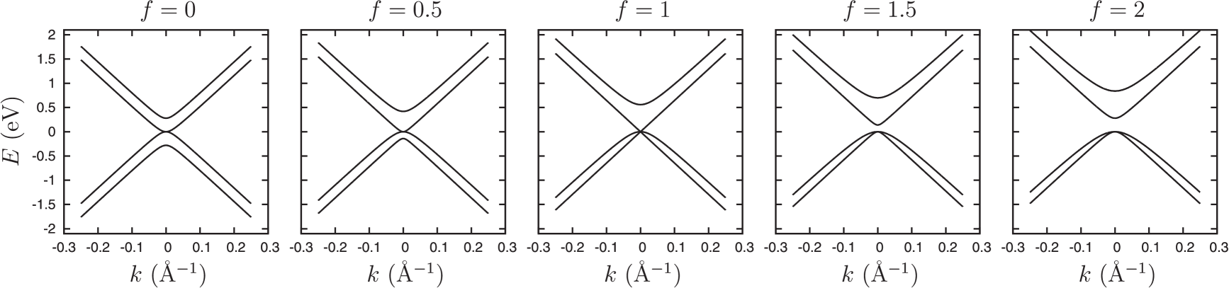
Figure 2: Low-$k$ band structure $E(k)$ for perpendicularly uniformly strained bilayer graphene for various values of $\left|c\frac{\partial V}{\partial c}\varepsilon_{zz}\right|=f\left(t_{\perp}+c\frac{\partial t_{\perp}}{\partial c}\varepsilon_{zz}\right)$.

To check whether the possibility of a strain-induced band gap is experimentally relevant, a more quantitative investigation of criterion (29) is in order. First, the variation of the hopping parameter $t_{\perp}$ with interlayer distance $c$ can be estimated using Harrison’s relation

$$\frac{\partial t_{\perp}}{\partial c}\approx-2\frac{t_{\perp}}{c},$$ (30)

which follows from an assumed inverse-square dependence of $t_{\perp}$ on $c$ Har . The inequality (29) then becomes

$$c\left|\frac{\partial V}{\partial c}\right|\left|\varepsilon_{zz}\right|\gtrsim t_{\perp}(1-2\varepsilon_{zz}).$$ (31)

For expansion ($\varepsilon_{zz}>0$), this can be rewritten as

$$c\left|\frac{\partial V}{\partial c}\right|\gtrsim t_{\perp}\left(\frac{1}{\varepsilon_{zz}}-2\right),$$ (32)

while for contraction ($\varepsilon_{zz}<0$), one obtains

$$c\left|\frac{\partial V}{\partial c}\right|\gtrsim t_{\perp}\left(-\frac{1}{\varepsilon_{zz}}+2\right).$$ (33)

The intra- and inter-plane hopping parameters have values of $t=3.12$ eV and $t_{\perp}=0.377$ eV, respectively. The interplane distance is $c=3.35$ Å, so that $\frac{t_{\perp}}{c}=0.113$ eV/Å. Using these values, we have plotted the quantities $\frac{t_{\perp}}{c}\left(\frac{1}{\varepsilon_{zz}}-2\right)$ and $\frac{t_{\perp}}{c}\left(\frac{1}{|\varepsilon_{zz}|}+2\right)$ in Fig. 3. Interestingly, it follows that the band gap formation criterion is reached more easily (smaller $|\varepsilon_{zz}|$) in the case of expansion.

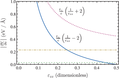
Figure 3: (Color online) Plots of the variation of $\frac{t_{\perp}}{c}\left(\frac{1}{\varepsilon_{zz}}-2\right)$ (blue, full line, expansion) and $\frac{t_{\perp}}{c}\left(\frac{1}{\varepsilon_{zz}}+2\right)$ (violet, dashed line, contraction) with $\varepsilon_{zz}$. The two horizontal lines represent the values of $\left|\frac{\partial V}{\partial c}\right|$ resulting from using the two extreme values for $V$ considered in the present work — $V=-2$ eV (olive, dashed-dotted line) and $V=-0.25$ eV (green, dashed line).

To obtain a physically meaningful estimate for the quantity $\left|\frac{\partial V}{\partial c}\right|$ we proceed as follows. First, we recall the tight-binding definition of $V$:

$$V\equiv\varepsilon_{2p_{z}}=\int d\vec{r}\psi^{*}(\vec{r})U(\vec{r})\psi(\vec{r}).$$ (34)

Here, $\psi(\vec{r})$ is the $2p_{z}$ electron wave function for a carbon atom, and $U(\vec{r})$ is the periodic potential of the lattice. Suprisingly, while the tight-binding formalism is a standard method for modelling band structures — especially for carbon structures —, a numerical value for $V\equiv\varepsilon_{2p_{z}}$ has not yet been established in the literature. The plausible reason is that when the difference between $V_{\text{A}}$ and $V_{\text{B}}$ is neglected (see Sect. II), the presence of $V$ on the diagonal of the hamiltonian matrix merely results in an overall shift of the energy bands, making its actual value redundant. In Ref. Rei , Reich et al. present a detailed comparison of tight-binding and ab initio energy dispersion calculations for graphene and provide fits of the tight-binding parameters to the band structures obtained by density-functional theory. Two variants were considered: one fitting the full $M\Gamma KM$-path in $k$-space and one where only $\vec{k}$-vectors yielding optical transitions with energies less than 4 eV were taken into account, resulting in $\varepsilon_{2p_{z}}=-0.28$ eV and $-2.03$ eV, respectively. We will therefore consider the range $-0.25$ eV $\geq\varepsilon_{2p_{z}}\geq-2$ eV. The simplest way of modelling $U(\vec{r})$ is to put positively charged ions (charge $1e>0$) at $\vec{r}=\vec{0}$ and $\vec{r}=c^{\prime}\vec{e}_{z}$:

$$U(\vec{r})\propto-\frac{1}{|\vec{r}|}-\frac{1}{|\vec{r}-c^{\prime}\vec{e}_{z}|}=-\frac{1}{r}-\frac{1}{\sqrt{r^{2}-2c^{\prime}r\cos\theta+c^{\prime 2}}},$$ (35)

where spherical coordinates have been introduced. For the carbon $2p_{z}$ electron wave function, we follow the common practice of taking the hydrogen-like $2p_{z}$ orbital:

$$\psi(\vec{r})\propto re^{-\frac{r}{2a_{0}}}\cos\theta,$$ (36)

where $a_{0}=0.529$ Å is the Bohr radius. We then get for $V$ the expression

$$V=C\int_{0}^{\infty}r^{2}dr\int_{0}^{\pi}\sin\theta d\theta r^{2}e^{-\frac{r}{a_{0}}}\cos^{2}\theta\left(-\frac{1}{r}-\frac{1}{\sqrt{r^{2}-2c^{\prime}r\cos\theta+c^{\prime 2}}}\right),$$ (37)

where the proportionality factors left unspecified in Eqs. (35) and (36), together with the factor $2\pi$ coming from the azimuthal integration, have been collected into the factor $C$. The integrals

$$S_{nc^{\prime}}(r)=\int_{0}^{\pi}d\theta\frac{\sin\theta\cos^{2}\theta}{\sqrt{r^{2}-2nc^{\prime}r\cos\theta+(nc^{\prime})^{2}}}$$ (38)

entering Eq. (37) can be solved analytically:

$$S_{0}(r) =\frac{2}{3r},$$ (39a)

$$S_{nc^{\prime}>0}(r) =\left\{\begin{array}[]{l}\frac{2}{15}\frac{5(nc^{\prime})^{2}+2r^{2}}{(nc^{\prime})^{3}}\text{ if $0\leq r\leq nc^{\prime}$}\\ \frac{2}{15}\frac{2(nc^{\prime})^{2}+5r^{2}}{r^{3}}\text{ if $r>nc^{\prime}$}\end{array}\right..$$ (39d)

For $c^{\prime}=c=3.35$ Å, the integral

$$D(c)=\int_{0}^{\infty}drr^{4}e^{-\frac{r}{a_{0}}}\bigl{(}S_{0}(r)+S_{1c}(r)\bigr{)}$$ (40)

has the value $D(c)=0.539$ Å⁴. From $V=CD(c)$ we can then obtain the “calibration value” $C=V/D(c)$. For the values $V=-0.25$ eV and $V=-2$ eV, we obtain $C=-0.463$ eV/Å^-4 and $C=-3.709$ eV/Å^-4, respectively. The dependence of $V$ on $c^{\prime}$ reads $V(c^{\prime})=CD(c^{\prime})$, it is visualised in Fig. 4. Clearly, a linear approximation in the range $-0.25\leq\varepsilon_{zz}\leq 0.25$ is justifiable, and the value of $\frac{\partial V}{\partial c}$ can be easily determined numerically. We find $\frac{\partial V}{\partial c}=0.0287$ eV/Å and $0.230$ eV/Å for $V=-0.25$ eV and $V=-2$ eV, respectively; these values are marked by horizontal lines in Fig. 3.

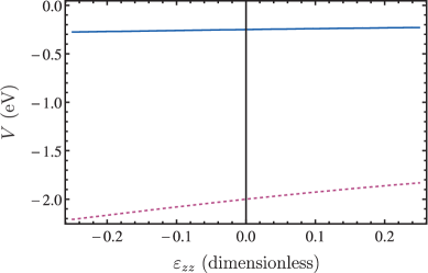
Figure 4: Plots of the variation of $V(c^{\prime})$ with $c^{\prime}=c(1+\varepsilon_{zz})$ for $V(c)=-0.25$ eV (blue, full line) and $V(c)=-2$ eV (violet, dashed line).

Within the present model, it follows that in the case of a large tight-binding on-site energy parameter ($|V|=2$ eV), a band gap opens for positive strains larger than $\varepsilon_{zz}\approx 0.25$ (see Fig. 3), corresponding to interlayer distances larger than $c^{\prime}\approx 4.19$ Å. For $\varepsilon_{zz}\approx 30\%$, the band gap’s magnitude is about $125$ meV (Fig. 2, $f=1.5$).

We recall that formally, criterion (29) is valid when the right-hand side is positive, i.e. when $\varepsilon_{zz}<0.5$, hence the upper limit of $\varepsilon_{zz}=0.5$ in Fig. 3. Going beyond strains of $50\%$ (both positive and negative) would be well outside the validity of the assumption of small displacements $\vec{u}(\vec{X})$, on which the hamiltonian matrix (18) relies (see Appendix A). For $\varepsilon\sim 0.25$, neglected contributions are of the order $\varepsilon^{2}\sim 0.063$ which is still acceptable. Similarly, we point out that the unphysical behavior of an ever increasing band gap with increasing $\varepsilon_{zz}$ must become invalid when linear elasticity, i.e. the assumption of small bond length changes [Eq. (52)], fails.

Based on the foregoing elaborations, stating that the opening of a strain-induced band gap by pulling apart the two graphene layers may be experimentally observed is a fair conclusion. Our main purpose here is not to provide accurate predictions but rather to point out the consequences of the symmetry-breaking along the diagonal in the hamiltonian of strained bilayer graphene. Accurate density-functional theory calculations could provide better numerical estimates, but most importantly, experiments should be undertaken to investigate the effect on the band structure upon pushing together or pulling apart the graphene layers.

IV Symmetric uniform $xy$-strain

We next consider pulling or pushing the bilayer in a direction parallel to the graphene sheets ($\varepsilon_{zz}=0$). The tight-binding hamiltonian then reads

$${\mathfrak{H}}(\vec{k})=\left(\begin{array}[]{cccc}V+\frac{3a}{2}\frac{\partial V}{\partial a}(\varepsilon_{xx}+\varepsilon_{yy})&\zeta(\vec{q})+\delta\zeta(\vec{q})&t_{\perp}&0\\ \zeta^{*}(\vec{q})+\delta\zeta^{*}(\vec{q})&V+\frac{3a}{2}\frac{\partial V}{\partial a}(\varepsilon_{xx}+\varepsilon_{yy})&0&0\\ t_{\perp}&0&V+\frac{3a}{2}\frac{\partial V}{\partial a}(\varepsilon_{xx}+\varepsilon_{yy})&\zeta^{*}(\vec{q})+\delta\zeta^{*}(\vec{q})\\ 0&0&\zeta(\vec{q})+\delta\zeta(\vec{q})&V+\frac{3a}{2}\frac{\partial V}{\partial a}(\varepsilon_{xx}+\varepsilon_{yy})\\ \end{array}\right).\\$$ (41)

The $4$ solutions of the corresponding secular equation are

$$E_{\pm,\pm}(\vec{q})=\pm\sqrt{\frac{t_{\perp}^{2}+2|\zeta(\vec{q})+\delta\zeta(\vec{q})|^{2}\pm t_{\perp}\sqrt{t_{\perp}^{2}+4|\zeta(\vec{q})+\delta\zeta(\vec{q})|^{2}}}{2}}.$$ (42)

There can only be a band gap when $\zeta(\vec{q})+\delta\zeta(\vec{q})$ differs from zero for all $\vec{q}$-vectors. The same condition arises from the monolayer strain problem, where the $2$ solutions of the secular equation read $E_{\pm}(\vec{q})=\pm|\zeta(\vec{q})+\delta\zeta(\vec{q})|$ (leading to the Dirac cone at the K${}^{\text{(${}^{\prime}$)}}$-point for $\delta\zeta(\vec{q})=0$). Pereira et al. Per have investigated the behavior of $|\zeta(\vec{q})+\delta\zeta(\vec{q})|$ in detail. Using the isotropy of a 2D hexagonal lattice, the strain tensor can be written as

$$[\varepsilon]=\left(\begin{array}[]{cc}\cos^{2}\theta-\sigma\sin^{2}\theta&(1+\sigma)\cos\theta\sin\theta\\ (1+\sigma)\cos\theta\sin\theta&\sin^{2}\theta-\sigma\cos^{2}\theta\end{array}\right),$$ (45)

with $\theta$ the angle between the tension $\vec{T}$ and the $y$-axis ($\vec{T}=T\cos(\pi/2+\theta)\vec{e}_{x}+T\sin(\pi/2+\theta)\vec{e}_{y}$) Perfootnote , and $\sigma$ the Poisson ratio, which takes the graphite value of $0.165$ which we choose in the remainder Bla . The conclusions made by Pereira et al. are that (i) the minimal strain required for opening a gap is about $23\%$, that (ii) tension along the zig-zag direction ($\theta=0,\pi/3,2\pi/3$) is optimal for the opening of a band gap, and that (iii) tension along the armchair direction ($\theta=\pi/2,5\pi/6,11\pi/6)$ never results in a band gap. From Eq. (42) it follows that the inter-plane coupling $t_{\perp}$ does not play any role and that the same conclusions are valid for the bilayer.

V Asymmetric uniform $xy$-strain

Finally, we consider the possibility of applying different strains (parallel to the bilayer) to the two layers $\alpha=1$ and $\alpha=2$. In Ref. Cho , ab initio calculations of a graphene bilayer’s band structure were performed for the situation where one of the two layers is subjected to positive strain along the zig-zag or armchair direction (without the elastic response in the perpendicular direction). Here, we consider a more general situation. We choose to let layer $1$ intact ($[\varepsilon]=[0]$), while layer $2$ is pushed or pulled ($[\varepsilon]\neq[0]$). Any pushing/pulling direction is allowed; the elastic response is taken into account by using expression (45) for the strain tensor of layer 2.

The deformation of layer $2$ introduces a mismatch between the two honeycomb lattices. For infinitesimally small deformations $\varepsilon$, the crystallographically correct unit cell of the bilayer — the “least common multiple” of the unit cells of the two layers — becomes infinitely large. For practically feasible descriptions of the asymetrically distorted bilayer one is forced to choose deformations that lead to not-too-large unit cells, resulting in a discrete set of strain values $\varepsilon$. For example, for their ab initio calculations, Choi et al. Cho considered minimal zig-zag strains of about $2\%$, requiring a supercell of $51$ unit cells in layer $1$ and $50$ in layer $2$. A tight-binding description faces the same mismatching problem. Apart from the necessity to set up a larger hamiltonian matrix, the inter-layer hopping parameters would have to be carefully reconsidered. Indeed, in the case of asymmetric strain, the A₂ atom originally directly above a particular A₁ atom now has a different position, while a B₁ atom may now have a direct (or almost direct) neighbor above. In a way, the structure becomes a mix of AB and AA stacking Cho . A similar issue was addressed recently in Ref. San : spatial modulations in the bilayer interlayer hopping arising due to elastic shearing or twisting were shown to lead to a non-Abelian gauge potential in the description of the low-energy electronic spectrum.

Designing the full tight-binding matrix with correctly interpolated inter-layer hopping parameters is a formidable task, the outcome of which would still only be a limited set of finite accessible strains $\varepsilon$. As a compromise, we therefore consider the following small-$\vec{k}$ hamiltonian:

$${\mathfrak{H}}(\vec{k})=\left(\begin{array}[]{cccc}V&\hbar v_{\text{F}}ke^{i\phi}&t_{\perp}&0\\ \hbar v_{\text{F}}ke^{-i\phi}&V&0&0\\ t_{\perp}&0&V+\frac{3a}{2}\frac{\partial V}{\partial a}(\varepsilon_{xx}+\varepsilon_{yy})&\hbar v_{\text{F}}ke^{-i\phi}+i\frac{3a}{4}\frac{\partial t}{\partial a}(-\varepsilon_{xx}+\varepsilon_{yy}-2i\varepsilon_{xy})\\ 0&0&\hbar v_{\text{F}}ke^{i\phi}-i\frac{3a}{4}\frac{\partial t}{\partial a}(-\varepsilon_{xx}+\varepsilon_{yy}+2i\varepsilon_{xy})&V+\frac{3a}{2}\frac{\partial V}{\partial a}(\varepsilon_{xx}+\varepsilon_{yy})\\ \end{array}\right),\\$$ (46)

where the parameter $t_{\perp}$ has to be interpreted as representing the average hopping between the two layers. The application of asymmetric plain affects both the diagonal and the off-diagonal elements; the resulting band structure is therefore non-trivial and worth investigating. Diagonalising the hamiltonian (LABEL:hamIIIa) results in the following secular equation:

$$\bigl{(}E(\vec{k})^{2}-|\zeta(\vec{k})|^{2}\bigr{)}\Bigl{[}\bigl{(}F-E(\vec{k})\bigr{)}^{2}-|\zeta(\vec{k})+\delta\zeta|^{2}\Bigr{]}+t_{\perp}^{2}E(\vec{k})\bigl{(}F-E(\vec{k})\bigr{)}=0,$$ (47)

with

$$F =\frac{3a}{2}\frac{\partial V}{\partial a}(\varepsilon_{xx}+\varepsilon_{yy})=\frac{3a}{2}\frac{\partial V}{\partial a}\varepsilon(1-\sigma),$$ (48a)

$$\zeta(\vec{k}) =\frac{3at}{2}ke^{i\phi},$$ (48b)

$$\delta\zeta =-i\frac{3a}{4}\frac{\partial t}{\partial a}(-\varepsilon_{xx}+\varepsilon_{yy}+2i\varepsilon_{xy})=\frac{3a}{4}\frac{\partial t}{\partial a}\varepsilon\bigl{[}i(1-\sigma)\cos(2\theta)+(1+\sigma)\sin(2\theta)\bigr{]}.$$ (48c)

Note that the argument $\phi=\tan^{-1}\frac{k_{y}}{k_{x}}$ does, in general, not cancel out, and that the full 2D dependence of $E(k_{x},k_{y})$ has to be considered. Note also that upon replacing $\varepsilon$ by $-\varepsilon$ in Eqs. (47) – (48c), the secular equation remains invariant if $E$ changes sign and the phase $\phi$ is shifted by $\pi$. Hence, the substitution $\varepsilon\longrightarrow-\varepsilon$ only leads to a band inversion and it suffices, as far as the opening of a band gap concerns, to consider $\varepsilon\geq 0$.

The change in band structure comes from the interplay between the values of $a\frac{\partial V}{\partial a}$, $a\frac{\partial t}{\partial a}$ and $t_{\perp}$. To obtain an estimate for $\frac{\partial t}{\partial a}$ we use the equivalent of relation (30):

$$\frac{\partial t}{\partial a}=-2\frac{t}{a}=-4.394\text{ eV/{\AA}}.$$ (49)

Note that Harrison’s relation [Eqs. (30) and (49)] should be taken as a rule of thumb rather than as an exact result Har . Other (experimental or theoretical) values than $2$ for $\eta=-\frac{\partial\ln t}{\partial\ln a}$ circulate in the literature (e.g. $\eta=3.6$ Pie , $\eta=3$ Bas or $\eta=1.1$ Her ). As it is our aim to make qualitative conclusions, we have used $\eta=2$.

For $\frac{\partial V}{\partial a}$, we proceed as for $\frac{\partial V}{\partial c}$ in Sect. III and put a charge at $\vec{r}=\vec{0}$ and $\vec{r}=a^{\prime}\vec{e}$, with $\vec{e}$ any unit vector perpendicular to the $z$-axis (a convenient choice is $\vec{e}=\vec{e}_{x}$) to mimic the periodic lattice potential :

$$U(\vec{r})\propto-\frac{1}{|\vec{r}|}-\frac{1}{|\vec{r}-a^{\prime}\vec{e}|}=-\frac{1}{r}-\frac{1}{\sqrt{r^{2}-2a^{\prime}r\sin\theta\cos\phi+a^{\prime 2}}}.$$ (50)

Using the definition (34) for $V(a^{\prime})$, we numerically calculate the derivative $\left.\frac{\partial V}{\partial a}\right|_{a^{\prime}=a}$ and obtain $0.0439$ eV/Å and $0.351$ eV/Å for the cases $V(a^{\prime}=a)=-0.25$ eV and $V(a^{\prime}=a)=-2$ eV, respectively. Inserting the value $\frac{\partial V}{\partial a}=0.351$ eV/Å, we observe the opening of a band gap for arbitrarily small values of $\varepsilon$. In Fig. 5, low-$\vec{k}$ band structures are shown for a few choices of $(\varepsilon,\theta)$. The $(k_{x},k_{y})$ electronic dispersions always consist of two facing doubly-peaked surfaces. This can result in an indirect band gap [Fig. 5(a)], but also in indirect band crossings [Figs. 5(b) and (c)]. An inspection of the ranges $0\leq\varepsilon\leq 0.25$ and $0\leq\theta\leq\pi$ allows to conclude that (i) above a critical value for the strain, only indirect band crossings are observed and (ii) the angle $\theta$ has little or no influence on the presence/absence of a band gap. The former conclusion agrees with the observation of Choi et al. Cho of a decrease of the band gap for zig-zag strains larger than $\varepsilon\approx 9\%$. As for the dependence of the band gap on $\theta$, Choi et al. Cho found that in the case of armchair strains, no band gap appears at all. We recall that we allow for an elastic restoring force perpendicular to the pulling/pushing direction which results in a dependence between $\varepsilon_{xx}$, $\varepsilon_{xy}$ and $\varepsilon_{yy}$ [Eq. (45)]. In our model, this isotropy makes the band gap development independent of $\theta$.

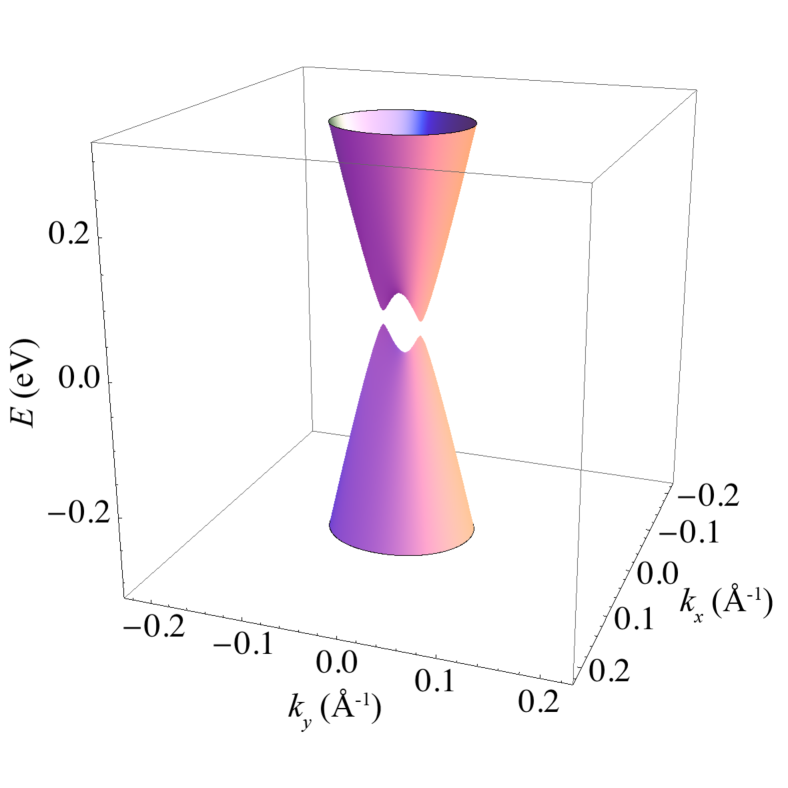
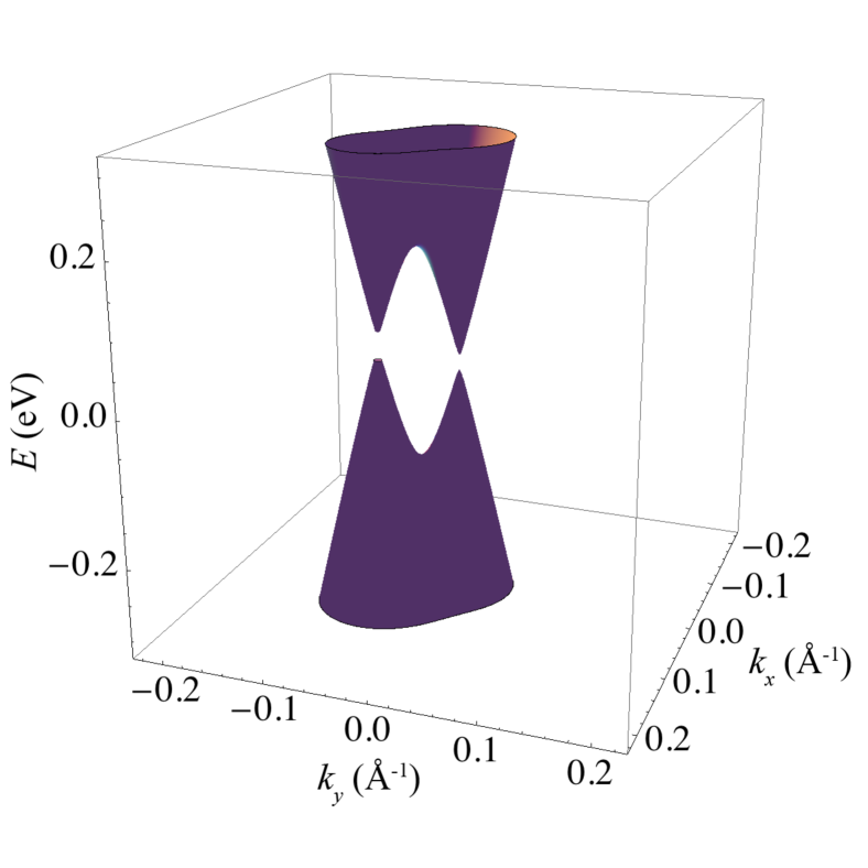
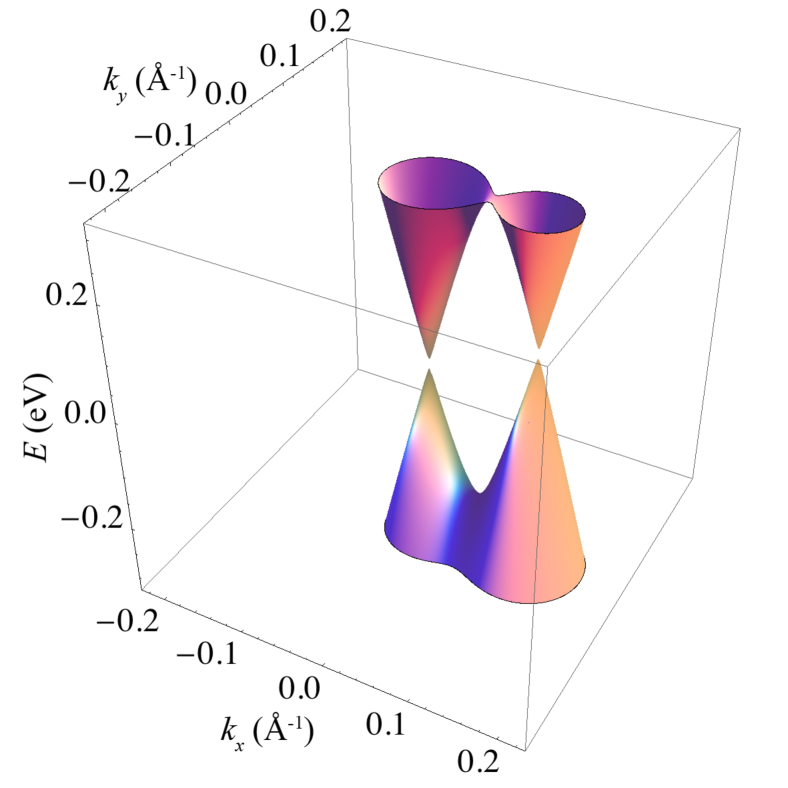
Figure 5: Band structure of asymmetrically in-plane deformed bilayer graphene near the K-point, for $\frac{\partial V}{\partial a}=0.351$ eV/Å: (a) $\varepsilon=0.05$, $\theta=0$, (b) $\varepsilon=0.1$, $\theta=\pi/8$, (c) $\varepsilon=0.15$, $\theta=\pi/4$.

A true (but indirect) band gap is only observed for small strains $\varepsilon$, as e.g. in Fig. 5(a) ($\varepsilon=0.05$, $\theta=0$, $\Delta E_{\text{g}}\approx 10$ meV). The maximal band gap turns out to depend on the magnitude of $\frac{\partial V}{\partial a}$, not unlike the situation in Sect. III for transversal strain where the value of $\frac{\partial V}{\partial c}$ is critical. For the value $\frac{\partial V}{\partial a}=0.0439$ eV/Å, corresponding to $V(a)=-0.25$ eV, the band gap for $\varepsilon=0.05$ and $\theta=0$ reduces to $\Delta E_{\text{g}}\approx 1$ meV). For the artificially large value of $\frac{\partial V}{\partial a}=1$ eV, we find (Fig. 6) $\Delta E_{\text{g}}=25$ meV. At this point we remark that one can identify $\frac{3a}{2}\frac{\partial V}{\partial a}$ with the deformation potential $g_{1}$ entering the strained monolayer hamiltonian (23), whose value for graphite is about $16$ eV Sug2 . For $\frac{\partial V}{\partial a}$ one therefore has approximately $7.5$ eV Å, which suggests that larger values of $\frac{\partial V}{\partial a}$ may indeed be more appropriate. Obviously, experiments and/or ab initio calculations should be carried out to clarify the parameters’ values.

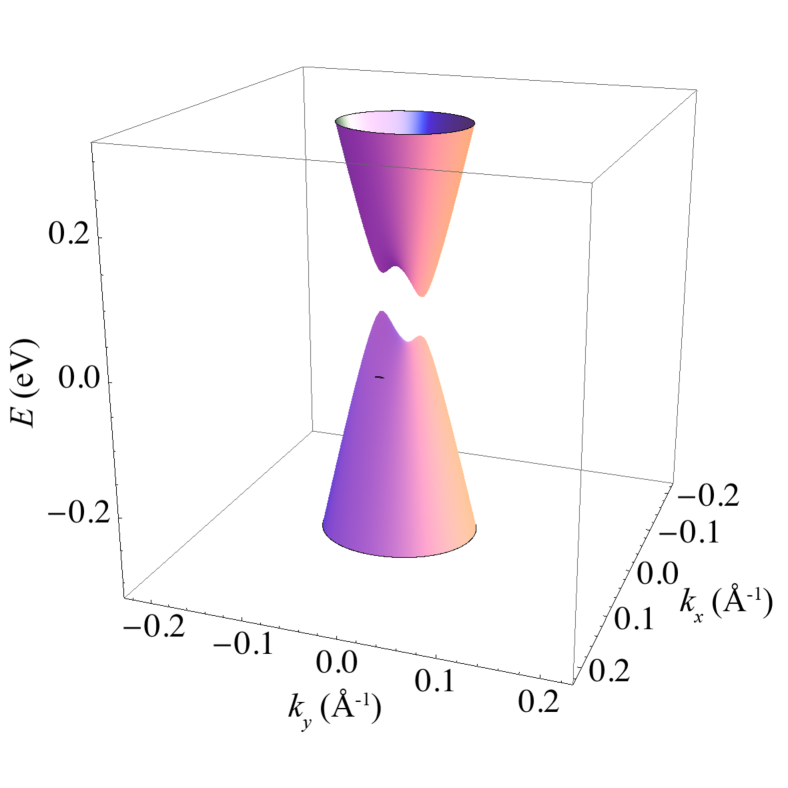
Figure 6: Band structure of asymetrically in-plane deformed bilayer graphene near the K-point, for $\frac{\partial V}{\partial a}=1$ eV/Å, $\varepsilon=0.05$ and $\theta=0$.

In conclusion, hamiltionian (LABEL:hamIIIa), a possible model for describing the effect of asymmetric lateral strains in bilayer graphene, results in indirect band gaps for small strains ($\varepsilon\approx 5\%$). For larger strains ($\varepsilon\gtrsim 10\%$), overlapping indirect bands result in a gapless spectrum. No critical directional strain dependence is observed, which comes from the anisotropy of the 2D hexagonal lattice.

VI conclusions

Applying strain to a graphene bilayer alters its electronic structure. Using the simplest tight-binding model, featuring only nearest-neighbor intra- and inter-plane hopping ($t$ and $t_{\perp}$), we have shown that for the AB (Bernal) stacking of two graphene sheets, several band gap scenarios are possible.

A first possibility is to push (pull) the bilayer’s two graphene sheets towards (away from) each other. As a consequence of the different neighborhoods experienced by A and B carbon atoms, the change in on-site tight-binding energies results in a symmetry breaking which, for large enough strains, opens a band gap. We find that pulling and pushing are inequivalent; the former is more effective in producing a gap. Predictions of the minimally required strain to open a band gap critically depend on values for the changes in on-site and inter-layer hopping energies with inter-plane distance ($\frac{\partial V}{\partial c}$ and $\frac{\partial t_{\perp}}{\partial c}$). These quantities are not readily available from the literature. We therefore rely on rules of thumb to make acceptable estimates, and find that for pulling, a band gap opens from $\varepsilon_{zz}=0.25$ onwards. For $\varepsilon_{zz}\approx 30\%$, the band gap is about $125$ meV. For pushing, the critical strain is well beyond $50\%$. Note that a strain of $50\%$ would require a pressure of $p=0.5c_{44}\approx 2$ GPa (taking for the elastic constant $c_{44}$ the value of graphite, $c_{44}=4.18$ GPa MicVerPRB2008 ), which is experimentally feasible. While bringing the two layers close together can be realized by applying high pressure, pulling the graphene sheets away from each other is an experimental challenge. A possible indirect way to do so would be to intercalate the bilayer; recently, for example, Li atoms have successfully been intercalated between two graphene sheets Sug . Interestingly, we find that at the critical strain, the electronic dispersion near the K-point consists of a triple degeneracy of two crossing linear bands (Dirac cone) and one parabolic band. This result shows that under certain symmetry-breaking strain conditions, bilayer graphene can exhibit Dirac fermions. Normally, Dirac fermions only occur in graphene multilayers consisting of an odd number of graphene sheets Par2 . The asymmetry of the hamiltonian matrix diagonal lies at the basis of the band structure modifications observed in Fig. 2. It was already recognized before Muc3 that intra-layer on-site energy differences can lead to band gaps of a different type than the “Mexican-hat-like” band gap band structures McC2 ; Gui ; Oht ; McC3 ; Cas associated with inter-layer energy differences e.g. induced by the application of a bias. In the present work, we have shown that uniform perpendicular strain provides a physical means for enhancing the intra-layer energy differences.

A second possibility is to push/pull parallel to the bilayer (symmetric uniform strain). It turns out that the criterion for opening a band gap is the same as for monolayer graphene; the inter-plane coupling $t_{\perp}$ does not play any role. The conclusions made by Pereira et al. Per for the monolayer can be transferred to the bilayer; a strain along the zig-zag direction larger than $\sim 23\%$ results in a band gap, while pushing/pulling along the armchair direction never leads to a gap.

Finally, we considered asymmetric uniform strain: the two graphene sheets experience different strains parallel to the bilayer. Assuming a tight-binding hamiltonian matrix where $t_{\perp}$ represents an average inter-plane hopping, we obtain the interesting result that a small finite strain, in any direction, immediately opens a band gap. The maximal band gap depends, similarly to the case of transversal strain, on the interplay of the quantities $\frac{\partial V}{\partial a}$ and $\frac{\partial t}{\partial a}$, reliable estimates for which are hard to derive. The observed band gaps are relatively small — $\Delta E_{\text{g}}\approx 10$ meV. The advantage, however, is that there is no strain barrier. Rather, beyond a certain strain (typically $10\%$), bands start to indirectly overlap and destroy the gap. As opposed to the case of uniform symmetric strain, no dependence on the strain direction was obtained — a consequence of the isotropy of a hexagonal lattice and of taking the elastic response in the perpendicular direction into account. Pushing and pulling are equivalent. We point out that the observed band gaps are indirect, which is relevant for possible opto-electronic applications. Our results are in qualitative agreement with recent ab initio calculations of the electronic structure of similarly asymmetrically strained bilayer graphene Cho .

Although having provided estimates for strains $\varepsilon$ required for the opening of a band gap and associated band gap magnitudes $\Delta E_{\text{g}}$, we wish to emphasize the qualitative aspect of our results. Irrespective of the precise values of the tight-binding parameters and derived quantities, it is the particular structure of the graphene bilayer that, when deformed, allows for gapped electronic structures. In our opinion, the various ways shown here in which a band gap can be induced in bilayer graphene by deformations should stimulate experimental investigations on the possibility of strain-engineering bilayer graphene’s electronic properties. Recalling graphene’s high strength, this should be feasible. In addition, we suggest that the theoretical models presented here be reconsidered by means of precise ab initio calculations.

Appendix A Strain

As described in the main text, deformations of the bilayer graphene carbon network enter the tight-binding formalism via bond length changes [Eqs. (16a) – (17b)]. In this Appendix, we elaborate the expressions for $\delta a_{l}$ and $\delta c$ and the strained graphene bilayer tight-binding hamiltonian.

A.1 Continuous description. Long-wavelength limit

In general, one has

$$a+\delta a_{l} =\Bigl{|}\vec{X}+\vec{d}_{l}+\vec{u}(\vec{X}+\vec{d}_{l})-\bigl{(}\vec{X}+\vec{u}(\vec{X})\bigr{)}\Bigr{|}$$

$$=\sqrt{a^{2}+2\vec{d}_{l}\cdot\bigl{(}\vec{u}(\vec{X}+\vec{d}_{l})-\vec{u}(\vec{X})\bigr{)}+\bigl{|}\vec{u}(\vec{X}+\vec{d}_{l})-\vec{u}(\vec{X})\bigr{|}^{2}}.$$ (51)

Assuming small bond length changes $\delta a_{l}$, we retain only first-order terms:

$$a+\delta a_{l}\approx a\left(1+\frac{1}{a^{2}}\vec{d}_{l}\cdot\bigl{(}\vec{u}(\vec{X}+\vec{d}_{l})-\vec{u}(\vec{X})\bigr{)}\right),$$ (52)

so that

$$\delta a_{l}\approx\frac{1}{a}\vec{d}_{l}\cdot\bigl{(}\vec{u}(\vec{X}+\vec{d}_{l})-\vec{u}(\vec{X})\bigr{)}.$$ (53)

In the case of small bond length changes, the differences between displacements at neighboring sites $\bigl{|}\vec{u}(\vec{X}+\vec{d}_{l})-\vec{u}(\vec{X})\bigr{|}$ must be small as well. In other words, the displacement field $\vec{u}$ is a slowly varying (vector) function of $\vec{X}$, implying that a linearisation of $\vec{u}$ at $\vec{X}$ approximates $\vec{u}$ at $\vec{X}+\vec{d}_{l}$ well enough. In this so-called long-wavelength limit we then have

$$\vec{d}_{l}\cdot\bigl{(}\vec{u}(\vec{X}+\vec{d}_{l})-\vec{u}(\vec{X})\bigr{)} \approx\left.(\vec{d}_{l}\cdot\vec{\nabla})(\vec{d}_{l}\cdot\vec{u})\right|_{\vec{X}}.$$ (54)

The operator $\vec{\nabla}=\left(\frac{\partial}{\partial x},\frac{\partial}{\partial y},\frac{\partial}{\partial z}\right)$ acts on $\vec{u}(\vec{X})$ with $\vec{X}$ taken as the continuous spatial variable $\vec{x}=(x,y,z)$. Writing $d_{l\alpha}$, $\alpha=1,2$ for the $x$- and $y$-components of $\vec{d}_{l}$ ($\vec{d}_{l}$ has no $z$-component, see top of Fig. 1), we obtain

$$\left.(\vec{d}_{l}\cdot\vec{\nabla})(\vec{d}_{l}\cdot\vec{u})\right|_{\vec{X}} =\sum_{\alpha=1}^{2}\sum_{\beta=1}^{2}d_{l\alpha}d_{l\beta}\left.\frac{\partial u_{\beta}}{\partial x_{\alpha}}\right|_{\vec{X}}.$$ (55)

In the following, we drop the $\left.\right|_{\vec{X}}$ attributes and keep in mind that there formally is a dependence on the position in the lattice. The expression for $\delta a_{l}$ now becomes

$$\delta a_{l}\approx\frac{1}{a}\sum_{\alpha=1}^{2}\sum_{\beta=1}^{2}d_{l\alpha}d_{l\beta}\frac{\partial u_{\beta}}{\partial x_{\alpha}}.$$ (56)

Calculating explicit expressions for the quantities $D_{\alpha\beta}^{l}=d_{l\alpha}d_{l\beta}$ leads to

$$D^{1}=\frac{a^{2}}{4}\left(\begin{array}[]{cc}1&\sqrt{3}\\ \sqrt{3}&3\\ \end{array}\right), D^{2}=\frac{a^{2}}{4}\left(\begin{array}[]{cc}1&-\sqrt{3}\\ -\sqrt{3}&3\\ \end{array}\right), D^{3}=a^{2}\left(\begin{array}[]{cc}1&0\\ 0&0\\ \end{array}\right).$$ (63)

In a completely analogous way we obtain for $\delta c$ — recalling that $\vec{c}=c\vec{e}_{z}$ — the following expression (up to first order):

$$\delta c=\Bigl{|}\vec{X}+\vec{c}+\vec{u}(\vec{X}+\vec{c})-\bigl{(}\vec{X}+\vec{u}(\vec{X})\bigr{)}\Bigr{|}-c\approx c\frac{\partial u_{z}}{\partial z}.$$ (64)

A.2 Corrections to the hamiltonian matrix

The corrections to the hamiltonian involve the following quantities:

$$\delta U_{\text{A}} =\sum_{l=1}^{3}\frac{\partial V}{\partial a}\delta a_{l}+\frac{\partial V}{\partial c}\delta c=\frac{3a}{2}\frac{\partial V}{\partial a}(\varepsilon_{xx}+\varepsilon_{yy})+c\frac{\partial V}{\partial c}\varepsilon_{zz},$$ (65a)

$$\delta U_{\text{B}} =\sum_{l=1}^{3}\frac{\partial V}{\partial a}\delta a_{l}=\frac{3a}{2}\frac{\partial V}{\partial a}(\varepsilon_{xx}+\varepsilon_{yy}).$$ (65b)

Here, use has been made of the identity

$$\sum_{l=1}^{3}D^{l}=\frac{3a^{2}}{2}\left(\begin{array}[]{cc}1&0\\ 0&1\\ \end{array}\right)$$ (68)

and the definition of the (first-order) components of the strain tensor:

$$\varepsilon_{ij}=\frac{1}{2}\left(\frac{\partial u_{i}}{\partial x_{j}}+\frac{\partial u_{j}}{\partial x_{i}}\right).$$ (69)

Note that the strain tensor is, in general, space-dependent: $[\varepsilon]\equiv[\varepsilon](\vec{X})$. Therefore, transforming the summation

$$\sum_{\vec{X}_{1}}c_{\vec{X}_{1}}^{\dagger}\delta U^{\text{A}}c_{\vec{X}_{1}}=\sum_{\vec{X}_{1}}c_{\vec{X}_{1}}^{\dagger}\left[\frac{3a}{2}\frac{\partial U}{\partial a}(\varepsilon_{xx}+\varepsilon_{yy})+c\frac{\partial V}{\partial c}\varepsilon_{zz}\right]c_{\vec{X}_{1}}$$ (70)

into a summation over $\vec{q}$-vectors involves discrete Fourier transforms:

$$\sum_{\vec{X}_{1}}c_{\vec{X}_{1}}^{\dagger}\delta U^{\text{A}}c_{\vec{X}_{1}} =\frac{1}{\sqrt{N}}\sum_{\vec{q}}\sum_{\vec{q}^{\prime}}c_{\text{A}_{1}}^{\dagger}(\vec{q})\left[\frac{3a}{2}\frac{\partial U}{\partial a}\bigl{(}\varepsilon_{xx}(\vec{q}^{\prime}-\vec{q})+\varepsilon_{yy}(\vec{q}^{\prime}-\vec{q})\bigr{)}+c\frac{\partial V}{\partial c}\varepsilon_{zz}(\vec{q}^{\prime}-\vec{q})\right]c_{\text{A}_{1}}(\vec{q}^{\prime}),$$ (71a)

$$\varepsilon_{ij}(\vec{q}) =\frac{1}{\sqrt{N}}\sum_{\vec{X}_{i}}\varepsilon_{ij}(\vec{X}_{i})e^{i\vec{q}\cdot\vec{X}_{i}}.$$ (71b)

Importantly, when the strain tensor $[\varepsilon]$ is space-independent, i.e. in the case of uniform deformations, Eqs. (71a) and (71b) collapse into

$$\sum_{\vec{X}_{1}}c_{\vec{X}_{1}}^{\dagger}\delta U^{\text{A}}c_{\vec{X}_{1}} =\sum_{\vec{q}}c_{\text{A}_{1}}^{\dagger}(\vec{q})\left[\frac{3a}{2}\frac{\partial U}{\partial a}(\varepsilon_{xx}+\varepsilon_{yy})+c\frac{\partial U}{\partial c}\varepsilon_{zz}\right]c_{\text{A}_{1}}(\vec{q})$$ (72)

so that

$$\delta{\mathfrak{H}}_{11}=\frac{3a}{2}\frac{\partial U}{\partial a}(\varepsilon_{xx}+\varepsilon_{yy})+c\frac{\partial U}{\partial c}\varepsilon_{zz}$$ (73)

is $\vec{q}$-independent. For the correction to ${\mathfrak{H}}_{22}$ we then have

$$\delta{\mathfrak{H}}_{22}=\frac{3a}{2}\frac{\partial U}{\partial a}(\varepsilon_{xx}+\varepsilon_{yy}).$$ (74)

The off-diagonal non-zero hopping matrix elements are more complicated. We will need the quantities

$$\delta t_{l} =\frac{\partial t}{\partial a}\delta a_{l}=\frac{1}{a}\frac{\partial t}{\partial a}\sum_{\alpha=1}^{2}\sum_{\beta=1}^{2}D^{l}_{\alpha\beta}\frac{\partial u_{\beta}}{\partial x_{\alpha}},$$ (75a)

$$\delta t_{\perp} =\frac{\partial t_{\perp}}{\partial c}\delta c=c\frac{\partial t_{\perp}}{\partial c}\frac{\partial u_{z}}{\partial z}.$$ (75b)

Let us consider the term

$$-\sum_{\vec{X}_{1}}\sum_{l=1}^{3}c_{\vec{X}_{1}}^{\dagger}\delta t_{l}c_{\vec{X}_{1}+\vec{d}_{l}} =-\frac{1}{\sqrt{N}}\frac{1}{a}\frac{\partial t}{\partial a}\sum_{\vec{q}}\sum_{\vec{q}^{\prime}}\sum_{\alpha=1}^{2}\sum_{\beta=1}^{2}c_{\text{A}_{1}}^{\dagger}(\vec{q})e_{\alpha\beta}(\vec{q}^{\prime}-\vec{q})F_{\alpha\beta}(\vec{q}^{\prime})c_{\text{B}_{1}}(\vec{q}^{\prime}),$$ (76)

with

$$F_{\alpha\beta}(\vec{q}) =\sum_{l=1}^{3}D^{l}_{\alpha\beta}e^{i\vec{q}\cdot\vec{d}_{l}},$$ (77a)

$$e_{\alpha\beta}(\vec{q}) =\frac{1}{\sqrt{N}}\sum_{\vec{X}_{1}}e^{i\vec{q}\cdot\vec{X}_{1}}\frac{\partial u_{\beta}}{\partial x_{\alpha}}.$$ (77b)

Again, in the case of uniform deformations, $\frac{\partial u_{\beta}}{\partial x_{\alpha}}$ is space-independent and Eq. (76) simplifies to

$$-\sum_{\vec{X}_{1}}\sum_{l=1}^{3}c_{\vec{X}_{1}}^{\dagger}\delta t_{l}c_{\vec{X}_{1}+\vec{d}_{l}} =-\frac{1}{a}\frac{\partial t}{\partial a}\sum_{\vec{q}}c_{\text{A}_{1}}^{\dagger}(\vec{q})\sum_{\alpha=1}^{2}\sum_{\beta=1}^{2}F_{\alpha\beta}(\vec{q})\frac{\partial u_{\beta}}{\partial x_{\alpha}}c_{\text{B}_{1}}(\vec{q}),$$ (78)

so that the matrix element ${\delta\mathfrak{H}}_{12}$ becomes

$$\delta{\mathfrak{H}}_{12}=-\frac{1}{a}\frac{\partial t}{\partial a}\sum_{\alpha=1}^{2}\sum_{\beta=1}^{2}F_{\alpha\beta}(\vec{q})\frac{\partial u_{\beta}}{\partial x_{\alpha}}.$$ (79)

For $F(\vec{q})$ one obtains

$$F(\vec{q}) =a^{2}\left(\begin{array}[]{cc}\frac{1}{4}(e^{i\vec{q}\cdot\vec{d}_{1}}+e^{i\vec{q}\cdot\vec{d}_{2}})+e^{i\vec{q}\cdot\vec{d}_{3}}&\frac{\sqrt{3}}{4}(e^{i\vec{q}\cdot\vec{d}_{1}}-e^{i\vec{q}\cdot\vec{d}_{2}})\\ \frac{\sqrt{3}}{4}(e^{i\vec{q}\cdot\vec{d}_{1}}-e^{i\vec{q}\cdot\vec{d}_{2}})&\frac{3}{4}(e^{i\vec{q}\cdot\vec{d}_{1}}+e^{i\vec{q}\cdot\vec{d}_{2}})\\ \end{array}\right)$$ (81)

$$=a^{2}e^{i\frac{1}{2}aq_{x}}\left(\begin{array}[]{cc}\frac{1}{2}\cos(\frac{\sqrt{3}}{2}aq_{y})+e^{-i\frac{3}{2}aq_{x}}&\frac{\sqrt{3}}{2}i\sin(\frac{\sqrt{3}}{2}aq_{y})\\ \frac{\sqrt{3}}{2}i\sin(\frac{\sqrt{3}}{2}aq_{y})&\frac{3}{2}\cos(\frac{\sqrt{3}}{2}aq_{y})\\ \end{array}\right).$$ (84)

Near the K-point, one has

$$F_{\alpha\beta}(\vec{q}_{\text{K}}+\vec{k})=\frac{3a^{2}}{4}e^{i\frac{\pi}{3}}\left(\begin{array}[]{cc}-1+\frac{a}{2}(3ik_{x}-k_{y})&i-\frac{a}{2}(k_{x}-ik_{y})\\ i-\frac{a}{2}(k_{x}-ik_{y})&1+\frac{a}{2}(ik_{x}-3k_{y})\end{array}\right).$$ (87)

The phase factor $e^{i\frac{\pi}{3}}$ can be eliminated by redefining the creation and annihilation operators for electrons at B sites (position vectors $\vec{X}_{1}+\vec{d}_{l}$ and $\vec{X}_{2}-\vec{d}_{l}$):

$$c_{\vec{X}_{i}\pm\vec{d}_{l}}^{\dagger} \longrightarrow c_{\vec{X}_{i}\pm\vec{d}_{l}}^{\dagger}e^{-i\frac{\pi}{6}},$$ (88a)

$$c_{\vec{X}_{i}\pm\vec{d}_{l}} \longrightarrow c_{\vec{X}_{i}\pm\vec{d}_{l}}e^{i\frac{\pi}{6}}.$$ (88b)

Near the K-point, we obtain the following correction to the matrix element:

$$\delta{\mathfrak{H}}_{12}(\vec{k})=-i\frac{\partial t}{\partial a}\frac{3a}{4}\Bigl{(}\varepsilon_{xx}\bigl{[}-1+\frac{a}{2}(3ik_{x}-k_{y})\bigr{]}+\varepsilon_{yy}\bigl{[}1+\frac{a}{2}(ik_{x}-3k_{y})\bigr{]}+2\varepsilon_{xy}\bigl{[}i-\frac{a}{2}(k_{x}-ik_{y})\bigr{]}\Bigr{)},$$ (89)

where the factor $i$ comes from multiplying the phase factors $e^{i\frac{\pi}{3}}$ and $e^{i\frac{\pi}{6}}$, and where the definition of the strain tensor in Eq. (69) has been used. For small deformations, the terms proportional to $\varepsilon_{\alpha\beta}k$, with $\alpha,\beta\in\{x,y\}$, can be neglected:

$$\delta{\mathfrak{H}}_{12}^{\text{K}}=-i\frac{\partial t}{\partial a}\frac{3a}{4}(-\varepsilon_{xx}+\varepsilon_{yy}+2i\varepsilon_{xy}).$$ (90)

We now consider the term

$$\sum_{\vec{X}_{1}}\delta t_{\perp}c_{\vec{X}_{1}}^{\dagger}c_{\vec{X}_{1}+\vec{c}} =\frac{1}{\sqrt{N}}c\frac{\partial t_{\perp}}{\partial c}\sum_{\vec{q}}\sum_{\vec{q}^{\prime}}c_{\text{A}_{1}}^{\dagger}(\vec{q})f(\vec{q}^{\prime}-\vec{q})e^{i\vec{q}^{\prime}\cdot\vec{c}}c_{\text{A}_{2}}(\vec{q}^{\prime}),$$ (91a)

$$f(\vec{q}) =\frac{1}{\sqrt{N}}\sum_{\vec{X}_{1}}e^{i\vec{q}\cdot\vec{X}_{1}}\frac{\partial u_{z}}{\partial z}.$$ (91b)

Here, the factor $e^{i\vec{q}^{\prime}\cdot\vec{c}}$ is equal to $1$ because $\vec{q}^{\prime}$ (only $x$- and $y$-components) and $\vec{c}$ (only $z$-component) are perpendicular. For space-independent $\frac{\partial u_{z}}{\partial z}$ we obtain

$$\sum_{\vec{X}_{1}}\delta t_{\perp}c_{\vec{X}_{1}}^{\dagger}c_{\vec{X}_{1}+\vec{c}} =c\frac{\partial t_{\perp}}{\partial c}\frac{\partial u_{z}}{\partial z}\sum_{\vec{q}}c_{\text{A}_{1}}^{\dagger}(\vec{q})c_{\text{A}_{2}}(\vec{q})=c\frac{\partial t_{\perp}}{\partial c}\varepsilon_{zz}\sum_{\vec{q}}c_{\text{A}_{1}}^{\dagger}(\vec{q})c_{\text{A}_{2}}(\vec{q}),$$ (92)

so that the correction to the matrix element ${\mathfrak{H}}_{13}$ reads

$$\delta{\mathfrak{H}}_{13}=c\frac{\partial t_{\perp}}{\partial c}\varepsilon_{zz}.$$ (93)

These considerations then lead to the correction $\delta{\mathfrak{H}}$ to the hamiltionan matrix ${\mathfrak{H}}$ given by Eqs. (18) – (19).

References

- (1) K.S. Novoselov, A.K. Geim, S.V. Morosov, D. Jiang, Y. Zhang, S.V. Dubonos, I.V. Griorieva, and A.A. Firsov, Science 306, 666 (2004).
- (2) A.K. Geim and K.S. Novoselov, Nat. Mater. 6, 183 (2007).
- (3) C.W.J. Beenakker, Rev. Mod. Phys. 80, 1337 (2008).
- (4) A.K. Geim, Science 324, 1530 (2009).
- (5) A.H. Castro Neto, F. Guinea, N.M.R. Peres, K.S. Novoselov and A.K. Geim, Rev. Mod. Phys. 81, 109 (2009).
- (6) S. Das Sarma, S. Adam, E.H. Hwang, and E. Rossi, Rev. Mod. Phys. 83, 407 (2011).
- (7) K.S. Novoselov, Rev. Mod. Phys. 83, 837 (2011).
- (8) A.K. Geim, Rev. Mod. Phys. 83, 851 (2011).
- (9) K.S. Novoselov, D. Jiang, F. Schedin, T.J. Booth, V.V. Khotkevich, S.V. Morosov, and A.K. Geim, Proc. Natl. Acad. Sci. U.S.A. 102, 10451 (2005).
- (10) K.S. Novoselov, A.K. Geim, S.V. Morozov, D. Jiang, M.I. Katsnelson, I.V. Griorieva, S.V. Dubonos, and A.A. Firsov, Nature 438, 197 (2005).
- (11) Y. Zhang, Y.-W. Tan, H.L. Stormer, and P. Kim, Nature 438, 201 (2005).
- (12) M. Koshino and T. Ando, Phys. Rev. B 73, 245403 (2006).
- (13) J. Nilsson, A.H. Castro Neto, N.M.R. Peres, and F. Guinea, Phys. Rev. B 73, 214418 (2006).
- (14) B. Partoens and F.M. Peeters, Phys. Rev. B 74, 075404 (2006).
- (15) E. McCann and V.I. Fal’ko, Phys. Rev. Lett. 96, 086805 (2006).
- (16) F. Guinea, A.H. Castro Neto, and N.M.R. Peres, Phys. Rev. B 73, 245426 (2006).
- (17) T. Ohta, A. Bostwick, T. Seyller, K. Horn, and E. Rotenberg, Science 313, 951 (2006).
- (18) E. McCann, Phys. Rev. B 74, 161403 (2006).
- (19) E.V. Castro, K.S. Novoselov, S.V. Morozov, N.M.R. Peres, J.M.B. Lopes dos Santos, J. Nilsson, F. Guinea, A.K. Geim, and A.H. Castro Neto, Phys. Rev. Lett. 99, 216802 (2007).
- (20) F. Guinea, M.I. Katsnelson, and A.K. Geim, Nature Phys. 6, 30 (2010).
- (21) V.M. Pereira, A.H. Castro Neto, and N.M.R. Peres, Phys. Rev. B 80, 045401 (2009).
- (22) S.H. Lee, C.W. Chiu, Y.H. Ho, M.F. Lin, Synthetic Met. 160, 2435 (2010).
- (23) E. Mariani, A.J. Pearce, and F. von Oppen, arXiv:1110.2769 (2011).
- (24) M. Mucha-Kruczyński, I.L. Aleiner, and V.I. Fal’ko, Phys. Rev. B 84, 041404(R) (2011).
- (25) M. Mucha-Kruczyński, I.L. Aleiner, and V.I. Fal’ko, Solid State Commun. 151, 1088 (2011).
- (26) B.R.K. Nanda and S. Satpathy, Phys. Rev. B 80, 165430 (2009).
- (27) H. Raza and E.C. Kan, J. Phys.: Condens. Matter 21, 102202 (2009).
- (28) S.-M. Choi, S.-H. Jhi, and Y.-W. Son, Nano Lett. 10, 3486 (2010).
- (29) D.D.L. Chung, J. Mater. Sci. 37, 1475 (2002).
- (30) M. Mucha-Kruczyński, I.L. Aleiner, and V.I. Fal’ko, Semicond. Sci. Technol. 25, 033001 (2010).
- (31) H. Suzuura and T. Ando, Phys. Rev. B 65, 235412 (2002).
- (32) J. Bardeen and W. Shockley, Phys. Rev. 80, 70 (1950).
- (33) W.A. Harrison, Elementary Electronic Structure (World Scientific, Singapore, 1999).
- (34) S. Reich, J. Maultzsch, C. Thomsen, and P. Ordejón, Phys. Rev. B 66, 035412 (2002).
- (35) The - and -axes of Pereira et al. Per are rotated over with respect to the axes of the present work.
- (36) L. Blakslee, D.G. Proctor, E.J. Seldin, G.B. Stence, and T. Wen, J. Appl. Phys. 41, 3373 (1970).
- (37) P. San-Jose, J. González, and F. Guinea, arXiv:1110.2883 (2011).
- (38) L. Pietronero, S. Strässler, and H.R. Zeller, Phys. Rev. B 22, 904 (1980).
- (39) D.M. Basko, S. Piscanec, and A.C. Ferrari, Phys. Rev. B 80, 165413 (2009).
- (40) T. Hertel and G. Moos, Phys. Rev. Lett. 84, 5002 (2000).
- (41) K. Sugihara, Phys. Rev. B 28, 2157 (1983).
- (42) K.H. Michel and B. Verberck, Phys. Rev. B 78, 085424 (2008).
- (43) K. Sugawara, K. Kanetani, T. Sato, and T. Takahashi, AIP Advances , 022103 (2011).
- (44) B. Partoens and F.M. Peeters, Phys. Rev. B 75, 193402, (2007).