Coulomb drag in monolayer and bilayer graphene

Abstract

We theoretically calculate the interaction-induced frictional Coulomb drag resistivity between two graphene monolayers as well as between two graphene bilayers, which are spatially separated by a distance “$d$”. We show that the drag resistivity between graphene monolayers can be significantly affected by the intralayer momentum-relaxation mechanism. For energy independent intralayer scattering, the frictional drag induced by inter-layer electron-electron interaction goes asymptotically as $\rho_{D}\sim T^{2}/n^{4}d^{6}$ and $\rho_{D}\sim T^{2}/n^{2}d^{2}$ in the high-density ($k_{F}d\gg 1$) and low-density ($k_{F}d\ll 1$) limits, respectively. When long-range charge impurity scattering dominates within the layer, the monolayer drag resistivity behaves as $\rho_{D}\sim T^{2}/n^{3}d^{4}$ and $T^{2}\ln(\sqrt{n}d)/n$ for $k_{F}d\gg 1$ and $k_{F}d\ll 1$, respectively. The density dependence of the bilayer drag is calculated to be $\rho_{D}\propto T^{2}/n^{3}$ both in the large and small layer separation limit. In the large layer separation limit, the bilayer drag has a strong $1/d^{4}$ dependence on layer separation, whereas this goes to a weak logarithmic dependence in the strong inter-layer correlation limit of small layer separation. In addition to obtaining the asymptotic analytical formula for Coulomb drag in graphene, we provide numerical results for arbitrary values of density and layer separation interpolating smoothly between our asymptotic theoretical results.

I introduction

Much attention has recently focused on multilayer systems in graphene, where carrier transport properties may be strongly affected by interlayer interaction effects dassarma:2011 ; kim:2011 ; feldman:2009 ; min:2008 ; hwang:2009 ; nand:2010 . In particular, temperature and density dependent Coulomb drag properties have recently been studied in the spatially separated double layer graphene systems kim:2011 . Frictional drag measurements of transresistivity in double layer systems have led to significant advances in our understanding of density and temperature dependence of electron-electron interactions in semiconductor-heterostructure-based parabolic 2D systems gramila:1991 ; zheng:1993 ; flensberg:1995 ; rojo:1999 ; hwang:2003 ; dassarma:2005 . While electron-electron interactions have indirect consequences (for example, through carrier screening) for transport properties of a single isolated sheet of monolayer or bilayer graphene, the Coulomb drag effect provides an opportunity to directly measure the effects of electron-electron interactions through a transport measurement, where momentum is transferred from one layer to the other layer due to inter-layer Coulomb scattering. In Coulomb drag measurements the role of electron interaction effects can be controlled by varying, in a systematic manner, the electron density ($n$), the layer separation ($d$), and the temperature ($T$) since the interlayer electron-electron interaction obviously depends on $n$, $d$ and $T$. (There is also a rather straightforward dependence of the drag on the background dielectric constant $\kappa$, arising trivially through the interaction coupling constant or equivalently the graphene fine-structure constant, which we do not discuss explicitly.)

In view of the considerable fundamental significance of the issues raised by the experimental observations kim:2011 , we present in this paper a careful theoretical calculation of frictional drag resistivity, $\rho_{D}(T)$, both between monolayer graphene (MLG) sheets and bilayer graphene (BLG) sheets, using Boltzmann transport equation. The current work is a generalization of the earlier theoretical work on graphene drag by Tse et al. tse:2007 , where the drag is calculated within the canonical many-body Fermi liquid theory assuming an energy independent intralayer momentum relaxation time. We would like to note that, although an energy independent relaxation time captures the effects of both short range and screened Coulomb impurities in 2D electron gas with parabolic dispersion, it does not correspond to any disorder model in MLG with its linear dispersion. In this paper, we generalize the formalism for calculating drag resistivity by including an arbitrary energy dependent intralayer scattering mechanism within the linear response Boltzmann equation description. One new feature of our work is that we consider both MLG and BLG drag on equal theoretical footing, providing detailed theoretical drag results for both systems.

We find that, for MLG, the energy-dependent intralayer transport scattering time is the key to understanding the density dependence of drag resistivity induced by inter-layer electron-electron interaction. In the presence of an energy independent scattering time, the low temperature drag goes asymptotically as $\rho_{D}\sim T^{2}/n^{4}d^{6}$ and $\rho_{D}\sim T^{2}/n^{2}d^{2}$ in the high-density ($k_{F}d\gg 1$, where $k_{F}$ is the Fermi wave vector) and low-density ($k_{F}d\ll 1$) limits, respectively. These interlayer drag results for energy-independent intralayer momentum relaxation, however, change qualitatively in the presence of an energy-dependent intralayer relaxation. For example, if the intralayer scattering is dominated by the charged impurities, which is believed to be the dominant intralayer momentum relaxation mechanism in most currently available graphene samples on a substrate novoselov:2005 ; tan:2007 ; chen:2008 , the MLG drag resistivity behaves asymptotically as $\rho_{D}\sim T^{2}/n^{3}d^{4}$ and $T^{2}\ln(\sqrt{n}d)/n$ for $k_{F}d\gg 1$ and $k_{F}d\ll 1$, respectively. In the low temperature regime ($T/T_{F}\ll 1$), the enhanced phase space for $q=2k_{F}$ Coulomb backscattering leads to $\sim T^{2}\ln(T)$ corrections to the usual $T^{2}$ dependence of the drag resistivity in ordinary 2D electron systems, i.e. $\rho_{D}\propto T^{2}\ln T$. We find that, due to the chirality induced suppression of the $q=2k_{F}$ backscattering in MLG, these $\sim T^{2}\ln(T)$ corrections to the drag resistivity are absent in this system.

We also investigate the Coulomb drag resistivity for two bilayer graphene sheets separated by a distance “d”. The low temperature behavior of BLG drag follows the usual $T^{2}$ dependence found in MLG systems. Both in the weakly correlated large layer separation limit, $q_{TF}d\gg 1$, and the strongly correlated small separation limit, $q_{TF}d\ll 1$ ($q_{TF}$ being the Thomas Fermi screening wavevector in BLG), the bilayer drag shows an inverse cubic dependence on the carrier density; i.e. $\rho_{D}\propto T^{2}/n^{3}$. In the large layer separation limit, the BLG drag has a strong $1/d^{4}$ dependence on layer separation, whereas this goes to a weak logarithmic dependence in the strong inter-layer correlation (small layer separation) limit. The BLG drag, in contrast to MLG drag, does not manifest any qualitative dependence on the intralayer momentum relaxation mechanism with both short-range disorder scattering and long-range charged impurity scattering producing the same interlayer BLG drag.

The paper is organized as follows. In Sec. II we present the general formula for drag resistivity in 2D materials from a Boltzmann transport approach, considering arbitrary momentum dependent scattering times. The analysis here is for arbitrary 2D chiral electron systems with two gapless bands, and hence is applicable to both MLG and BLG drag resistivity. In Sec. III, we study in detail, the temperature, density and layer separation dependence of the drag resistivity in MLG. We provide both analytic low temperature asymptotic forms and numerical results for the MLG drag resistivity, using an energy independent as well as a linearly energy dependent scattering time. In Sec.IV, we study the drag resistivity of BLG, focusing both on analytic asymptotic forms and numerical results, within an energy independent scattering time approximation. Finally, we conclude our study in Sec. IV. with a summary of our work and a comparison of our results with other works in this field.

II Drag resistivity in 2D chiral electron systems

In this section, we will derive the general formula for drag resistivity of chiral 2D electron-hole systems. We consider two layers ($a$ and $p$) of the material, which are kept separated by an insulating barrier of thickness $d$, such that the carriers in the different layers are only coupled through the Coulomb interaction and there is no tunneling between the two layers. In drag experiments, an electric field ${\bf E}_{a}$ is applied to layer $a$ (the driven or active layer) and causes a current density ${\bf j}_{a}$, which induces the electric field ${\bf E}_{p}$ in layer $p$ (the dragged or passive layer), where the current ${\bf j}_{p}$is set to zero. Then the drag resistivity is defined by $\rho_{D}={\bf E}^{\alpha}_{p}/{\bf j}^{\alpha}_{a}$, where $\alpha$ is the direction along which the current ${\bf j}_{a}$ flows. flensberg:1995 ; zheng:1993 .

We will consider each layer to be composed of a chiral two-band (electron and hole) material where the density of the carriers can be changed independently. Let the dispersion of these bands be given by $\varepsilon_{s{\bf k}}$, and the corresponding two-component electron wavefunctions be given by $\psi_{s{\bf k}}$, where $s=\pm 1$ denotes the band indices.The group velocity of the bands are given by ${\bf v}_{s{\bf k}}=\nabla_{{\bf k}}\varepsilon_{s{\bf k}}$.

Let $\tilde{f}^{i}_{s{\bf k}}$ denote the non-equilibrium distribution function of the band $s$ in the layer $i$, where $(i=a,p)$. The Boltzmann equation for the distribution function is

$$e{\bf E}_{i}\cdot{\bf v}_{s{\bf k}}\frac{\partial\tilde{f}^{i}_{s{\bf k}}}{\partial\varepsilon_{s{\bf k}}}={\cal I}^{i}_{s{\bf k}}$$ (1)

where, ${\cal I}_{s{\bf k}}$ is the collision integral. Within a linearized relaxation-time approximation,

$$\tilde{f}^{i}_{s{\bf k}}=f^{i}_{s{\bf k}}-e\tau^{i}_{\bf k}{\bf E}_{i}\cdot{\bf v}_{s{\bf k}}\frac{\partial f^{i}_{s{\bf k}}}{\partial\varepsilon_{s{\bf k}}}=f^{i}_{s{\bf k}}+\phi^{i}_{s{\bf k}}\frac{f^{i}_{s{\bf k}}(1-f^{i}_{s{\bf k}})}{T}$$ (2)

where $\phi^{i}_{s{\bf k}}=e\tau^{i}_{\bf k}{\bf E}_{i}\cdot{\bf v}_{s{\bf k}}$, $\tau^{i}_{\bf k}=\tau^{i}_{k}$ the transport scattering time in the layer $i$, $f^{i}_{s{\bf k}}=1/[e^{(\varepsilon_{s{\bf k}}-\mu_{i})/T}+1]$ the equilibrium Fermi distribution function in layer $i$, $\mu_{i}$ the chemical potential in the layer $i$, $T$ the temperature of the system. We have set $\hbar=1$ and the Boltzmann constant $k_{B}=1$ throughout this paper. The current in layer $i$ can then be written as

$${\bf j}_{i}=-ge\sum_{s{\bf k}}{\bf v}_{s{\bf k}}\tilde{f}^{i}_{s{\bf k}}=ge\sum_{s{\bf k}}\tau^{i}_{\bf k}{\bf v}_{s{\bf k}}{\cal I}^{i}_{s{\bf k}}$$ (3)

where $g=4$ is the spin and valley degeneracy of the excitations. We will now focus on the form of the collision integral in the presence of the two layers. The collision integral in each layer has two contributions: (i) from impurity scattering in the same layer and (ii) from Coulomb scattering with electrons of the other layer; i.e. ${\cal I}^{i}_{s{\bf k}}={\cal I}^{i(imp)}_{s{\bf k}}+{\cal I}^{i(C)}_{s{\bf k}}$ and hence ${\bf j}_{i}={\bf j}_{i}^{(imp)}+{\bf j}_{i}^{(C)}$. The impurity scattering contribution to the current ${\bf j}_{i}^{(imp)}=\sigma^{i}{\bf E}_{i}$, $\sigma^{i}$ being the usual conductivity of the layer $i$ in absence of the second layer. From now on, we will focus on the Coulomb scattering contribution and drop the superscript $(C)$ in the collision integral and the current.

The electron-electron scattering between the layers is mediated through a dynamically screened inter-layer Coulomb interaction $V({\bf q},\omega)$. We will discuss the precise form of the screened Coulomb interaction at the end of this section. The collision integral is given by

$$\displaystyle{\cal I}^{i}_{s{\bf k}} = {2\pi g}\sum_{s^{\prime}r,r^{\prime}}\sum_{{\bf k^{\prime}}{\bf q}}\int d\omega|V(q,\omega)|^{2}F^{ss^{\prime}}_{{\bf k},{\bf q}}F^{rr^{\prime}}_{{\bf k^{\prime}},-{\bf q}}\left[(1-\tilde{f}^{i}_{s{\bf k}})\tilde{f}^{i}_{s^{\prime}{\bf k}+{\bf q}}(1-\tilde{f}^{l}_{r{\bf k^{\prime}}})\tilde{f}^{l}_{r^{\prime}{\bf k^{\prime}}-{\bf q}}-\tilde{f}^{i}_{s{\bf k}}(1-\tilde{f}^{i}_{s^{\prime}{\bf k}+{\bf q}})\tilde{f}^{l}_{r{\bf k^{\prime}}}(1-\tilde{f}^{l}_{r^{\prime}{\bf k^{\prime}}-{\bf q}})\right]$$ (4)

$$~{}~{}~{}~{}~{}~{}~{}~{}~{}~{}~{}~{}~{}~{}~{}~{}~{}~{}~{}~{}~{}~{}~{}~{}~{}~{}~{}~{}~{}~{}\times\delta(\omega+\varepsilon_{s{\bf k}}-\varepsilon_{s^{\prime}{\bf k}+{\bf q}})\delta(\omega+\varepsilon_{r^{\prime}{\bf k^{\prime}}-{\bf q}}-\varepsilon_{r{\bf k^{\prime}}})$$

where $r,r^{\prime}=\pm 1$, $l$ is the layer other than $i$, and $F^{ss^{\prime}}_{{\bf k},{\bf q}}=|\psi^{\dagger}_{s^{\prime}{\bf k}+{\bf q}}\psi_{s{\bf k}}|^{2}$ is the wavefunction overlap between the bands.

It is easy to verify that the collision integral vanishes if we replace $\tilde{f}^{i}$ by the equilibrium approximation, $\tilde{f}^{i}=f^{i}$. Using Eq. (2), to linear order in the deviations from the equilibrium distribution, the collision integral is given by

$${\cal I}^{i}_{s{\bf k}} = \frac{2\pi g}{T}\sum_{s^{\prime}r,r^{\prime}}\sum_{{\bf k^{\prime}}{\bf q}}\int d\omega|V(q,\omega)|^{2}F^{ss^{\prime}}_{{\bf k},{\bf q}}F^{rr^{\prime}}_{{\bf k^{\prime}},-{\bf q}}f^{i}_{s{\bf k}}(1-f^{i}_{s^{\prime}{\bf k}+{\bf q}})f^{l}_{r{\bf k^{\prime}}}(1-f^{l}_{r^{\prime}{\bf k^{\prime}}-{\bf q}})(\phi^{i}_{s{\bf k}}-\phi^{i}_{s^{\prime}{\bf k}+{\bf q}}+\phi^{l}_{r{\bf k^{\prime}}}-\phi^{l}_{r^{\prime}{\bf k^{\prime}}-{\bf q}})$$ (5)

$$~{}~{}~{}~{}~{}~{}~{}~{}~{}~{}~{}~{}~{}~{}~{}~{}~{}~{}~{}~{}~{}~{}~{}~{}~{}~{}~{}~{}~{}~{}\times\delta(\omega+\varepsilon_{s{\bf k}}-\varepsilon_{s^{\prime}{\bf k}+{\bf q}})\delta(\omega+\varepsilon_{r^{\prime}{\bf k^{\prime}}-{\bf q}}-\varepsilon_{r{\bf k^{\prime}}})$$

Multiplying Eq. (5) by $eg\tau^{i}_{\bf k}{\bf v}_{s{\bf k}}$ and summing over $s$ and ${\bf k}$, the terms with $\phi^{i}$ vanishes. Further, using the identity

$$f_{s{\bf k}}(1-f_{s^{\prime}{\bf k^{\prime}}})\delta(\omega+\varepsilon_{s{\bf k}}-\varepsilon_{s^{\prime}{\bf k^{\prime}}})=\frac{f_{s{\bf k}}-f_{s^{\prime}{\bf k^{\prime}}}}{1-e^{-\frac{\omega}{T}}}$$ (6)

we get the current in layer $i$,

$${\bf j}_{i} = \frac{\pi g^{2}e^{2}}{2T}\sum_{{\bf q}}\int d\omega\frac{|V({\bf q},\omega)|^{2}}{\sinh^{2}\frac{\omega}{2T}}\sum_{ss^{\prime}{\bf k}}F^{ss^{\prime}}_{{\bf k},{\bf q}}\tau^{i}_{\bf k}{\bf v}_{s{\bf k}}(f^{i}_{s{\bf k}}-f^{i}_{s^{\prime}{\bf k^{\prime}}})\delta(\omega+\varepsilon_{s{\bf k}}-\varepsilon_{s^{\prime}{\bf k}+{\bf q}})$$

$$\times\sum_{rr^{\prime}{\bf k^{\prime}}}F^{rr^{\prime}}_{{\bf k^{\prime}},{\bf q}}{\bf E}_{l}\cdot(\tau^{l}_{\bf k^{\prime}}{\bf v}_{r{\bf k^{\prime}}}-\tau^{l}_{{\bf k^{\prime}}+{\bf q}}{\bf v}_{r^{\prime}{\bf k^{\prime}}+{\bf q}})(f^{l}_{r{\bf k^{\prime}}}-f^{l}_{r^{\prime}{\bf k^{\prime}}+{\bf q}})\delta(\omega+\varepsilon_{r{\bf k^{\prime}}}-\varepsilon_{r^{\prime}{\bf k^{\prime}}+{\bf q}})$$

Rearranging the terms with $f^{i}$, we finally obtain

$${\bf j}_{i}^{\alpha}=\sigma_{D}{\bf E}_{l}^{\alpha},$$ (8)

where

$$\sigma_{D}=\frac{1}{4\pi T}\sum_{\bf q}\int d\omega\frac{|V({\bf q},\omega)|^{2}Im[\chi^{\alpha}_{a}({\bf q},\omega)]Im[\chi^{\alpha}_{p}({\bf q},\omega)]}{\sinh^{2}\frac{\omega}{2T}}$$ (9)

and the non-linear drag susceptibility is given by

$$\chi_{i}({\bf q},\omega)=e\sum_{ss^{\prime}{\bf k}}\frac{F^{ss^{\prime}}_{{\bf k},{\bf q}}(f^{i}_{s{\bf k}}-f^{i}_{s^{\prime}{\bf k}+{\bf q}})(\tau^{i}_{\bf k}{\bf v}_{s{\bf k}}-\tau^{i}_{{\bf k}+{\bf q}}{\bf v}_{s^{\prime}{\bf k}+{\bf q}})}{\omega+\varepsilon_{s{\bf k}}-\varepsilon_{s^{\prime}{\bf k}+{\bf q}}+i0^{+}}.$$ (10)

Then the drag resistivity is given by

$$\rho_{D}=-\frac{\sigma_{D}}{\sigma^{a}\sigma^{p}-\sigma_{D}^{2}}\sim-\frac{\sigma_{D}}{\sigma^{a}\sigma^{p}}.$$ (11)

We will now focus on the last piece of information required to calculate the drag resistivity of chiral electron-hole systems, the dynamically screened interaction, $V({\bf q},\omega)$, as shown in Fig. 1(a). The intra-layer bare Coulomb interaction is given by $V_{aa}(q)=V_{pp}(q)=2\pi e^{2}/\kappa q$, where $\kappa$ is the dielectric constant. The inter-layer bare Coulomb interaction is given by $V_{ap}(q)=V_{pa}(q)=V_{aa}(q)e^{-qd}$, where $d$ is the layer separation. Within random phase approximation (RPA), the dynamically screened inter-layer interaction is given by $V({\bf q},\omega)=V_{ap}(q)/\epsilon({\bf q},\omega)$, with the dielectric function of coupled layer systems given by hwang:2009

$$|\epsilon(q,\omega)| = \left[1-V_{aa}(q)\Pi_{a}(q,\omega)\right]\left[1-V_{pp}(q)\Pi_{p}(q,\omega)\right]$$ (12)

$$- V_{ap}(q)V_{pa}(q)\Pi_{a}(q,\omega)\Pi_{p}(q,\omega),$$

where $\Pi_{i}$ is the polarizability of the layer $i$.

$$\Pi_{i}({\bf q},\omega)=-g\sum_{ss^{\prime}{\bf k}}\frac{F^{ss^{\prime}}_{{\bf k},{\bf q}}(f^{i}_{s{\bf k}}-f^{i}_{s^{\prime}{\bf k}+{\bf q}})}{\omega+\varepsilon_{s{\bf k}}-\varepsilon_{s^{\prime}{\bf k}+{\bf q}}}.$$ (13)

Eq. (8) - Eq. (13) thus completely defines the drag resistivity of chiral electron-hole systems in terms of the band dispersion and wavefunctions. In the next two sections, we will adapt these general equations to study the drag resistivity in monolayer and bilayer graphene.

So far we have used the linearized Boltzmann equation to derive the drag conductivity which relates the induced electric field in one layer to the driving current in the other layer in a double layer system. Before moving on to the specific case of SLG and BLG, we would like to show that the linearized Boltzmann result captures the leading order result for drag conductivity within a diagrammatic expansion of the linear response Kubo formula. When an external field is applied to layer 1 and the induced current is measured in layer 2, the drag conductivity is given by the Kubo formula flensberg:1995a

$$\sigma_{D}(\omega)=\frac{1}{\omega A}\int_{0}^{\infty}dte^{i\omega t}\left\langle\left[J_{1}^{\dagger}(t),J_{2}(0)\right]\right\rangle,$$ (14)

where $A$ is the area of the sample and $J_{i}$ is the current operator in the $i$-th layer.

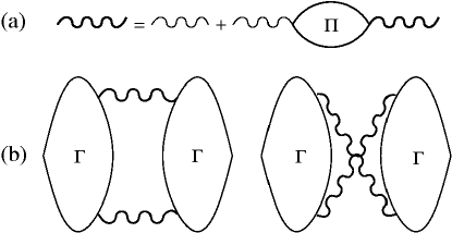
Figure 1: (a) Screened interlayer Coulomb interaction in the RPA. The thin and thick lines are the bare and the screened interactions, respectively. The bare bubble represents the polarizability $\Pi(q,\omega)$. (b) The leading order diagrams contributing to the drag conductivity. $\Gamma$ indicates the non-linear susceptibility.

The nonvanishing leading order diagrams corresponding to Eq. (14) are given in Fig. 1(b). The two leading order diagrams can be written in a symmetric form

$$\sigma_{D}(i\Omega_{n})=\frac{1}{2i\Omega_{n}}\frac{1}{T}\sum_{q,i\omega_{m}}\Gamma_{1}(q,\omega_{m}+\Omega_{n})\Gamma_{2}(q,\omega_{m})$$

$$\times V(q,\omega_{m}+\Omega_{n})V(q,\omega_{m}),$$ (15)

where $\Omega_{n}=2\pi inT$ and $\omega_{m}=2\pi imT$ are boson frequencies, $V(q,\omega)$ is the interlayer screened Coulomb interaction [Fig. 1(a)], and $\Gamma_{i}(q,\omega)$ is the three-point vertex diagrams (or the non-linear susceptibility) and given by flensberg:1995a ; kamenev:1995 ; tse:2007a

$$\Gamma(q,\omega)=T\sum_{\epsilon_{n}}{\rm Tr}\left\{G_{\epsilon_{n}}G_{\epsilon_{n}+\omega}J(q)G_{\epsilon_{n}+\omega}\right\}$$

$$+{\rm Tr}\left\{G_{\epsilon_{n}}G_{\epsilon_{n}-\omega}J(q)G_{\epsilon_{n}-\omega}\right\},$$ (16)

where $G_{\epsilon_{n}}$ is the Green function, $J(q)$ stands for the current and “Tr” the trace. To get the dc drag conductivity we need to perform an analytical continuation of external frequencies to a real value, $i\Omega_{n}\rightarrow\Omega$, and the limit $\Omega\rightarrow 0$ should be taken.

After summing over the boson frequencies, $\omega_{m}$, and performing an analytical continuation to a real value of $\Omega$ we have

$$\sigma_{D}=\frac{1}{16\pi T}\sum_{q}\int\frac{dw}{\sinh^{2}\frac{\omega}{2T}}\Gamma_{1}(q,\omega)\Gamma_{2}(q,\omega)\left|V(q,\omega)\right|^{2}.$$ (17)

The nonlinear susceptibility with real frequencies is given by

$$\Gamma(q,\omega) = \frac{1}{4\pi i}\int d\epsilon\left(\tanh\frac{\epsilon}{2T}-\tanh\frac{\epsilon}{2T}\right)$$ (18)

$$\times \sum_{p}{\rm Tr}\left[\left(G_{\epsilon}^{-}-G_{\epsilon}^{+}\right)G_{\epsilon+\omega}^{-}J(p)G_{\epsilon+\omega}^{+}\right]$$

$$+ \left\{(q,\omega)\rightarrow(-q,-\omega)\right\},$$

where $G_{\epsilon}^{\pm}=(\epsilon-H\pm i\gamma)^{-1}$ denotes the retarded ($-$) and advanced ($+$) Green function for a given system with the Hamiltonian $H$, respectively. Here we use a damping constant $\gamma=1/2\tau$ to include the disorder scattering in the Green function. In the Boltzmann regime ($\omega\tau\gg 1$ or $k_{F}l\gg 1$, where $k_{F}$ is the Fermi wave vector and $l=v_{F}\tau$ is the mean free path), which corresponds to weak impurity scattering and the actual experimental regime of the high mobility graphene samples, we can treat the vertex correction in the current $J(q)$ within the impurity ladder approximation kamenev:1995 ; tse:2007a . Then, the impurity-dressed current vertex becomes $J=(\tau_{tr}/\tau)\partial H/\partial k$, where $\tau_{tr}$ is the transport time. By using the following equation

$$G_{\epsilon+\omega}^{-}(p)G_{\epsilon+\omega}^{+}(p)=2\tau{\rm Im}G_{\epsilon+\omega}^{+}(p),$$ (19)

and expressing the matrix form of the Green function in the chiral basis, finally, we have the nonlinear susceptibility

$$\Gamma(q,\omega)=\tau\sum_{ss^{\prime},k}\left[J_{s}(k)-J_{s^{\prime}}(k+q)\right]F_{ss^{\prime}}(k,k+q)$$

$$\times{\rm Im}\frac{f_{sk}-f_{s^{\prime}k+q}}{\omega+\epsilon_{sk}-\epsilon_{s^{\prime}k+q}+i0^{+}}.$$ (20)

Comparing the above equation with Eq. (10) we have

$$\Gamma(q,\omega)=2{\rm Im}\chi(q,\omega).$$ (21)

Thus we recover the Boltzmann equation drag conductivity result by employing the leading order diagrammatic expansion within the Kubo formalism.

III Drag Resistivity in Monolayer Graphene

Monolayer graphene (MLG) is characterized by the presence of gapless linearly dispersing electron and hole bands with dispersion,

$$\epsilon_{s{\bf k}}=v_{F}k,$$ (22)

where $s=\pm 1$ denotes the electron and hole bands and $v_{F}$ is the Fermi velocity of graphene. The linear dispersion of MLG implies that the group velocity of the bands are given by $v_{s{\bf k}}=v_{F}{\bf k}/|{\bf k}|$. Thus, contrary to usual semiconductor systems, or the case of bilayer graphene to be treated later, the group velocity is constant in magnitude and does not scale with the momentum of the band-states. As we will show, this leads to profound qualitative differences in the variation of the MLG drag resistivity with the carrier densities in the layers and the distance between the layers. The chirality of the electrons (holes) are encoded in the band wavefunctions

$$\psi_{s{\bf k}}=\frac{1}{\sqrt{2}}\left(\begin{array}[]{c}e^{-i\theta_{\bf k}}\\ s\end{array}\right)$$ (23)

where $\theta_{\bf k}$ is the azimuthal angle in the 2D ${\bf k}$ space. This leads to the wavefunction overlap factor $F^{ss^{\prime}}_{{\bf k},{\bf q}}=(1/2)[1+ss^{\prime}\cos(\theta_{{\bf k}+{\bf q}}-\theta_{{\bf k}})]$.

Before we go on to a detailed discussion of the non-linear drag susceptibility and the drag resistivity in MLG, let us first discuss the finite temperature polarizability in MLG which will control the finite temperature screening of the Coulomb potential. Although analytic expressions for graphene polarizability at $T=0$ has been worked out beforehwang:2007 , the finite temperature versions of the polarizability have not been calculated analytically. The full expression of finite temperature polarizability is necessary to understand more precisely the temperature dependent drag including the plasmon enhancement effectsflensberg:1995 . Here we provide a finite temperature generalization of our earlier work on zero temperature graphene polarizability hwang:2007 . The MLG polarizability of layer $i$ is given by

$$\Pi_{i}(q,\omega,) = \frac{2E_{Fi}}{\pi v_{F}^{2}}\left(\frac{\pi}{8}\frac{y^{2}}{\sqrt{y^{2}-z^{2}}}\right.$$

$$+ \left.\int_{0}^{\infty}dx\left[f(x)+g(x)\right]\left[\frac{\left(\frac{z^{2}-y^{2}}{4}+zx+x^{2}\right){\rm sgn}(a_{+})}{\sqrt{\frac{(z^{2}-y^{2})^{2}}{4}+(z^{2}-y^{2})(zx+x^{2})}}+\frac{\left(\frac{z^{2}-y^{2}}{4}-zx+x^{2}\right){\rm sgn}(a_{-})}{\sqrt{\frac{(z^{2}-y^{2})^{2}}{4}+(z^{2}-y^{2})(-zx+x^{2})}}\right]\right),$$

where $x=k/k_{Fi}$, $y=q/k_{Fi}$ and $z=\omega/E_{Fi}$, $f(x)=[e^{-(x-\mu_{i})/t_{i}}-1]^{-1}$, $g(x)=[e^{(x+\mu_{i})/t_{i}}+1]^{-1}$, $a_{\pm}=z^{2}-y^{2}\pm 2zx$, with $E_{Fi}$ and $k_{Fi}$ being the Fermi energy and the Fermi wave-vector in layer $i$. Here, $\mu_{i}$ is the chemical potential in layer $i$ in units of $E_{Fi}$ (to be calculated self-consistently) and $t_{i}=T/E_{Fi}$.

We now turn our attention to the non-linear drag susceptibility and drag resistivity in MLG systems. The drag resistivity in MLG crucially depends on the variation of the transport scattering time with energy (or equivalently momentum). In this paper, we will consider the drag resistivity of MLG using two different models of scattering time: (a) a momentum independent scattering time $\tau_{{\bf k}}=\tau$ and (b) a scattering time scaling linearly with momentum (energy), $\tau_{\bf k}=\tau_{0}|{\bf k}|$, which results from the unusual screening of charge impurity potential in this linearly dispersive material novoselov:2005 ; tan:2007 ; chen:2008 ; dassarma:2011 .

We first consider the energy independent scattering time approximation. In this case, the non-linear drag susceptibility in MLG can be written as

$$\chi_{i}(q,\omega)=4\tau_{i}v_{F}\sum_{ss^{\prime}{\bf k}}\left(s\frac{{\bf k}+{\bf q}}{|{\bf k}+{\bf q}|}-s^{\prime}\frac{{\bf k}}{|{\bf k}|}\right)\frac{F^{ss^{\prime}}_{{\bf k},{\bf q}}(f^{i}_{s{\bf k}+{\bf q}}-f^{i}_{s^{\prime}{\bf k}})}{\omega-\varepsilon_{s{\bf k}+{\bf q}}+\varepsilon_{s^{\prime}{\bf k}}+i0^{+}}$$ (25)

Within the energy independent scattering time approximations, the intra-layer conductivities are given by $\sigma_{i}=e^{2}E_{Fi}\tau_{i}/4$.

We focus on the analytic asymptotic behaviors of the drag resistivity in MLG at low temperatures, both in the large layer separation weak coupling limit ($k_{F}d\gg 1$) and in the small layer separation strong coupling limit($k_{F}d\ll 1$). To calculate the asymptotic behavior of drag resistivity first we investigate the non-linear susceptibility for $\omega<v_{F}q<E_{F}$. Due to the phase-space restriction the most dominant contribution to the drag resistivity arises from $\omega<v_{F}q$ at low temperatures. When we neglect the energy dependence in the transport times, i.e., $\tau_{k}=\tau$, then we obtain, for $\omega<v_{F}q$,

$$\chi(q,\omega)\sim\frac{\tau q^{2}}{\pi E_{F}}\frac{\omega}{v_{F}q}\sqrt{1-{q^{2}}/{4k_{F}^{2}}}.$$ (26)

With assumptions of a large inter-layer separation ($k_{F}d\gg 1$, or $q_{TF}d\gg 1$, with $q_{TF}$ being the Thomas Fermi (TF) screening wave vector) and the random phase approximation (RPA) in which $\Pi_{ii}$ is replaced by its value for the non-interacting electrons, we have the drag resistivity at high density and low temperature,

$$\rho_{D}=\frac{h}{e^{2}}\frac{5!\zeta(5)}{3\cdot 2^{8}}\frac{(k_{B}T)^{2}}{E_{F_{1}}E_{F_{2}}}\frac{1}{(q_{TF_{1}}d)(q_{TF_{2}}d)(k_{F_{1}}d)^{2}(k_{F_{2}}d)^{2}}$$ (27)

where $q_{TF}=4r_{s}k_{F}$ is the TF wave vector with the graphene fine structure constant $r_{s}=e^{2}/\kappa v_{F}$ and $\zeta(x)$ is the Riemann zeta function. This result shows that $\rho_{D}(n)\propto n^{-4}$ and $\rho_{D}(T)\propto T^{2}$. For large layer separation (i.e. $k_{F}d\gg 1$) the back-scattering $q\approx 2k_{F}$ is suppressed due to the exponential dependence of the interlayer Coulomb interaction $v_{12}(q)\propto\exp(-qd)/q$ as well as the graphene chiral property. In this case the drag is dominated by small angle scattering and one expects $\rho_{D}\propto T^{2}/(n^{4}d^{6})$.

For the strong interlayer correlation ($k_{F}d\ll 1$) in the low-density or small-separation limit, the asymptotic behavior behavior of drag resistivity becomes

$$\rho_{D}=\frac{h}{e^{2}}\frac{1}{6}\frac{(k_{B}T)^{2}}{E_{F_{1}}E_{F_{2}}}\frac{r_{s}^{2}}{(k_{F_{1}}d)(k_{F_{2}}d)}.$$ (28)

We have the same temperature dependence, $\rho_{D}(T)\sim T^{2}$, but the density dependence becomes much weaker, $\rho_{D}(n)\sim 1/(nd)^{2}$. At low densities (or strong interlayer correlation, $k_{F}d\ll 1$) the exponent in the density dependent drag differs from -4. In an ordinary 2D systems, at low carrier densities and for closely spaced layers the backward scattering can be important since $k_{F}d\sim 1$. In the low temperature range $T/T_{F}\ll 1$ the enhanced phase space for $q=2k_{F}$ backward Coulomb scattering leads to $\ln(T)$ corrections to the usual $T^{2}$ dependence of the drag, i.e. $\rho_{D}\propto T^{2}\ln T$. However, due to the suppression of the $q=2k_{F}$ back-scattering due to the chirality of graphene there is no $\ln(T)$ correction in the drag resistivity of monolayer graphene.

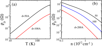
Figure 2: The calculated drag resistivity by considering the energy independent scattering approximation. (a) The temperature dependence of Coulomb drag for two different layer separations $d=50$Å, $d=100$Å  and the equal electron densities, $n_{1}=n_{2}=10^{12}cm^{-2}$. (b) The density dependent Coulomb drag for different layer separations $d=5$, 10, 20 nm and at $T=200K$.

The drag resistivity within this approximation is plotted as a function of temperature and density in Fig. 2 for different layer separations. The parameters corresponding to the experimental setup of ref. kim:2011, are used. In Fig. 2(a) we show the calculated Coulomb drag as a function of temperature for an equal carrier density, $n_{1}=n_{2}=10^{12}cm^{-2}$, for two different layer separations $d=50$ Å and $d=200$ Å. The overall temperature dependence of drag is close to the quadratic behavior, $\rho_{D}\propto T^{2}$. But we find a small corrections at low temperatures, especially at low values of $k_{F}d$. In regular 2D systems there is a $\ln(T)$ corrections to the $T^{2}$ dependence of the drag. However, due to the suppression of the back-scattering in graphene such logarithmic correction does not show up in our numerical results except perhaps at extremely low temperatures. In Fig. 2 (b) the density dependent Coulomb drag is shown for different layer separations. Our calculated Coulomb drag resistivity follow a $n^{\alpha}$ dependence with $\alpha\sim-2$ at low carrier densities (or, $k_{F}d<1$), but as the density increases the exponent decrease to $\alpha\sim-4$.

So far, we have considered the energy independent scattering time. However, it is known that the scattering by the charged impurity disorder which inevitably exist in the graphene environment dominates and the scattering time due to the charged impurity is linearly proportional to the energy, $\tau_{i}\sim\varepsilon=\tau^{0}_{i}k$. novoselov:2005 ; tan:2007 ; chen:2008 ; dassarma:2011 . In this approximation, the nonlinear drag susceptibility is given by

$$\chi_{i}(q,\omega)=4\tau^{0}_{i}v_{F}\sum_{ss^{\prime}{\bf k}}[s({\bf k}+{\bf q})-s^{\prime}{\bf k}]\frac{F^{ss^{\prime}}_{{\bf k},{\bf q}}(f^{i}_{s{\bf k}+{\bf q}}-f^{i}_{s^{\prime}{\bf k}})}{\omega-\varepsilon_{s{\bf k}+{\bf q}}+\varepsilon_{s^{\prime}{\bf k}}+i0^{+}}$$ (29)

In this case, we will mainly focus on the low temperature asymptotic for of the drag resistivity. For linearly energy dependent scattering time due to the charged impurities, the non-linear susceptibility for $w<v_{F}q$ is

$$\chi_{i}(q,\omega)=\frac{2\tau^{0}_{i}}{\pi}\frac{k_{F}}{v_{F}}\frac{\omega}{E_{F}}\frac{1}{\sqrt{1-q^{2}/4k_{F}^{2}}}.$$ (30)

Then the drag resistivity for a large inter-layer separation ($k_{F}d\gg 1$) is given by

$$\rho_{D}=\frac{h}{e^{2}}\frac{\zeta(3)}{2^{3}}\frac{(k_{B}T)^{2}}{E_{F_{1}}E_{F_{2}}}\frac{1}{(k_{F_{1}}d)(k_{F_{2}}d)(q_{TF_{1}}d)(q_{TF_{2}}d)},$$ (31)

and for the strong interlayer correlation limit ($k_{F}d\ll 1$), we have

$$\rho_{D}=\frac{h}{e^{2}}\frac{2^{4}r_{s}^{2}}{3}\frac{(k_{B}T)^{2}}{E_{F_{1}}{E_{F_{2}}}}\ln\left[\frac{2(q_{TF_{1}}+q_{TF_{2}})d+1}{2(q_{TF_{1}}+q_{TF_{2}})d}\right].$$ (32)

Thus we see that when we consider the energy dependent intralayer scattering time we have very different asymptotic behaviors compared to the results from energy independent scattering time, i.e., we find for $k_{F}d\gg 1$, $\rho_{D}\sim T^{2}/(n^{3}d^{4})$ and for $k_{F}d\ll 1$, $\rho_{D}\sim T^{2}\ln(\sqrt{n}d)$. Thus in the presence of the strong charged impurity scattering the Coulomb drag resistivity follow a $n^{\alpha}$ dependence with $\alpha\lesssim-3$ at high densities but as the density decreases the exponent ($\alpha$) increase. Based on our calculation we believe that the experimental departure from the $n^{-3}$ behavior reported in Ref. kim:2011 is essentially a manifestation of the fact that the asymptotic $n^{-3}$ regime is hard to reach in low density electron systems where $k_{F}d\gg 1$ limit simply cannot be accessed. We predict a weak $\ln(n)/n$ density dependence in the low-density or small separation limit.

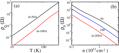
Figure 3: The calculated drag resistivity by considering the linearly energy dependent scattering time. (a) The temperature dependence of Coulomb drag for two different layer separations $d=50$Å, $d=200$Å  and the equal electron densities, $n_{1}=n_{2}=10^{12}cm^{-2}$. (b) The density dependent Coulomb drag for different layer separations $d=5$, 10, 20 nm and at $T=200K$.

In Fig. 3(a) we show the calculated Coulomb drag as a function of temperature for two different layer separation (a) $d=50$ Å (b) $d=100$ Å by considering the linearly energy dependent scattering time. The overall temperature dependence of drag increases quadratically and there is no logarithmic correction due to the suppression of the back-scattering. In Fig. 3(b) the density dependent Coulomb drag is shown for different layer separations. The density dependent Coulomb drag follow a $n^{\alpha}$ dependence with $\alpha\sim-2$. Based on our calculation the consideration of the energy dependent scattering time is crucial to understand experiment measurements of Ref. kim:2011, .

IV Drag Resistivity in Bilayer Graphene

In this section we will study the drag resistance in a heterostructure made of two bilayer graphene (BLG) layers separated by an insulating barrier and study its dependence on temperature, density and separation of the layers. Both BLG and MLG have chiral gapless electron and hole bands. However, BLG differs from MLG in two crucial aspects: (i) the bands have a parabolic dispersion as opposed to linear dispersion in MLG and (ii) the chiral angle is double that in MLG leading to enhanced rather than suppressed backscattering between the quasiparticles. We will show in this section how these two differences lead to dramatic changes in the density and layer separation dependence of the BLG drag resistivity compared to MLG drag resistivity.

BLG consists of an electron and a hole band with quadratic dispersion

$$\epsilon_{s{\bf k}}=sk^{2}/2m$$ (33)

($s=\pm 1$ for electron(hole) band) and the BLG mass is $m=0.033m_{e}$, where $m_{e}$ is the electron mass. The group velocity in the two bands are ${\bf v}_{s{\bf k}}=s{\bf k}/m$, which scales linearly with momentum. The wavefunctions in these bands are given by

$$\psi_{s{\bf k}}=\frac{1}{\sqrt{2}}\left(\begin{array}[]{c}e^{-2i\theta_{\bf k}}\\ s\end{array}\right)$$ (34)

which gives the overlap factor $F^{ss^{\prime}}_{{\bf k},{\bf q}}=(1/2)(1+ss^{\prime})-ss^{\prime}q^{2}\sin^{2}\phi/|{\bf k}+{\bf q}|^{2}$, where $\phi$ is the angle between ${\bf k}$ and ${\bf q}$.

Without loss of generality, we will assume that the applied electric field, the induced electric field and the resultant currents are all in the $\hat{x}$ direction. We will also assume that the chemical potential in both layers is in the conduction (electron) band, i.e. they are electron doped. The chemical potential as a function of temperature is obtained by solving the integral equation

$$g\sum_{{\bf k}}\frac{1}{e^{(k^{2}/2m-\mu_{i})/T}+1}+\frac{1}{e^{-(k^{2}/2m+\mu_{i})/T}+1}-1=\rho_{i}$$ (35)

where $\rho_{i}$ is the density of the layer $i$. It is an interesting feature of the BLG dispersion that in the non-interacting approximation, the chemical potential is independent of the temperature and is given by $\mu_{i}=E_{fi}$, where $E_{fi}$ is the Fermi energy of the electrons in layer $i$.

We will first focus on the polarizability and hence the screened Coulomb interaction in BLG systems. The analytic form for the BLG polarizability at zero temperature has been derived before sensarma:2010 , but we need to take into account the temperature dependence of the screening to study the detailed behaviour of the drag resistivity with temperature. Here, we generalize our earlier results on BLG polarizability to finite temperature. The polarizability can be broken up into the intra-band [$s=s^{\prime}$ terms in Eq. (13)] and inter-band [$s\neq s^{\prime}$ terms in Eq. (13)] contributions. Working out the azimuthal integrals analytically we obtain

$$\Pi_{i}^{intra}({\bf q},\omega)=\frac{gm}{4\pi}\int_{0}^{\infty}dx\frac{(f^{i}_{+x}-f^{i}_{-x})}{x(x^{2}+z)}\left[|x^{2}-y^{2}|-(x^{2}+z)+sgn(\zeta_{1}+2xy)\frac{(2x^{2}+\zeta_{1})^{2}}{\sqrt{\zeta_{1}^{2}-4x^{2}y^{2}}}\right]+(y,z\rightarrow-y,-z)$$ (36)

and

$$\Pi_{i}^{inter}({\bf q},\omega)=-\frac{gm}{4\pi}\int_{0}^{\infty}dx\frac{(f^{i}_{+x}-f^{i}_{-x})}{x(x^{2}+z)}\left[|x^{2}-y^{2}|+(x^{2}+z)-sgn(\zeta_{2}+2xy)\sqrt{\zeta_{2}^{2}-4x^{2}y^{2}}\right]+(y,z\rightarrow-y,-z)$$ (37)

where $y=q/k_{Fi}$, $x=k/k_{Fi}$, $z=\omega/E_{Fi}$, $\zeta_{1}=z-y^{2}$, $\zeta_{2}=z+2x^{2}+y^{2}$, and $f_{sx}=1/(e^{(sx^{2}-1)/t_{i}}+1)$ with $t_{i}=T/E_{Fi}$

We will now shift our attention to the non-linear drag susceptibility. For BLG systems, both charge impurity scattering and short range impurity scattering leads to a transport scattering time independent of momenta, and hence, we will only consider an energy independent scattering time, $\tau^{i}_{{\bf k}}=\tau^{i}$, in this case. With this approximation the nonlinear drag susceptibility is given by

$$\chi_{i}(q,\omega)=\frac{4\tau_{i}}{m}\sum_{ss^{\prime}{\bf k}}[s({\bf k}+{\bf q})-s^{\prime}{\bf k}]\frac{F^{ss^{\prime}}_{{\bf k},{\bf q}}(f^{i}_{s{\bf k}+{\bf q}}-f^{i}_{s^{\prime}{\bf k}})}{\omega-\varepsilon_{s{\bf k}+{\bf q}}+\varepsilon_{s^{\prime}{\bf k}}+i0^{+}}$$ (38)

where $m$ is the BLG mass. $m=0.033m_{e}$, where $m_{e}$ is the free electron mass.

The non-linear susceptibility $\chi^{x}_{i}$ can be separated into an intra-band contribution and an inter-band contribution. The azimuthal integrals can be done analytically and we get

$$Im[\chi^{x(intra)}_{i}(q,\omega)]=\frac{\tau^{i}k_{Fi}y\cos\phi_{q}}{\pi}\left[\int_{\frac{|z-y^{2}|}{2y}}^{\infty}dx\frac{f^{i}_{+x}+f^{i}_{-x}}{x(x^{2}+z)}\frac{(2x^{2}+z-y^{2})^{2}}{\sqrt{4x^{2}y^{2}-(z-y^{2})^{2}}}-(z\rightarrow-z)\right]$$ (39)

and

$$\displaystyle Im[\chi^{x(inter)}_{i}(q,\omega)]=\frac{\tau^{i}k_{Fi}\cos\phi_{q}}{\pi y}\left[\Theta(b)\int_{\frac{|y-\sqrt{b}|}{2}}^{\frac{|y+\sqrt{b}|}{2}}dx\frac{f^{i}_{+x}+f^{i}_{-x}}{x(x^{2}-z)}(2x^{2}-z)\sqrt{4x^{2}y^{2}-(2x^{2}+y^{2}-z)^{2}}-(z\rightarrow-z)\right]$$ (40)

where $b=2z-y^{2}$ and $\phi_{q}$ is the azimuthal angle related to the vector ${\bf q}$.

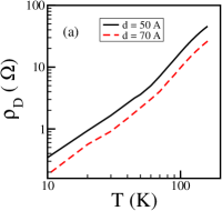
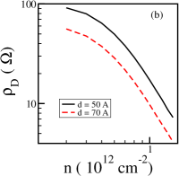
Figure 4: (a): The Coulomb drag resistivity in BLG as a function of temperature for two layer separations, $d=50\AA$ (thick black line) and $d=70\AA$ (dashed red line). The density of the two layers $n_{1}=n_{2}=10^{12}cm^{-2}$. (b): The density dependence of bilayer Drag at a temperature $T=100K$. The thick black line is for $d=50\AA$ and the dashed red line is for $d=70\AA$. We have used a dielectric constant $\kappa=4$ corresponding to boron nitride substrate

We note that the intra-band drag susceptibility is proportional to the intra-band polarizability of BLG ($\chi^{intra}({\bf q},\omega)=(4\tau/m){\bf q}\Pi^{intra}({\bf q},\omega)$) only in the $T=0$ limit. This relation breaks down at finite temperatures. Finally, with a momentum independent scattering time, and a quadratic dispersion, the intra-layer conductivity can be written in the simple form $\sigma^{i}=n_{i}e^{2}\tau^{i}/m$. Note that the scattering times cancel in the expression for drag resistivity which is purely dominated by electron-electron interactions. In figure 4 (a), we plot the temperature dependence of the BLG drag resistivity for two different layer separations with a common layer carrier density of $n_{1}=n_{2}=10^{12}cm^{-2}$. The drag shows a quadratic behaviour with logarithmic corrections at low temperatures. In figure 4(b), we plot the density dependence of the bilayer drag at $T=100K$ for two different layer separations.

We now focus on the low temperature asymptotic behaviour of the BLG drag resistivity. To obtain the leading temperature dependence of $\rho_{D}$ at low temperatures, both $\chi$ and $\Pi$ can be replaced by their intra-band contributions at $T=0$ in the limit of small $q,\omega$, i.e. $Im[\chi^{i}(q,\omega)]\sim(gm/2\pi)\tau_{i}\omega/k_{F}$, and the screened Coulomb interaction is replaced by its static value with $\Pi_{1}=\Pi_{2}\sim gm/(2\pi)$. The screening in BLG is controlled by the Thomas-Fermi wave-vector $q_{TF}=e^{2}gm/\kappa$, where $\kappa$ is the background dielectric constant. For large layer separation, i.e. $q_{TF}d\gg 1$, the screened interaction has the form $V(q)\sim q/[D_{0}q_{TF}\sinh(qd)]$ in which $D_{0}=gm/2\pi$ is the density of states of bilayer graphene at Fermi level, and the leading order drag-resistivity is given by

$$\rho_{D}\sim\frac{1}{e^{2}}\frac{\pi^{2}\zeta(3)}{16}\frac{T^{2}}{E_{F1}E_{F2}}\frac{1}{(k_{F1}d)(k_{F2}d)(q_{TF}d)^{2}}.$$ (41)

We note that contrary to MLG, $q_{TF}$ in BLG is a constant and is independent of the density. Thus the large layer separation limit is not the same as the high density limit ($k_{F}d\gg 1$). In the opposite limit of small layer separation ($q_{TF}d\ll 1$) and strong interlayer correlations, the screened interaction takes the form $V(q)\sim(q_{TF}/D_{0})exp(-qd)/(q+2q_{TF})$ and the leading order drag resistivity is given by

$$\rho_{D}\sim\frac{1}{e^{2}}\frac{\pi^{2}}{24}\frac{T^{2}}{E_{F1}E_{F2}}\frac{q_{TF}^{2}}{k_{F1}k_{F2}}[-\ln q_{TF}d+\gamma-1-\ln 4+...],$$ (42)

where $\gamma$ is the Euler constant. Thus the drag resistance $\sim T^{2}$ both in the large and small layer separation limit. The density dependence of the coefficient of the $T^{2}$ term is $1/(n_{1}n_{2})^{3/2}$ in both limits. In the large separation limit, the leading order term $\sim 1/d^{4}$, whereas in the small separation limit, the drag resistivity shows a weak logarithmic dependence on the layer separation. We also note that, since backscattering is enhanced in BLG, there will be an additional $T^{2}\ln T$ correction to the formulae derived here.

V Conclusion

In this paper, we have theoretically studied the frictional drag between two spatially separated MLG and BLG layers to lowest nonvanishing order in the screened interlayer electron-electron interaction using Boltzmann transport theory (which is equivalent to a leading-order diagrammatic perturbation theory). We find that the low temperature drag mostly shows a quadratic temperature dependence, both in MLG and BLG, regardless of the layer separation and density of carriers. However the density and layer separation dependence of the coefficient of the $T^{2}$ term is very different for MLG and BLG.

The density and layer separation dependence of low temperature MLG drag resistivity crucially depends on the variation of the intralayer momentum scattering time with energy. For energy independent intralayer scattering time (which does not correspond to any model of disorder in MLG, but captures the effects of both short range and screened Coulomb impurities in standard 2DEG), the drag varies from $\rho_{D}\propto T^{2}/(nd)^{2}$ for $k_{F}d\ll 1$ to $\rho_{D}\propto T^{2}/(n^{4}d^{6})$ for $k_{F}d\gg 1$. However, for energy dependent intralayer scattering times (corresponding to intralayer Coulomb scattering by random charged impurities in the environment) the power law of density dependence is significantly changed. Thus, an accurate measurement of interlayer MLG drag is in principle capable of distinguishing the main disorder scattering. In most currently available graphene samples the scattering due to charged impurity disorder dominates. In this case the intralayer scattering time depends linearly on the energy and the drag resistivity becomes $\rho_{D}\propto\ln(\sqrt{n}d)/n$ for $k_{F}d\ll 1$ and $\rho_{D}\propto n^{-3}d^{-4}$ for $k_{F}d\gg 1$. We note that the density dependence of drag resistivity is very sensitive to the experimental setup, so the density dependence does not have any universal power law behavior because one is never in any asymptotic regime with clear cut analytical power law behavior. Experimental measurementskim:2011 therefore may not find any clear cut power law behavior in the density dependence of MLG drag since one is always in the crossover regime. We also find that due to the suppression of the $q=2k_{F}$ back-scattering in graphene there are no $\sim T^{2}\ln(T)$ corrections to the low temperature MLG drag resistivity.

We would like to take this opportunity to compare this work, which is a more complete and updated version of ref. hwang_sds:drag, , with recent works on low temperature MLG drag resistivitytse:2007 ; narozhny:2007 ; peres:2011 ; katsnelson:2011 , which predict widely varying density and layer separation dependence of the low temperature MLG drag resistivity. Within energy independent scattering time approximation, Tse et al. tse:2007 studied the drag in MLG in the high density limit and obtained $\rho_{D}\sim T^{2}/n^{3}d^{4}$. Katsnelson katsnelson:2011 also obtained the same result in the high density limit ($k_{F}d\gg 1$) and additionally considered the $k_{F}d\ll 1$ limit of ref. tse:2007, finding a $\rho_{D}\sim T^{2}\ln(nd^{2})/n$ dependence in the low density limit. Narozhny narozhny:2007 , on the other hand, found that the drag vanishes for linearly dispersive Dirac particles. In the current paper, within the energy independent scattering time approximation, we find that $\rho_{D}\sim T^{2}/n^{4}d^{6}$ in the high density limit and $\rho_{D}\sim T^{2}/n^{2}d^{2}$ in the low density limit. Narozhny narozhny:2007 computes the drag to linear order in the inter-layer potential where it is known to vanish even for ordinary 2D electron systems. The drag resistivity is at least quadratic in the inter-layer potential and its vanishing to linear order is a rather trivial result. The main difference between our present work and Ref. tse:2007, and  katsnelson:2011, arises because both these papers use a form of the non-linear drag susceptibility where the band group velocity scales linearly with the momentum $k$ and results in a leading order $q$ dependence of the vertex in the susceptibility. While this is true for quadratic band dispersions as in regular 2D and BLG systems, the group velocity in linearly dispersive MLG is constant in magnitude($v_{F}$), and combined with the overlap functions, gives rise to a leading order $q^{2}$ momentum in the non-linear susceptibility in our case. This accounts for the discrepancy between our results and earlier results.

Finally Peres et. al peres:2011 considers the drag resistivity of MLG within a linearly energy dependent scattering time approximation and obtains $\rho_{D}\sim T^{2}/n^{4}d^{6}$ in the high density limit and $\rho_{D}\sim T^{2}/n^{2}d^{2}$ in the low density limit. These results match with our energy independent scattering time approximation results, whereas within linearly energy dependent scattering time, we get $\rho_{D}\sim T^{2}/n^{3}d^{4}$ in the high density limit and $\rho_{D}\sim T^{2}\ln(nd^{2})/n$ in the low density limit. This discrepancy can also be understood in terms of the scaling of the current vertex factors. The vertex factor going into the drag susceptibility is $v_{s{\bf k}}\tau_{\bf k}$. Peres et. al peres:2011 uses a drag susceptibility where the vertex factor in the susceptibility scales as $q^{2}$. Thus they recover our energy independent scattering time scaling. However, with a constant group velocity, as is the case for MLG, the energy dependent scattering time approximation should lead to a leading order $q$ dependence (coming from the momentum dependence of the scattering time) of the vertex and this accounts for the discrepancy between our results and Peres et. al. The conceptual element of our work is the new role of group velocity in the nonlinear susceptibility defining the drag, which turns out to be crucial to the calculation of Coulomb drag in monolayer graphene (with its linear energy-momentum dispersion). We have also studied the drag resistivity in two spatially separated bilayer-graphene structures. We find that the drag resistivity shows a quadratic temperature dependence at low temperatures, as for monolayer graphene. The density dependence of the BLG drag is independent of the layer separation with $\rho_{D}\propto T^{2}/n^{3}$ both in the large and small layer separation limit. In the large layer separation limit (weak inter-layer correlation), the drag has a strong $1/d^{4}$ dependence on layer separation, whereas this goes to a weak logarithmic dependence in the strong inter-layer correlation limit.

References

- (1) S. Das Sarma, S. Adam, E. H. Hwang, and E. Rossi, Rev. Mod. Phys. 83, 407 (2011)
- (2) S. Kim, I. Jo, J. Nah, Z. Yao, S. K. Banerjee, and E. Tutuc, Phys. Rev. B 83, 161401 (2011)
- (3) B. E. Feldman, J. Martin, and A. Yacoby, Nature Phys. 5, 889 (2009)
- (4) H. Min, G. Borghi, M. Polini, and A. H. MacDonald, Phys. Rev. B 77, 041407 (2008)
- (5) E. H. Hwang and S. Das Sarma, Phys. Rev. B 80, 205405 (2009)
- (6) R. Nandkishore and L. Levitov, Phys. Rev. Lett. 104, 156803 (2010)
- (7) T. J. Gramila, J. P. Eisenstein, A. H. MacDonald, L. N. Pfeiffer, and K. W. West, Phys. Rev. Lett. 66, 1216 (1991)
- (8) L. Zheng and A. H. MacDonald, Phys. Rev. B 48, 8203 (1993)
- (9) K. Flensberg and B. Y.-K. Hu, Phys. Rev. B 52, 14796 (1995)
- (10) A. G. Rojo, J. Phys.: Condens. Matter 11, R31 (1999)
- (11) E. H. Hwang, S. Das Sarma, V. Braude, and A. Stern, Phys. Rev. Lett. 90, 086801 (2003)
- (12) S. Das Sarma and E. H. Hwang, Phys. Rev. B 71, 195322 (2005)
- (13) W.-K. Tse, B. Y.-K. Hu, and S. Das Sarma, Phys. Rev. B 76, 081401 (2007)
- (14) K. S. Novoselov et al., Nature 438, 197 (2005)
- (15) Y.-W. Tan, Y. Zhang, K. Bolotin, Y. Zhao, S. Adam, E. H. Hwang, S. Das Sarma, H. L. Stormer, and P. Kim, Phys. Rev. Lett. 99, 246803 (2007)
- (16) J. H. Chen, C. Jang, M. S. Fuhrer, E. D. Williams, and M. Ishigami, Nature Phys. 4, 377 (2008)
- (17) K. Flensberg, B. Y.-K. Hu, A.-P. Jauho, and J. M. Kinaret, Phys. Rev. B 52, 14761 (1995)
- (18) A. Kamenev and Y. Oreg, Phys. Rev. B 52, 7516 (1995)
- (19) W.-K. Tse and S. Das Sarma, Phys. Rev. B 75, 045333 (2007)
- (20) E. H. Hwang and S. Das Sarma, Phys. Rev. B 75, 205418 (2007)
- (21) R. Sensarma, E. H. Hwang, and S. Das Sarma, Phys. Rev. B 82, 195428 (2010)
- (22) E. H. Hwang and S. D. Sarma, arXiv:1105.3203(2011)
- (23) B. N. Narozhny, Phys. Rev. B 76, 153409 (2007)
- (24) N. M. R. Peres, J. M. B. Lopes dos Santos, and A. H. Castro Neto, arXiv:1105.5399; Europhys. Lett. 95, 18001 (2011)
- (25) M. I. Katsnelson, arXiv:1105.2534; Phys. Rev. B 84, 041407 (2011)