Deriving the Rosenfeld Functional from the Virial Expansion

Abstract

In this article we replace the semi-heuristic derivation of the Rosenfeld functional of hard convex particles with the systematic calculation of Mayer clusters. It is shown that each cluster integral further decomposes into diagrams of intersection patterns that we classify by their loop number. This extends the virial expansion of the free-energy by an expansion in the loop order, with the Rosenfeld functional as its leading contribution. Rosenfeld’s weight functions then follow from the derivation of the intersection probability by generalizing the equation of Blaschke, Santalo, and Chern. It is found that the 0-loop order can be derived exactly and reproduces the Rosenfeld functional. We further discuss the influence of particle dimensions, topologies, and geometries on the mathematical structure of the calculation.

I Introduction

Hard particle systems serve as reference fluids for soft, granular, and cellular matter. They interpolate the phase diagrams of molecular particles in the limits of low and high particle densities, where the influence of the smooth and attractive interactions is of secondary order. Phase transitions, as nematic and smectic, can be understood as entropic effects of the excluded volume hard-sphere-rev . This distinguishes hard particle systems as the ideal starting point for perturbation theory. However, it also requires an analytic representation, or at least detailed knowledge, of the free-energy functional. This requirement limits the usefulness of computer simulations, as the minimization procedure needs the functional form of the free-energy and not its function. To obtain a theoretical understanding of the liquid, crystalline, amorphous, and glassy states stillinger we therefore need better analytical tools than are currently available.

During the last decades, several interesting approximations have been developed to derive analytical expressions of the free-energy or the pair-correlation function mcdonald . However, most of them are restricted to hard spheres, such as the well known solution of Thiele and Wertheim thiele ; wertheim-py1 ; wertheim-py2 of the Ornstein-Zernicke equation in the Percus-Yevick approximation. A different approach was suggested by Reiss, Frisch, and Lebowitz scaled-particle-1 , who used the result of Isihara and Kihara isihara-orig ; kihara-1 ; kihara-2 for the second virial coefficient for convex particles. Their scaled particle theory motivated Rosenfeld rosenfeld-structure ; rosenfeld-freezing ; rosenfeld-closure ; rosenfeld-mixture ; rosenfeld1 to develop the fundamental measure theory, which is based on the local decoupling of the second virial integral, on the invariance of the free-energy functional under coordinate rescaling and on its solution of the scaled particle differential equation. The Rosenfeld functional is therefore a semi-heuristic result, valid under the same assumptions as the scaled particle theory. Nevertheless, its advantage is the explicit dependence on the particle geometry through the weight functions and its local representation of the free-energy functional as the convolute of weight densities.

Later it has been shown by Rosenfeld and Tarazona tarazona-rosenfeld ; tarazona ; crossover-rosenfeld-1 ; crossover-ros-1 ; crossover-rosenfeld-2 that the functional leads to an inconsistency when the volume, filled with spheres, is restricted to a single layer, a tube or a one-particle cavern. This led to a geometrically motivated correction of the original form and resulted in a highly accurate functional for the fluid phase of hard spheres up to the freezing point tarazona ; comparision-ros . A different strategy made use of simulation data to go beyond the Percus-Yevick approximation white-bear-1 ; white-bear-2 . The simple structure of the functional led to further applications for cylinders, discs, needles, and their mixtures schmidt-dft ; schmid-c ; schmidt-mixtures ; schmidt-colloidal ; schmidt-one-dim ; schmidt-palelet ; goos-mecke and alternative representations of the weight functions rosinberg-kierlik-1 ; rosinberg-kierlik-2 . For a recent review see also roth_rev . However, despite its success, it is not clear, how to extend Rosenfeld’s approach further and how to go beyond the semi-heuristic construction of the functional.

In this article we will begin an investigation to clarify the underlying mathematical and physical assumptions of the fundamental measure theory. In a first step it will be shown that the Rosenfeld functional is only the leading order of an infinite expansion of the free-energy in intersection diagrams, which will be classified by their number of loops and intersection centers. The 0-loop order corresponds to sets of particles that intersect in at least one common point and can freely rotate around this center. This intersection pattern corresponds to an infinite subset of Mayer clusters and will be derived in this work by generalizing the equation of Blaschke, Santalo, and Chern blaschke ; santalo-book ; chern-1 ; chern-2 ; chern-3 . It will be shown that the infinite number of terms of the 0-loop contribution requires only the calculation of three Euler forms. The relation between the intersection probabilities and their corresponding subsets of Mayer clusters then allows the calculation of the free-energy functional via the virial expansion. However, instead of the virial series in the single-particle density, we have to interpret the expansion in Rosenfeld’s weight densities. This reformulation of the virial expansion not only reproduces the Rosenfeld functional as the 0-loop order but applies also to all further loop orders.

The article is divided into two sections. The scope of part II is more general. Here, we introduce the concept of the loop expansion, II.1, give some background information on differential and integral geometry, II.2, and lastly derive the weight functions from integral geometry in section II.3. Part III considers the 0-loop contribution of the free-energy. III.1 recapitulates Rosenfeld’s ideas leading to the semi-heuristic formulation of the fundamental measure theory and Tarazona’s corrections. This approach is compared in III.2 to our new ansatz via the virial expansion, where we derive the 0-loop contribution of the free-energy and prove its equivalence to Rosenfeld’s functional. We end the article in IV with a discussion of the convergence of the loop expansion.

II The Intersection Probability of Particle Stacks

II.1 Intersecting Particle Stacks

So far, little attention has been paid to the approximation scheme leading to Rosenfeld’s free-energy functional. Instead, fundamental measure theory is based on a tower of three postulates that fix the functional’s overall structure: 1. the free-energy functional density is assumed to be a polynomial in weight densities, 2. uniquely determined by its the homogeneous scaling dimension and 3. its solution of the empirical scaled particle differential equation. Actually, there is no physical argument that justifies these assumptions from first principles, and the failure of only one postulate could cause the downfall of the remaining parts. A first step in generalizing Rosenfeld’s approach is therefore to test these three postulates and, if necessary, to replace them. This will be done in the following by comparing the third virial order of Rosenfeld’s functional to its exact integral.

Rosenfeld’s truly remarkable step in developing a weighted density functional for spheres is the local splitting of Mayer’s f-function into weight functions and to recognize its relation to the Gauss-Bonnet equation and thus to the Gaussian curvature $K$ rosenfeld-structure ; rosenfeld2 ; rosenfeld-gauss2 . For two particles $D_{i},D_{j}$, intersecting in a domain $A=D_{i}\cap D_{j}$ of coordinate vector $\vec{r}_{A}\in D_{i}\cap D_{j}$, the f-function decouples into the convolute

$$f_{ij}(\vec{r}_{ij})=-\frac{1}{4\pi}\int_{\partial(D_{i}\cap D_{j})}K(A)\,dS_{A}$$

$$\qquad\quad\,=-\frac{1}{4\pi}\int_{D_{i}\cap D_{j}}\quad K(A)\,\delta(\vec{n}\vec{r}_{A})\,d^{3}r_{A}$$ (1)

$$=\int_{D_{i}\cap D_{j}}C^{A_{1}A_{2}}\omega^{i}_{A_{1}}(\vec{r}_{A})\omega^{j}_{A_{2}}(\vec{r}_{A}-\vec{r}_{ij})\,d^{3}r_{A}$$

$$=\int_{D_{i}\cap D_{j}}C^{A_{1}A_{2}}\omega^{i}_{A_{1}}(\vec{r}_{A}-\vec{r}_{i})\omega^{j}_{A_{2}}(\vec{r}_{A}-\vec{r}_{j})\,d^{3}r_{A}$$ (2)

depending on the particle positions $\vec{r}_{i}\in D_{i}$, $\vec{r}_{j}\in D_{j}$ and the distance vector $\vec{r}_{ij}=\vec{r}_{j}-\vec{r}_{i}$. In (1) the integration over the surface $S_{A}$ has been transformed into a volume integral at normal vector $\vec{n}$ by equation (134) and finally arranged in the symmetric form (2), assuming that the embedding space of the particles is of infinite volume.

The derivation of the local decoupling of the f-function (2) and its relationship to the Gauss-Bonnet equation will be explained in the following sections and deduced from the Blaschke, Santalo, Chern equation of integral geometry blaschke ; santalo-book ; chern-1 ; chern-2 . It provides an exact identity for the intersection probability of convex particles and determines the pre-factor $1/(4\pi)$ uniquely. Based on this result, any Mayer diagram can be transferred into weight functions.

The third virial cluster in this representation is now an integral over three intersection centers $A,B,C$, particle positions $\vec{r}_{i}$, $\vec{r}_{j}$, $\vec{r}_{k}$, and their corresponding rotations $\vec{\Omega}$. Let us introduce the notation

$$\begin{split}\Gamma(D):=\{\,\gamma=&\;(\vec{r}\,,\,\vec{\Omega})\;|\;\vec{r}\in D\,,\,\vec{\Omega}\in\text{SO}(3)\,\}\\[2.5pt] d\gamma_{i}&:=d^{3}r_{i}\,d^{3}\Omega_{i}\end{split}$$ (3)

for the differential volume element. The exact third virial integral has thus the form:

$$\begin{split}\beta_{2}^{(1)}&=\frac{1}{2V}\int\;C^{A_{1}A_{2}}\omega^{i}_{A_{1}}(\vec{r}_{A}-\vec{r}_{i})\omega^{j}_{A_{2}}(\vec{r}_{A}-\vec{r}_{j})\\[3.99994pt] &\qquad\quad\times C^{B_{1}B_{2}}\omega^{j}_{B_{1}}(\vec{r}_{B}-\vec{r}_{j})\omega^{k}_{B_{2}}(\vec{r}_{B}-\vec{r}_{k})\\[3.99994pt] &\qquad\quad\times\;C^{C_{1}C_{2}}\omega^{k}_{C_{1}}(\vec{r}_{C}-\vec{r}_{k})\omega^{i}_{C_{2}}(\vec{r}_{C}-\vec{r}_{i})\\[3.99994pt] &\qquad\quad\times\delta(\vec{r}_{AB}+\vec{r}_{BC}+\vec{r}_{CA})\;\,d^{3}r_{A}d^{3}r_{B}d^{3}r_{C}\\[3.99994pt] &\qquad\quad\times\rho_{i}(\vec{r}_{i})\rho_{j}(\vec{r}_{j})\rho_{k}(\vec{r}_{k})\;\,d\gamma_{i}d\gamma_{j}d\gamma_{k}\end{split}$$ (4)

restricted by the loop constraint

$$\vec{r}_{AB}+\vec{r}_{BC}+\vec{r}_{CA}=0$$ (5)

of their distance vectors $\vec{r}_{AB}=\vec{r}_{B}-\vec{r}_{A}$. Collecting terms according to their particle number and introducing Wertheim’s 2-point density wertheim-1 ; wertheim-2 ; wertheim-3 ; wertheim-4

$$\begin{split}\bigl{<}\omega^{i}_{A}&\omega^{i}_{B}\rho_{i}\bigr{>}(\vec{r}_{AB})\\ &=\sum_{i}\int_{\Gamma(D_{i})}\omega^{i}_{A}(\vec{r}_{A}-\vec{r}_{i})\omega^{i}_{B}(\vec{r}_{B}-\vec{r}_{i})\rho_{i}(\vec{r}_{i})\,d\gamma_{i}\end{split}$$ (6)

for $\vec{r}_{A},\vec{r}_{B}\in D_{i}$, equation (4) can be written in the more symmetric form:

$$\begin{split}\beta_{2}^{(1)}&=\frac{1}{2V}C^{A_{1}A_{2}}C^{B_{1}B_{2}}C^{C_{1}C_{2}}\\ &\times\int\bigl{<}\omega^{i}_{A_{1}}\omega^{i}_{C_{2}}\rho_{i}\bigr{>}(\vec{r}_{CA})\bigl{<}\omega^{j}_{B_{1}}\omega^{j}_{A_{2}}\rho_{j}\bigr{>}(\vec{r}_{AB})\\ &\quad\times\bigl{<}\omega^{k}_{C_{1}}\omega^{k}_{B_{2}}\rho_{k}\bigr{>}(\vec{r}_{BC})\\[3.99994pt] &\quad\times\;\delta(\vec{r}_{AB}+\vec{r}_{BC}+\vec{r}_{CA})\;\,d^{3}r_{AB}d^{3}r_{BC}d^{3}r_{CA}\;.\end{split}$$ (7)

This is to be compared to the corresponding third virial integral obtained from Rosenfeld’s functional:

$$\begin{split}&\beta_{2}^{(0)}=\frac{1}{V}\int\Bigl{[}\frac{1}{2}\omega^{i}_{\chi}(\vec{r}_{A}-\vec{r}_{i})\omega^{j}_{v}(\vec{r}_{A}-\vec{r}_{j})\omega^{k}_{v}(\vec{r}_{A}-\vec{r}_{k})\Bigr{.}\\ &\;+\;\;\;C^{\alpha_{1}\alpha_{2}}\;\;\omega^{i}_{\alpha_{1}}(\vec{r}_{A}-\vec{r}_{i})\omega^{j}_{\alpha_{2}}(\vec{r}_{A}-\vec{r}_{j})\omega^{k}_{v}(\vec{r}_{A}-\vec{r}_{k})\\[3.99994pt] &\;+C^{\alpha_{1}\alpha_{2}\alpha_{3}}\omega^{i}_{\alpha_{1}}(\vec{r}_{A}-\vec{r}_{i})\omega^{j}_{\alpha_{2}}(\vec{r}_{A}-\vec{r}_{j})\Bigl{.}\omega^{k}_{\alpha_{3}}(\vec{r}_{A}-\vec{r}_{k})\Bigr{]}\\[3.99994pt] &\qquad\quad\times\rho_{i}(\vec{r}_{i})\rho_{j}(\vec{r}_{j})\rho_{k}(\vec{r}_{k})\;\,d\gamma_{i}d\gamma_{j}d\gamma_{k}\;\,d^{3}r_{A}\;,\end{split}$$ (8)

which has a much simpler form, integrated over only one intersection center $A\subset D_{i}\cap D_{j}\cap D_{k}$ and depends on three weight functions only, instead of six in the exact expression (4).

The principal difference between these two integrals is illustrated in FIG. 1.

Figure 1: The third virial Mayer diagram in the particle (left) and intersection representation (right): a) pairwise intersecting particles corresponding to the exact cluster integral and b) its approximation as the stack of third order.

FIG. 1a) displays the generic intersection pattern of the third virial integral with pairwise overlapping domains (4), whereas the corresponding figure FIG. 1b) shows the case of (8) with only one such center. Rosenfeld’s diagram is a degenerate third virial coefficient, obtained in the limit $\vec{r}_{A}=\vec{r}_{B}=\vec{r}_{C}$, where the triangle of FIG. 1a) shrinks to the tree diagram of FIG. 1b). The difference between the exact and the approximated third virial integral is therefore the way in which the particles intersect each other.

Instead of the graphical representation of intersecting particle domains, it is sufficient to symbolize the intersection patterns in “intersection diagrams”, where the particles correspond to lines and intersection centers to the position where the lines join. The corresponding diagrams of the third virial are shown on the right of FIG. 1.

Rosenfeld’s functional contains an infinite number of further virial contributions. These are obtained by Taylor expanding the singular parts in powers of the weight function $\omega_{v}$ and have the generic form:

$$C^{\alpha_{1}\alpha_{2}\alpha_{3}}[\omega_{\alpha_{1}}\omega_{\alpha_{2}}\omega_{\alpha_{3}}(\omega_{v})^{n-3}](\vec{r}_{A};\vec{r}_{1},\ldots,\vec{r}_{n})$$ (9)

corresponding to Mayer diagrams, whose intersection domains have been contracted into one single domain, as shown in FIG. 2.

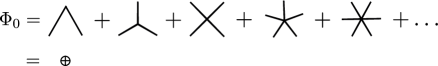
Figure 2: The Rosenfeld functional is the 0-loop approximation of the free-energy. Each intersection diagram corresponds to a completely connected Mayer cluster, contracted into a stack. The sum over all such diagrams is symbolized by a crossed circle.

However, only completely connected Mayer clusters interact in such a way that each particle interacts with each other. Rosenfeld’s functional is therefore the sum over an infinite number of completely connected diagrams that are further contracted into one intersection point.

The arguments, obtained so far, can be summarized in the following way: The exact free-energy functional is not representable by Rosenfeld’s weight densities alone. Instead, the third virial integral (7) is a function of Wertheim’s 2-point densities (6), and it is natural to assume that this result has to be generalized to arbitrary k-point densities. Next, as the Mayer function (2) is itself invariant under coordinate scaling, it is not possible to restrict the functional form by its scaling dimension. From this follows that the three postulates of FMT, including the empirical scaled particle differential equation, have no deeper physical basis. On the other hand, we have also seen that Rosenfeld’s functional approximates and re-summes a certain class of Mayer diagrams contracted to one intersection point, as shown in FIG. 1. This offers an alternative approach to derive the functional and, most importantly, it also opens a path to derive higher order corrections.

The central object of FMT is the sum of contracted intersection diagrams, shown in FIG. 2. Because of its importance, let us introduce the name “stack” for individual parts and “universal stack” for its sum, defined by:

Definition 1

A stack of order $k=\text{ord}(\text{St}_{k})$ is a set of $i=1,\ldots,k$ domains $D_{i}$, intersecting in at least one common point and free to translate and rotate around this center:

$$\text{St}_{k}=\bigcap_{i=1}^{k}D_{i}\;.$$ (10)

The universal stack is the formal sum over all stacks intersecting at the same point

$$\text{USt}=\bigoplus_{i=2}^{\infty}\text{St}_{k}\;.$$ (11)

In the following sections we will prove that the intersection probability of the universal stack $\Phi_{0}$ reproduces Rosenfeld’s functional $\Phi_{\text{R}}$

$$\Phi_{R}=\Phi_{0}\;.$$ (12)

However, this is only the first hint to a more general structure: When completely contracted intersection diagrams correspond to a free-energy functional at low packing fraction, it is natural to assume that diagrams, not completely contracted, provide higher order corrections.

Rosenfeld’s functional is exact for the second virial order. The third virial integral, however, is only an approximation, as shown in FIG. 1. Adding the exact third virial diagram will therefore result in an improved functional, corresponding to three additional intersection centers and the loop constraint (5). In principle, it is possible to add arbitrary intersection diagrams to the functional, systematically derived from the Mayer clusters. As an example consider FIG. 3 where the 4-particle Mayer diagrams are shown together with their corresponding set of intersection diagrams and contractions, ordered by their number of loops $g$ and intersection centers $n$.

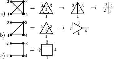
Figure 3: Mayer clusters of the fourth virial order, translated into intersection diagrams and ordered by the tuple $(g,n)$: a) $(3,6)$, $(2,4)$, $(0,1)$, b) $(2,5)$, $(1,3)$, and c) $(1,4)$.

This classification by the tuple $(g,n)$ comes natural as the calculational complexity increases with both. However, they have also a direct physical interpretation.

The loop order $g$ counts the number of constraints, restricting the coordinates of intersection domains:

$$\begin{split}\left.\begin{aligned} \vec{r}_{A_{1}A_{2}}+&\ldots+\vec{r}_{A_{k-1}A_{k}}=0\\ \vec{r}_{B_{1}B_{2}}+&\ldots+\vec{r}_{B_{l-1}B_{l}}\,=0\\ &\ldots\end{aligned}\right\}\quad\text{$g$ loop constrains}\end{split}$$ (13)

for $g$ loops with $k,l,\ldots$ intersection centers. In this way, correlations are generated between particles that otherwise do not interact directly via a potential function. This distinguishes the zero loop order $g=0$, where no such constraints exists, providing a plausible argument why Rosenfeld’s free-energy functional describes only the fluid regime below the first phase transition and predicts a maximum packing fraction at $n_{v}=1$, independent of the particle geometry. The solid phase region, on the other hand, requires long range correlations between particles, such that shifting one particle leads to the displacement of others, as shown in FIG. 4.

Figure 4: The displacement of one particle causes a shift in the position of all neighbors that are in direct and indirect contact, resulting in long range correlations between particles.

These considerations make the number of loops $g$ and intersections $n$ convenient indices to group the diagrams and to define the “loop expansion” of the free-energy excess functional:

$$\Phi^{\text{ex}}=\sum_{g=0}^{\infty}(\sum_{n=1}^{\infty}\Phi_{g,n})=\sum_{g=0}^{\infty}\Phi_{g}\;,$$ (14)

where each element $\Phi_{g,n}$ corresponds itself to an infinite number of intersection diagrams. Examples are shown for $\Phi_{0,1}=\Phi_{0}$ in FIG. 2 and for $\Phi_{1,3}$ in FIG. 5.

Figure 5: The re-summed and regularized third virial integral: Adding additional particles to an existing intersection point does not increase the calculational effort.

It is worth pointing out that some of the contracted 4-particle diagrams of FIG. 3 turn up as corrections of the second and third virial order. Actually, it will be shown in the following sections that the calculational effort does not increase when additional particles are added to an existing intersection point. Any individual intersection diagram can therefore be replaced by a “resummed diagram”, with each intersection point replaced by the universal stack. Resummation is therefore a central aspect of FMT, as it generates the pole structure in the free volume $1-n_{v}$, which is so characteristic for Rosenfeld’s functional.

A natural extension of the current functional is the combination $\Phi_{K}=\Phi_{0,1}+\Phi_{1,3}$, shown in FIG. 6.

Figure 6: Going beyond Rosenfeld’s functional: A first approximation for the 1-loop order contains the re-summed second virial integral and the regularized third virial integral.

However, as parts of $\Phi_{0,1}$ are already included in $\Phi_{1.3}$, it is necessary to “regularize” the loop diagram by excluding the case $|\vec{r}_{AB}|=|\vec{r}_{BC}|=|\vec{r}_{CA}|=0$, shown in FIG. 1, where the distances between the intersection coordinates vanish. All loop diagrams are understood in this way, excluding the case of collapsing loops and thus ensuring that regularized diagrams are uniquely defined.

Apart from the resummation of intersection points, it is also possible to sum up diagrams of identical loop order. One example is displayed in FIG. 7. The analytical structure of the generating function $\Phi_{1}$ can be derived from the virial expansion,

Figure 7: The unregularized free-energy at 1-loop order is the sum over the second virial and all further ring diagrams.

as the ring diagrams are formally identical to Mayer clusters. With the symmetry factor $(k-1)!/2$ for a ring of $k$ particles and the simplifying notation $C^{AB}\omega_{A}\omega_{B}$ for the f-function (2), the 1-loop free-energy yields the formal expression:

$$\begin{split}\Phi_{1}&=\Bigl{<}\sum_{k=1,k\neq 2}^{\infty}\frac{1}{k!}\frac{1}{2}(k-1)!\bigl{(}C^{AB}\omega_{A}\omega_{B}\rho\bigr{)}^{k}\Bigr{>}\\ &=-\frac{1}{2}\Bigl{<}\ln{\bigr{(}1-C^{AB}\omega_{A}\omega_{B}\rho\bigr{)}}\Bigr{>}+\ldots\;,\end{split}$$ (15)

where the angular brackets indicate the integration over the coordinates. The 1-loop free-energy contribution is therefore of a completely different structure than Rosenfeld’s functional, signaling a logarithmic divergence, depending on the particles’ geometry.

Having identified the approximation scheme behind Rosenfeld’s functional, we will now begin with the development of the mathematical framework necessary to derive the intersection probability of the universal stack. In this way, the hypothesis (12) will be proven by direct calculation, which is the basis for the resummation of intersection points and all further constructions that will be considered in following papers.

II.2 Some Relevant Information on Differential Geometry

II.2.1 Intrinsic Geometry

The derivation of the intersection probabilities requires the introduction of some mathematical conventions kobayashi ; guggenheimer ; complex-manifolds-potential and the discussion of physical constraints.

Let $D$ denote an Euclidean, Riemannian manifold of $3$ dimensions, sufficiently differentiable to allow for the calculation of the Euler form. Manifolds of this type include a variety of geometries as convex and concave particles, Klein’s bottle, tori, polyhedrons, cylinders, hollow spheres but also non-compact structures. The mathematical requirements are therefore not very restrictive. However, we also have to take into account the physical constraints. In the formulation of Mayer’s f-functions, the cluster integrals determine the intersection probability between particles. However, the physical particle domain is not only restricted by its surface. Instead one has to determine the region that is inaccessible for other particles. FIG. 8 shows two examples, where the corresponding mathematical intersection probability is zero but not its physical one.

Figure 8: Physical constraints restrict the regions accessible for other particles. Forbidden configurations are: a) linked tori and b) particles inside a cavern (bottle) with pore opening smaller than the particles’ diameter.

FIG. 8a) shows two linked tori. In a fluid of single tori, such a configuration has to be excluded as the particles cannot penetrate each other. The same applies to the system of a particle inside a concave domain, whose opening is smaller than the particle’s smallest diameter, as seen in FIG. 8b). When the geometry of the first does not allow to enter the inner region of the second, it has to be excluded, i.e. counted as part of the domain of the latter particle.

Although physically related, the mathematical nature of these two examples is very different. The case of two tori is related to Euler’s linking number bott-tu ; nash and belongs to the topological class of homotopically non-trivial intersections. Another example is the intersection of hollow spheres as realized by fullerenes. Both cases are related to topological classes that follow by successive variations of Euler forms alvarez-ginsparg . And although they are not required for the current article, they are interesting enough to give a short account further below. The second case FIG. 8b) is more difficult to solve. Here, we have to introduce a fictitious membrane at the opening of the pore, whose surface vector is always antiparallel to the surface vector of the docking particle. Such configurations lead to the vanishing of certain contributions of the intersection probability between particles, as we will show in the next section, and might give new insight into the isotropic-nematic phase transition. Because of these additional complications, we will exclude homotopically non-trivial particles as well as concave geometries. The discussion simplifies further, when boundaries are excluded, leaving us with 3-dimensional convex particles embedded into the flat Euclidean space $\mathbb{R}^{3}$.

The geometry of a physical particle depends on intrinsic and extrinsic properties, i.e. the properties independent and dependent on the embedding. It would be therefore sufficient to consider 2-dimensional surfaces and their embedding into $\mathbb{R}^{3}$. However, at this point it is worthwhile to discuss Cartan’s formulation of differential geometry bruhat ; kobayashi ; guggenheimer for general dimension, as some of the results degenerate for low dimensional spaces.

Let the particle $\Sigma$ be a $n$ dimensional, orientable, differential Riemannian manifold without boundary. Suppose further that the manifold can be covered by a set of open coordinate patches $\Sigma=\cup_{\alpha}U_{\alpha}$, each one isomorphic to $\mathbb{R}^{n}$ and labeled by a local, orthonormal coordinate frame $(p,e_{1}^{(\alpha)},\ldots,e_{n}^{(\alpha)})$ at the point $p\in U_{\alpha}$. The local frames at overlapping regions $U_{\alpha}\cap U_{\beta}$ are related to each other by differentiable coordinate transformations $g_{\alpha\beta}(p):U_{\alpha}\cap U_{\beta}\to\text{SO}(n)$. The matrix valued transition functions $g_{\alpha\beta}$ are invertible $g_{\alpha\beta}^{-1}=g_{\beta\alpha}$ and fulfill the cyclic condition $g_{\alpha\beta}g_{\beta\gamma}g_{\gamma\alpha}=1$ at triple intersections $U_{\alpha}\cap U_{\beta}\cap U_{\gamma}$. These preliminaries define the tangential bundle $T\Sigma$ with the local section $(p,e_{1},\ldots,e_{n})\in\Gamma(T\Sigma)$ and the cotangential bundle $T^{*}\Sigma$ as its dual space, related to $T\Sigma$ by the metric of $\mathbb{R}^{n}$

$$e_{i}\cdot e_{j}=\eta_{ij}$$ (16)

and its differential structure. The vielbein $\theta_{i}$ and connection forms $\omega_{ij}$ are defined by

$$dp=e_{i}\theta_{i}\;,\quad de_{i}=\omega_{ij}e_{j}\quad\text{for}\quad p\in\Sigma$$ (17)

and transform under the coordinate change $e_{i}^{\prime}=g_{ij}e_{j}$ as

$$\theta_{i}^{\prime}=g_{ij}\theta_{j}\;,\quad\omega_{ij}^{\prime}=g_{ki}^{-1}\omega_{kl}g_{lj}+g_{ki}^{-1}dg_{kj}\;,$$ (18)

where summation over paired indices is understood. The connection is therefore not a tensor and can be locally replaced by a trivial gauge.

The vanishing of the second exterior derivative of (17) defines the torsion and the curvature form

$$T_{i}=d\theta_{i}-\omega_{ij}\wedge\theta_{j}\;,\quad\Omega_{ij}=d\omega_{ij}-\omega_{ik}\wedge\omega_{kj}\;,$$ (19)

which transform as a first and second rank tensor

$$T_{i}^{\prime}=g_{ij}T_{j}\;,\quad\Omega^{\prime}_{ij}=g_{ki}^{-1}\Omega_{kl}g_{lj}\;.$$ (20)

The constraint $T_{i}=0$ of a Riemannian manifold is therefore independent of the coordinate system and introduces a global relationship between the vielbein and the connection forms.

Torsion and curvature carry local information about the geometry of a manifold, always restricted to single coordinate patches $U_{\alpha}$ and depending on the chosen coordinate system. Globally defined forms, on the other hand, are necessarily invariant under coordinate transformations. An important class of such functions was introduced by Chern chern-curv-integra ; complex-manifolds-potential in extending the notion of class functions $f(g^{-1}xg)=f(x)$ from group theory. From (19) follows that the curvature form transforms under the adjoint representation of $\text{SO}(n)$. Natural choices are therefore the determinant and the trace of a polynomial in $\Omega$, whose differential form is of the same order as the volume form of $\Sigma$ or any submanifold thereof. Chern defined the Euler form or Euler class

$$\text{Pf}(\Omega)=\frac{1}{n!}\epsilon^{i_{1}\ldots i_{n}}\Omega_{i_{1}i_{2}}\wedge\ldots\Omega_{i_{n-1}i_{n}}$$ (21)

for even dimensional manifolds $n=2k$ and its integral as the Euler characteristic

$$\chi(\Sigma)=\frac{(-1)^{k}(2k)!}{(4\pi)^{k}k!}\int_{\Sigma}\text{Pf}(\Omega)\;,$$ (22)

with the normalization chosen such that its result is whole-numbered for the sphere $\chi(S^{2})=2$ and the $g$-holed torus $\chi(T^{2}_{g})=2-2g$. The integral is a topological invariant and central for many areas of mathematics and physics nash . It is therefore not surprising to discover that the Euler form also enters the discussion of hard particle physics as the intersection probability of particle stacks.

The Euler class is the highest possible form for even dimensional manifolds from which derives a series of invariant differential forms by successive variation $\delta\omega=g^{-1}dg$. The resulting Chern-Simons classes complex-manifolds-potential ; alvarez-ginsparg determine the failure of the form to be invariant under the coordinate transformations (18). As an example consider the case of $n=2$ dimensional manifolds with the transition function $g=\exp{(i\lambda)}\in\text{U}(1)$. The curvature reduces to the exterior derivative $\Omega=d\omega$ and its variation $\delta\omega=id\lambda$ to a $i\mathbb{R}$ valued function:

$$\delta\int_{\Sigma}\epsilon_{ij}\Omega_{ij}=\delta\int_{\partial\Sigma}\epsilon_{ij}\omega_{ij}=\int_{\partial\Sigma}id\lambda=\int_{\partial\partial\Sigma}i\lambda\;.$$ (23)

When the first integrant is rewritten by the Gaussian curvature $K$, the second by the geodesic curvature $\kappa_{g}$ and the last integrant by the interior angles, we obtain from (22) the Gauss-Bonnet equation for the 2-dimensional surface $\Sigma$

$$2\pi\chi(\Sigma)=\int_{\Sigma}Kd\sigma+\int_{\partial\Sigma}\kappa_{g}ds+\sum_{i}(\pi-\alpha_{i})$$ (24)

with non-contractible curves along $\partial\Sigma$ and additional vertices at the singular points. To get a better understanding of the origin of these additional contributions, remember that the Euler form counts the angular change of the normal vector, while moving over the surface of the embedded manifold. For smooth, Riemannian surfaces this is always $4\pi$, but boundaries and singular points contribute additional angular changes and generate the Chern-Simons terms.

It can be shown complex-manifolds-potential ; alvarez-ginsparg that the two equations $\Omega=d\omega$, $\delta\omega=id\lambda$ generalize for the Euler form $Q_{2k}^{0}:=\text{Pf}(\Omega)$ for arbitrary even dimension to a sequence of characteristic classes

$$\delta Q_{2k}^{0}=dQ_{2k-1}^{0}\;,\quad\delta Q_{2k-m}^{m-1}=dQ_{2k-m-1}^{m}$$ (25)

for $m=1,\ldots,2k$. Each variation now produces a new characteristic form of one order less than its predecessor. And in the same way as the geodesic curvature is an invariant form for the 1-dimensional curve $\partial\Sigma$, it is natural to apply the odd differential forms of $Q_{2k-m-1}^{m}$ to odd dimensional manifolds of non-trivial homotopy group. Euler’s linking number and the intersection number of hollow spheres are special cases of these forms. In the notation of alvarez-ginsparg , they correspond to $Q^{1}_{2}$ and $Q^{2}_{3}$ and derive from the Euler class of a 4 and 6 dimensional manifold. However, for convex geometries, which we will consider in the following, it is not necessary to take these classes into account.

Apart from the geometric interpretation of a Riemannian manifold, there is also the relation to Lie groups, whose vielbein and connection forms constitute the basis of a Lie algebra kobayashi ; helgason ; santalo-book represented by the matrix

$$\sigma_{A}=\begin{pmatrix}\omega_{ij}&\theta_{i}\\ -\theta_{j}&0\end{pmatrix}\in\text{iso}(n)\;,$$ (26)

whose elements satisfy the Maurer-Cartan equations

$$\begin{split}d\sigma^{A}&=\omega^{A}_{\;B}\wedge\sigma^{B}=\frac{1}{2}C^{A}_{BC}\sigma^{C}\wedge\sigma^{B}\\ d^{2}\sigma^{A}&=0=\frac{1}{2}C^{A}_{BC}C^{C}_{DE}\sigma^{B}\wedge\sigma^{D}\wedge\sigma^{E}\;.\end{split}$$ (27)

They are related by the inner derivation $i_{B}\sigma_{A}=\sigma_{A}(X_{B})=\eta_{AB}$ to the more commonly used commutation relation $[X_{A},X_{B}]=C_{AB}^{C}X_{C}$ and Jacobi identity. The corresponding Lie group is the Euclidean or isometric group that locally splits into the semi-direct product $\text{ISO}(n)=\text{SO}(n)\ltimes E_{n}$ of rotations and translations. Its Lie algebra elements $\omega_{ij}$ and $\theta_{i}$ transform under the mapping (18) and span a $n(n+1)/2$ dimensional space consisting of the $n(n-1)/2$ connection and $n$ vielbein forms.

The integral over all rotations and translations is therefore related to Haar’s measure of the isometric group

$$\begin{split}&\wedge_{i<j=1}^{n}\omega_{ij}\wedge_{i=1}^{n}\theta_{i}\\ &=\wedge_{i=1}^{n-1}\omega_{in}\wedge_{i=1}^{n-2}\omega_{in-1}\wedge\ldots\wedge\omega_{12}\wedge d\text{vol}(E_{n})\\ &=dS^{n-1}\wedge dS^{n-2}\wedge\ldots\wedge dS^{1}\wedge d\text{vol}(E_{n})\\ &=d\text{vol}(\text{SO}(n))\wedge d\text{vol}(E_{n})\;,\end{split}$$ (28)

where we made use of the coset representation:

$$\text{SO}(k)/\text{SO}(k-1)=S^{k-1}\;.$$ (29)

Evaluating the integral yields then a product of volumes of spheres, with values:

$$O_{k}=\text{vol}(S^{k})=\frac{2\pi^{\frac{k+1}{2}}}{\Gamma(\frac{k+1}{2})}\;,$$ (30)

whose first elements are $O_{1}=2\pi$, $O_{2}=4\pi$, ….

II.2.2 Extrinsic Geometry

Up to now, we have only considered the intrinsic properties of the particles’ geometry. However, the movement in a background space requires the choice of a suitable embedding. For physical reasons it is natural to consider the flat Euclidean space and to imbed the $k$ dimensional particle, e.g., into the first coordinate directions of the local frame $(e_{1},\ldots,e_{k},e_{k+1},\ldots e_{n})$ with the corresponding nontrivial coordinate transformations $\text{ISO}(n)/(\text{ISO}(k)\times\text{ISO}(n-k))$. To avoid the additional problems that occur when discussing this complicated coset structure, we will restrict the dimension of the embedding to $k=n-1$. The group $\text{ISO}(1)$ consists then only of the translation in one direction and can be explicitly separated in the following equations.

This choice is the simplest possible embedding and at the same time also the physically most relevant one. The manifold $D\hookrightarrow\mathbb{R}^{n}$ is now a $n$-dimensional domain in $\mathbb{R}^{n}$ and bounded by its surface $\partial D$. Following the outline of chern-1 , we choose the outward normal direction of the surface to point along $e_{n}$, such that the tangential directions of $\partial D$ correspond to the first $n-1$ elements of the local frame $(e_{1},\ldots,e_{n-1},e_{n})$ of $\mathbb{R}^{n}$. The corresponding directions are differenced by the index convention:

$$i,j=1,\ldots n\quad\text{and}\quad\alpha,\beta=1,\ldots,n-1\;.$$ (31)

The associated Pfaff system kobayashi ; bruhat of the integrable submanifold is then defined by the constraint

$$\theta_{n}=0\quad\text{on}\quad\partial D\;.$$ (32)

Applied to the vanishing torsion of the Riemannian manifold

$$0=d\theta_{n}=\omega_{n\alpha}\wedge\theta_{\alpha}=h_{\alpha\beta}\theta_{\beta}\wedge\theta_{\alpha}=\kappa_{\alpha}\nu_{\alpha}\wedge\nu_{\alpha}\;,$$ (33)

it allows an algebraical solution of the equation by the symmetric matrix $h_{\alpha\beta}$ and to define the principal curvatures $\kappa_{\alpha}$ and principal vectors $\nu_{\alpha}$ as its eigenvalues and orthonormal eigenvectors. In the form, $de_{n}=\kappa_{\alpha}\nu_{\alpha}e_{\alpha}$, it is also known as Rodrigues formula.

Splitting the $n$-dimensional curvature $\Omega^{(n)}$ into normal and tangential directions

$$\begin{split}\Omega^{(n)}_{n\alpha}&=d\omega_{n\alpha}-\omega_{\alpha\beta}\wedge\omega_{\beta n}\\ &=D^{(n-1)}\omega_{n\alpha}\\ \Omega^{(n)}_{\alpha\beta}&=d\omega_{\alpha\beta}-\omega_{\alpha\gamma}\wedge\omega_{\gamma\beta}-\omega_{\alpha n}\wedge\omega_{n\beta}\\ &=\Omega_{\alpha\beta}^{(n-1)}-\omega_{\alpha n}\wedge\omega_{n\beta}\end{split}$$ (34)

yields the Gauss and Gauss-Codazzi equations kobayashi , further reducing to

$$\Omega_{\alpha\beta}^{(n-1)}=\omega_{\alpha n}\wedge\omega_{n\alpha}\quad\text{and}\quad D^{(n-1)}\omega_{n\alpha}=0$$ (35)

in the case of flat embedding. The first equation relates the intrinsic curvature of the particle to the normal connection forms of the embedding. Whereas the vanishing of $\omega_{n\alpha}$ under the $n-1$ dimensional covariant derivative ensures the decoupling of the normal coordinate transformations from the tangential ones; the forms $\omega_{n\alpha}$ are therefore horizontal kobayashi , without the need of introducing equivariant differential forms greub .

In the definition of the embedding we have assumed that the normal vector $e_{n}$ points outward from the compact particle surface. This corresponds to a special gauge choice in the $\text{O}(n)$ coordinate transformations of $\mathbb{R}^{n}$ and restricts the group to $\text{SO}(n)$. But this local gauge does not extend globally, where both orientations $\mathbb{Z}_{2}\cong\text{O}(n)/\text{SO}(n)$ have to be taken into account. The Euler characteristic, derived by the intrinsic curvature (19) and by Gauss’s equation (35), will correspondingly differ by a factor of two

$$\chi(\partial D)=2\chi(D\hookrightarrow\mathbb{R}^{n})\;.$$ (36)

The kinematic measure (28) of an embedded particle of odd dimension $n=2k+1$ can now be calculated by combining (21, 22, 35, 36) and observing that the normalization of the Euler characteristic is proportional to $O_{2k}=2(4\pi)^{k}k!/(2k)!$, as follows from (30)

$$\int\wedge_{i<j=1}^{2k+1}\omega_{ij}\wedge_{i=1}^{2k+1}\theta_{i}$$

$$=\int\text{Pf}(\Omega)\wedge d\text{vol}(\text{SO}(2k))\wedge d\text{vol}(E_{2k+1})$$ (37)

$$=\chi(\partial D)\,\text{vol}(\text{SO}(2k+1))\,\text{vol}(E_{2k+1})\;.$$

For a 3-dimensional manifold in $\mathbb{R}^{3}$, the corresponding integral reduces to

$$\int \omega_{12}\omega_{13}\omega_{23}\theta_{1}\theta_{2}\theta_{3}=\int\kappa_{1}\kappa_{2}\nu_{1}\nu_{2}\cdot\int\omega_{12}\,d\text{vol}(\mathbb{R}^{3})$$

$$=\int K(\partial D)dS_{A}\cdot 2\pi\,V$$

$$=8\pi^{2}V\int\frac{1}{4\pi}K(\partial D)\delta(\vec{n}\vec{r}_{A})d^{3}r_{A}$$ (38)

$$=8\pi^{2}\,V\,\chi(\partial D)$$

with the volumes of $\text{vol}(\mathbb{R}^{3})=V$ and $\text{vol}(\text{SO}(3))=8\pi^{2}$.

Note that the kinematic measure of a Riemannian manifold would vanish for dimensional reasons, as the vielbein and connection forms are not independent. It is therefore necessary first to interpret the integrant as the Haar’s measure and only afterwards to incorporate the geometric constraints.

This equation is of course closely related to Chern’s original derivation of the Euler class chern-curv-integra . Here however, the difference lies in the relation between geometry and isometric group, which focuses on the alternative interpretation as the kinematic measure of a particle, moving in a flat background. For two intersecting particles it thus determines the intersection probability, averaged over all rotations and translations. It is therefore identical to the second virial integral and explains the appearance of the Gauss-Bonnet equation (24) in the calculations of Isihara and Kihara kihara-1 , Rosenfeld rosenfeld2 , and Wertheim wertheim-1 .

II.3 The One, Two, and Three Particle Intersections

II.3.1 Comments on Integral Geometry

The generalization of (II.2.2) to two and more intersecting particles leads us into the field of integral geometry, whose differential geometric formulation goes back to Minkowski minkowski , Weyl weyl-tube , Blaschke blaschke , Santalo santalo-book , and Chern chern-1 ; chern-2 ; chern-3 , who observed that the invariant forms of integral geometry can be traced back to the Euler class (II.2.2). One intriguing result is the fundamental kinematic equation santalo-book

$$\begin{split}\frac{V_{n}}{\gamma_{n}}\int\limits_{\text{ISO}(n)}\chi(D_{1}\cap gD_{2})dg&=\sum_{k=0}^{n}\binom{n}{k}M_{k}(D_{1})M_{n-k}(D_{2})\\ \gamma_{n}=\text{vol}(\text{SO}(n))\;&,\quad V_{n}=\frac{1}{n}O_{n-1}\end{split}$$ (39)

and the observation that the coupled geometry of two intersecting manifolds reduces to a simple pairwise product of Minkowski measures or integrals of mean curvature $M_{k}$. For $n=3$ it reproduces the equation of Isihara and Kihara of the second virial coefficient. Actually, they used for their calculation an early result of Minkowski minkowski . In fact, it was the starting point for our current investigation and offers a direct, albeit less general, approach of deriving the intersecting probability, which is why we have added their calculation in a somewhat clarified form in appendix A.

There are several ways to derive the fundamental kinematic equation (39). Probably the simplest one uses the expansion of the Steiner polynomial santalo-book , another one Blaschke’s cut and paste construction blaschke of subspaces. The most fundamental, although more elaborate approach is Chern’s explicit derivation chern-1 of the Euler class from the kinematic measure (II.2.2). Its advantage is the explicit local formulation in connection forms that will be important for its decoupling into Rosenfeld’s weight functions. This ansatz is therefore the natural starting point for relating Rosenfeld’s approach to integral geometry.

The generalization of (II.2.2) to a particle stack $\text{St}_{k+1}$ is easily achieved but requires some normalization to get a well defined result. First, we have to fix the position and orientation of one particle in $\text{St}_{k+1}$ to remove the volume dependence on the embedding space $V=\text{vol}(\mathbb{R}^{3})$, generated by moving the stack in the background manifold. Furthermore, it is useful to define the kinematic measures of the particle domain $D$ and its surface $\Sigma$

$$\begin{split}dD&=\omega_{12}\omega_{13}\omega_{23}\wedge\theta_{1}\theta_{2}\theta_{3}\\ d\Sigma&=\omega_{12}\wedge\theta_{1}\theta_{2}\end{split}$$ (40)

analogously to (3). The kinematic measure of (II.2.2) or (II.2.2) generalizes then to the integral average of $k+1$ particles

$$\begin{split}\frac{1}{8\pi^{2}}&\frac{1}{V}\int_{St_{k+1}}\,dD_{1}\wedge\ldots\wedge dD_{k+1}\\ &=\frac{1}{4\pi}\int_{\text{St}_{k+1}}K(\partial\text{St}_{k+1})\,\delta(\vec{n}\vec{r}_{A})\,d^{3}r_{A}\\ &\qquad\qquad\qquad\times d\gamma_{2}\wedge\ldots\wedge d\gamma_{k+1}\;,\end{split}$$ (41)

with the Gaussian curvature $K$ integrated over the domain $A=\text{St}_{k+1}$ at fixed kinematic measure $\gamma$, as defined in (3), and integrated over the center of gravity, represented by $\gamma_{1}$.

The boundary of the stack $\partial\text{St}_{k+1}$ can be determined by the algebraic relations of the homology operator bott-tu . As an example, consider two intersecting manifolds that itself have no boundary $\partial^{2}D=0$. The application of $\partial$ to the second order stack

$$\partial(D_{1}\cap D_{2})=\partial D_{1}\cap D_{2}+D_{1}\cap\partial D_{2}+\partial D_{1}\cap\partial D_{2}\;.$$ (42)

is thus a sum of intersections, wherein each successive application of $\partial$ reduces the dimension by one. This restricts the possible number of boundary operations to the dimension of the embedding space by the constraint $\partial^{4}X=0$ for any 3-dimensional manifold $X$. The infinite number of virial contributions, shown in FIG. 2, reduces therefore to the derivation of three Euler forms, corresponding to one, two, and three particles.

The calculation of (41) can be further simplified by including the physical constraint of indistinguishable particles. To obtain the correct combinatorial pre-factors, let us define the formal sum

$$\hat{n}=\sum_{i=1}^{M}D_{i}\,\rho_{i}$$ (43)

of 1-particle densities and domains. It is the homologous operator of Rosenfeld’s weight densities and parallels the notion of a divisor in algebraic geometry. The representation of the free-energy functional in $\hat{n}$ reduces the problem of determining the boundary of the stack of $k+1$ different particles $\partial\text{St}_{k+1}$ to the corresponding analysis of a stack of $k+1$ identical manifolds, whose boundary reduces to a sum of three terms

$$\begin{split}\partial\text{St}_{k+1}&=(k+1)\,\Sigma\cap\text{St}_{k}+(k+1)k\,\Sigma\cap\Sigma\cap\text{St}_{k-1}\\ &+(k+1)k(k-1)\,\Sigma\cap\Sigma\cap\Sigma\cap\text{St}_{k-2}\end{split}$$ (44)

in the shorthand notation $\Sigma=\partial D$. Using the linearity of the Euler form and its vanishing for odd dimensional manifolds, it translates to the corresponding Gaussian curvature

$$\begin{split}K(\partial\text{St}_{k+1})&=(k+1)\,K(\Sigma)+(k+1)k\,K(\Sigma\cap\Sigma)\\ &+(k+1)k(k-1)\,K(\Sigma\cap\Sigma\cap\Sigma)\end{split}$$ (45)

that will be derived in the following. The first two terms are known from Chern chern-1 , who obtained the result for two intersecting manifolds of arbitrary dimension. An independent approach was used by Wertheim wertheim-1 . However, the three-particle intersection is new and will be presented parallel to the summary of the previous two cases. The corresponding generalization of Chern’s approach to an arbitrary number of particles and dimensions has been developed in korden and will now be applied to three dimensions.

II.3.2 The One Particle Euler Form

Let us begin with the simplest case $K(\Sigma)$ of one particle, moving in a background of $k$ domains. Following the derivation of (II.2.2) the product of the connection forms can be rewritten in the principal basis $\omega_{13}\wedge\omega_{23}=\kappa_{1}\kappa_{2}\nu_{1}\wedge\nu_{2}$, reducing the kinematic measure of $\Sigma$

$$\begin{split}&\frac{1}{8\pi^{2}}\frac{1}{V}\int_{\Gamma(D_{1})}dD_{1}=\frac{1}{8\pi^{2}}\frac{1}{V}\int_{\Gamma(D_{1})}\omega_{13}\omega_{23}\omega_{12}\theta_{1}\theta_{2}\theta_{3}\\ &=\frac{1}{4\pi}\int_{A=D_{1}}\kappa_{G}\,\delta(\vec{n}\vec{r}_{A})\,d^{3}r_{A}\end{split}$$ (46)

with the Gaussian curvature $\kappa_{G}$ and a factor of $2\pi$ from the integral over $\omega_{12}$. The first part of the integral (44) for a stack can now be written as

$$\frac{1}{4\pi}\int_{\begin{subarray}{c}\Gamma(D_{2}\times\ldots\times D_{k+1})\\ \times\text{St}_{k+1}\end{subarray}}K(\Sigma_{1},\vec{r}_{A})\,\delta(\vec{n}\vec{r}_{A})\,d^{3}r_{A}\,dD_{2}\ldots dD_{k+1}$$

$$=\int\frac{1}{4\pi}\kappa_{G}(\partial D_{1},\vec{r}_{A})\,\delta(\vec{n}\vec{r}_{A})\,\Theta(D_{2},\vec{r}_{A})\ldots\Theta(D_{k+1},\vec{r}_{A})$$

$$\qquad\qquad\qquad\times d^{3}r_{A}\,d\gamma_{2}\ldots d\gamma_{k+1}$$

$$=\int\omega_{\chi}^{(1)}\omega_{v}^{(2)}\ldots\omega_{v}^{(k+1)}d^{3}r_{A}\,d\gamma_{2}\ldots d\gamma_{k+1}$$ (47)

in the weight functions

$$\omega_{\chi}^{(i)}=\frac{1}{4\pi}\kappa_{G}\,\delta(\partial D_{i})\;,\quad\omega_{v}^{(i)}=\Theta(D_{i})\;,$$ (48)

where the integration domain has been formally extended to the complete embedding space $V$ by the Dirac- and Heaviside-function $\delta$ and $\Theta$, with $\delta(\partial D_{i})$ understood as restricting the volume integration to the surface $\delta(\vec{n}\vec{r}_{A})$ at the intersection point $\vec{r}_{A}\in\text{St}_{k}$.

II.3.3 The Two Particle Euler Form

Some more efforts requires the derivation of the second Euler form $K(\Sigma_{1}\cap\Sigma_{2})$ that determines the angular change between the two normal vectors at the 1-dimensional intersection submanifold. It parallels the geodesic curvature $\kappa_{g}$ of the Gauss-Bonnet formula (24) and can be seen as the real space generalization of the Chern-Simons class. Its derivation begins with the construction of a proper coordinate system at the intersection space. Let us introduce the bases $\Sigma_{1}:(e_{1},e_{2}^{(1)},e_{3}^{(1)})$ and $\Sigma_{2}:(e_{1},e_{2}^{(2)},e_{3}^{(2)})$ with the common direction $\Sigma_{1}\cap\Sigma_{2}:e_{1}$ along the 1-dimensional submanifold and the intersection angle

$$\cos{(\phi_{12})}=(e_{3}^{(1)}e_{3}^{(2)})\quad\text{for}\quad 0\leq\phi_{12}<2\pi\;.$$ (49)

Following korden , we define the intersection determinant

$$M_{k}=\det{(e_{3}^{(i)}e_{3}^{(j)})}|_{i,j=1}^{k}$$ (50)

for $k$ intersecting surfaces. The first two cases are:

$$\begin{split}M_{2}&=1-c_{12}^{2}=s_{12}^{2}\\ M_{3}&=1-c_{12}^{2}-c_{13}^{2}-c_{23}^{2}+2c_{12}c_{13}c_{23}\;,\end{split}$$ (51)

where we used the shorthand notation:

$$\begin{split}s_{ij}:=\sin{(\phi_{ij})}\;&,\quad c_{ij}:=\cos{(\phi_{ij})}\\ s(\gamma):=\sin{(\gamma)}\;&,\quad c(\gamma):=\cos{(\gamma)}\;.\end{split}$$ (52)

The local frame of the intersection manifold in $\mathbb{R}^{3}$ is spanned by the vector field $e_{1},e_{3}^{(1)},e_{3}^{(2)}$ for $\phi_{12}\neq 0$, from which one obtains an orthonormal basis by the Gram-Schmidt process

$$v_{3} =e_{3}^{(1)}$$

$$v_{2} =\frac{1}{s_{12}}\bigl{(}e_{3}^{(2)}-c_{12}\,e_{3}^{(1)}\bigr{)}$$ (53)

$$v_{1} =e_{1}\;.$$

As explained before, the Euler characteristic counts the angular change of the normal vector, while moving from $e_{3}^{(1)}$ to $e_{3}^{(2)}$. To interpolate between those two vectors, we introduce a $\text{SO}(2)$ rotation in the range $0\leq\gamma\leq\phi_{12}$

$$\begin{split}\eta_{3}&=c(\gamma)v_{3}+s(\gamma)v_{2}\\ \eta_{2}&=-s(\gamma)v_{3}+c(\gamma)v_{2}\\ \eta_{1}&=e_{1}\;.\end{split}$$ (54)

One of the two equivalent vectors, $\eta_{3}$ or $\eta_{2}$, is now the new outward pointing normal direction. Let us chose $\eta_{3}$ and derive the corresponding Euler density for the intersection $\Sigma_{1}\cap\Sigma_{2}$:

$$\begin{split}\eta_{1}d\eta_{3}&\wedge\eta_{2}d\eta_{3}\\ &=\frac{1}{s_{12}}\left[s(\phi_{12}-\gamma)\omega_{13}^{(1)}+s(\gamma)\omega_{13}^{(2)}\right]\wedge d\gamma\;,\end{split}$$ (55)

with the definition $\omega_{13}^{(i)}=e_{1}de_{3}^{(i)}$ of the new connection forms for the particles $i=1,2$. Integrating over $\gamma$

$$\begin{split}\int\eta_{1}d\eta_{3}\wedge\eta_{2}d\eta_{3}&=\frac{1-c_{12}}{s_{12}}[\omega_{13}^{(1)}+\omega_{13}^{(2)}]\\ &=K(\Sigma_{1}\cap\Sigma_{2})d(\Sigma_{1}\cap\Sigma_{2})\end{split}$$ (56)

yields the differential Euler form. Observe, that the angular dependent factor $(1-c_{12})/s_{12}$ remains finite even in the limit of anti-parallel vectors $\phi_{12}\to\pi$ when the remaining kinematic measure is included, which will be derived below.

At the intersection $\Sigma_{1}\cap\Sigma_{2}$, a $\text{SO}(2)$ transformation (18) relates the vector frames of the two particles

$$\begin{split}e_{3}^{(2)}&=c_{12}e_{3}^{(1)}+s_{12}e_{2}^{(2)}\\ e_{2}^{(2)}&=-s_{12}e_{3}^{(1)}+c_{12}e_{2}^{(2)}\\ e_{1}^{(2)}&=e_{1}^{(1)}\end{split}$$ (57)

and the boundary condition $\theta_{3}^{(i)}|_{\partial\Sigma_{i}}=0$ their corresponding Pfaffian systems (32). The transformed differential forms

$$\begin{split}\theta_{3}^{(2)}&=c_{12}\theta_{3}^{(1)}+s_{12}\theta_{2}^{(1)}\\ \omega_{13}^{(2)}&=c_{12}\omega_{13}^{(1)}+s_{12}\omega_{12}^{(1)}\\ \omega_{23}^{(2)}&=\omega_{23}^{(1)}+d\phi_{12}\end{split}$$ (58)

are therefore understood modulo $\theta_{3}^{(1)},\omega_{\alpha 3}^{(1)}$. With these relations, the reduced kinematic measure of $\Sigma_{1}\cap\Sigma_{2}$ can be derived, with the first particle fixed in the embedding space and the second one free to move:

$$d( \Sigma_{1}\cap\Sigma_{2})\wedge dD_{2}$$

$$=\theta_{1}^{(1)}\wedge\theta_{1}^{(2)}\theta_{2}^{(2)}\theta_{3}^{(2)}\omega_{12}^{(2)}\omega_{13}^{(2)}\omega_{23}^{(2)}$$

$$=(s_{12})^{2}\;\theta_{1}^{(1)}\theta_{2}^{(1)}\omega_{12}^{(1)}\wedge\theta_{1}^{(2)}\theta_{2}^{(2)}\omega_{12}^{(2)}\wedge d\phi_{12}$$ (59)

$$=(s_{12})^{2}\;d\Sigma_{1}\wedge d\Sigma_{2}\wedge d\phi_{12}\;,$$

with the kinematic measure of the surface defined in (40). The decoupling of the Euler form (56) and the kinematic measure (II.3.3) for two intersecting particles is a central property of integral geometry santalo-book and follows from the $\text{ISO}(3)$ invariance.

Next, we transform $(e_{1}^{(i)},e_{2}^{(i)},e_{3}^{(i)})$ into the orthonormal coordinate system of the principal frame $(\vec{\nu}_{1}^{(i)},\vec{\nu}_{2}^{(i)},\vec{n}^{(i)})$, changing the notation for the normal direction $\vec{n}=e_{3}$ to be consistent with Rosenfeld’s and Wertheim’s convention. The 3-dimensional cross product of the normal vectors

$$e_{1}=v_{1}=v_{2}\wedge v_{3}=\frac{1}{s_{12}}\;\vec{n}^{(2)}\times\vec{n}^{(1)}\;$$ (60)

points now into the tangential direction of the intersection. Combining the Euler form and the kinematic measure, we obtain the intersection probability between two particles:

$$\begin{split}&\frac{1}{8\pi^{2}}\frac{1}{V}\int_{\Gamma(D_{1}\times D_{2})}dD_{1}\wedge dD_{2}\\ &=\frac{1}{4\pi}\int_{\Gamma(D_{2})}\int_{\Sigma_{1}\cap\Sigma_{2}}K(\Sigma_{1}\cap\Sigma_{2})d(\Sigma_{1}\cap\Sigma_{2})dD_{2}\\ &=\frac{1}{4\pi}\int_{\Gamma(D_{2})}\int_{\Sigma_{1}\cap\Sigma_{2}}\frac{1-c_{12}}{s_{12}}[\omega_{13}^{(1)}+\omega_{13}^{(2)}]\;dD_{2}\end{split}$$ (61)

integrated over the intersection volume $A=D_{1}\cap D_{2}$ and the kinematic measure with $\phi_{12}\in\Gamma(D_{2})$.

The transformation of the connection forms from the old reference system to the principal frame was done by Chern chern-1 . However, Wertheim’s tensorial representation wertheim-1 (see also rosenfeld2 ; rosenfeld-gauss2 ; mecke-fmt ; goos-mecke ) has the advantage to be more closely related to Rosenfeld’s definition of weight functions. In order to keep the discussion self-contained, we have included Wertheim’s derivation in appendix B and present here only the result.

Using the diagonal form of the Euclidean metric $\mathbb{I}$ and the curvature tensor $\mathbb{K}$

$$\begin{split}\mathbb{I}&=\vec{\nu}_{1}\otimes\vec{\nu}_{1}+\vec{\nu}_{2}\otimes\vec{\nu}_{2}+\vec{n}\otimes\vec{n}\\ \mathbb{K}&=\kappa_{1}\,\vec{\nu}_{1}\otimes\vec{\nu}_{1}+\kappa_{2}\,\vec{\nu}_{2}\otimes\vec{\nu}_{2}\;,\end{split}$$ (62)

Rodrigues formula (33) yields the form:

$$e_{1}de_{3}=e_{1}\mathbb{K}e_{1}\,ds=e_{1}[\bar{\kappa}(\mathbb{I}-\vec{n}\otimes\vec{n})+\Delta]e_{1}\,ds$$ (63)

with the mean and tangential curvature

$$\bar{\kappa}=\frac{1}{2}(\kappa_{1}+\kappa_{2})\;,\quad\Delta=\frac{1}{2}(\kappa_{1}-\kappa_{2})(\nu_{1}\otimes\nu_{1}-\nu_{2}\otimes\nu_{2})\;.$$ (64)

With this change of notations and appendix B, we finally obtain Wertheim’s representation of the kinematic measure

$$\frac{1}{4\pi}\int_{\Gamma(D_{2})}\int_{\Sigma_{1}\cap\Sigma_{2}}K(\Sigma_{1}\cap\Sigma_{2})d(\Sigma_{1}\cap\Sigma_{2})dD_{2}$$

$$=\frac{1}{4\pi}\int_{\Gamma(D_{2})}\int_{A=D_{1}\cap D_{2}}\Bigl{[}(\mathbb{I}-\vec{n}^{(1)}\otimes\vec{n}^{(2)})(\bar{\kappa}^{(1)}+\bar{\kappa}^{(2)})\Bigr{.}$$ (65)

$$\quad\Bigl{.}-\frac{\vec{n}^{(1)}\Delta^{(2)}\vec{n}^{(1)}+\vec{n}^{(2)}\Delta^{(1)}\vec{n}^{(2)}}{1+\vec{n}^{(1)}\vec{n}^{(2)}}\Bigr{]}$$

$$\quad\times\delta(\vec{n}^{(2)}\vec{r}_{A})\delta(\vec{n}^{(1)}\vec{r}_{A})\,d^{3}r_{A}\,dD_{2}$$

integrated over $\vec{r}_{A}\in D_{1}\cap D_{2}$ and $\Gamma(D_{2})$.

Now it is a simple task to expand the denominator in the geometric series

$$\frac{1}{1+\vec{n}^{(1)}\vec{n}^{(2)}}=1-\vec{n}^{(1)}\vec{n}^{(2))}+(\vec{n}^{(1)})^{\otimes 2}(\vec{n}^{(2))})^{\otimes 2}\pm\ldots$$ (66)

of tensor products and to rewrite the integral in the weight functions

$$\begin{split}&\frac{1}{4\pi}\int_{\begin{subarray}{c}\Gamma(D_{2}\times\ldots\times D_{k+1})\\ \times\Sigma_{1}\cap\Sigma_{2}\end{subarray}}K(\Sigma_{1}\cap\Sigma_{2})d(\Sigma_{1}\cap\Sigma_{2})dD_{2}\ldots dD_{k+1}\\ &=\int_{\begin{subarray}{c}\Gamma(D_{2}\times\ldots\times D_{k+1})\\ \times\text{St}_{k+1}\end{subarray}}\Bigl{[}\omega_{\kappa 0}^{(1)}\omega_{\sigma 0}^{(2)}-\omega_{\kappa 1}^{(1)}\omega_{\sigma 1}^{(2)}-\sum_{L=0}^{\infty}\omega_{\Delta L+2}^{(1)}\omega_{\sigma L}^{(2)}\Bigr{.}\\ &\qquad\Bigl{.}+(1\leftrightarrow 2)\;\Bigr{]}\,\omega_{v}^{(3)}\ldots\omega_{v}^{(k+1)}\;d^{3}r_{A}\,d\gamma_{2}\ldots d\gamma_{k+1}\end{split}$$ (67)

with the extended basis set of Rosenfeld’s weight functions:

$$\begin{split}\omega_{\chi}(D)&=\frac{1}{4\pi}\kappa_{G}\,\delta(\partial D)\\ \omega_{\kappa L}(D)&=\frac{1}{4\pi}\bar{\kappa}(n)^{\otimes L}\,\delta(\partial D)\\ \omega_{\Delta L}(D)&=\frac{1}{4\pi}\Delta(n)^{\otimes L}\,\delta(\partial D)\\[2.5pt] \omega_{\sigma L}(D)&=(n)^{\otimes L}\,\delta(\partial D)\\[7.5pt] \omega_{v}(D)&=\Theta(D)\;.\end{split}$$ (68)

with the abbreviation:

$$\delta(\partial D)=\delta(\vec{n}\vec{r},\partial D)\;.$$ (69)

The normalization of the curvature dependent terms has been chosen to absorb the overall constant of $4\pi$. In the following we will see that these are all basis functions for 3-dimensional, convex particles.

II.3.4 The Three Particle Euler Form

The third and last case is the Euler form for three intersecting particles. Its intersection $\Sigma_{1}\cap\Sigma_{2}\cap\Sigma_{3}$ consists of points, whose corresponding Euler class is a 0-form and independent of $\omega_{ij}$. It therefore parallels the angular dependent part of the Gauss-Bonnet equation (24).

As before (II.3.3), the three normal vectors $e_{3}^{(1)},e_{3}^{(2)},e_{3}^{(3)}$ are converted into an orthonormal basis by the Gram-Schmidt method:

$$v_{1} =e_{3}^{(1)}$$

$$v_{2} =\frac{1}{\sqrt{M_{2}}}\bigl{(}e_{3}^{(2)}-(e_{3}^{(2)}v_{1})\,v_{1}\bigr{)}$$ (70)

$$v_{3} =\frac{M_{2}}{\sqrt{M_{3}}}\bigl{(}e_{3}^{(3)}-(e_{3}^{(3)}v_{2})\,v_{2}-(e_{3}^{(3)}v_{1})\,v_{1}\bigr{)}$$

and extended to the local frame

$$\eta_{i}=R_{ij}(\gamma_{1},\gamma_{2},\gamma_{3})v_{j}\;,\quad R_{ij}\in\text{SO}(3)\;,$$ (71)

interpolating between the three normal directions. Here, we can use the same argument that let to the simplification of (28) and replace the product of the connection forms by the volume of $\text{SO}(3)$ in Euler angles:

$$K(\Sigma_{1}\cap\Sigma_{2}\cap\Sigma_{3})=\int\sin{(\gamma_{2})}d\gamma_{1}d\gamma_{2}d\gamma_{3}\;.$$ (72)

However, $\gamma_{2}$ measures the angle between the vector and the $x_{2}$-axis and not the angle between the normal vectors. We therefore introduce a new coordinate system

$$\begin{split}e_{3}^{(1)}=&\begin{pmatrix}0\\ 0\\ 1\end{pmatrix}\;,\;e_{3}^{(2)}=\begin{pmatrix}0\\ s(\alpha_{1})\\ c(\alpha_{1})\end{pmatrix}\;,\\ e_{3}^{(3)}&=\begin{pmatrix}s(\alpha_{3})s(\alpha_{2})\\ s(\alpha_{3})c(\alpha_{2})\\ c(\alpha_{3})\end{pmatrix}\end{split}$$ (73)

that is related to the Euler angles by

$$\begin{split}c(\gamma_{2})=s(\alpha_{1})c(\alpha_{2})&s(\alpha_{3})+c(\alpha_{1})c(\alpha_{3})\\ c(\gamma_{1})=c(\alpha_{1})\;,&\;\;c(\gamma_{3})=c(\alpha_{3})\;.\end{split}$$ (74)

The new representation of the Euler form (72)

$$\begin{split}K(&\Sigma_{1}\cap\Sigma_{2}\cap\Sigma_{3})\\ &=\int\sin{(\alpha_{1})}\sin{(\alpha_{2})}\sin{(\alpha_{3})}d\alpha_{1}d\alpha_{2}d\alpha_{3}\\ &=(1-\cos{(\phi_{12})})(1-\cos{(\phi_{13})})(1-\cos{(\phi_{23})})\\[6.00006pt] &=(1-\vec{n}^{(1)}\vec{n}^{(2)})(1-\vec{n}^{(1)}\vec{n}^{(3)})(1-\vec{n}^{(2)}\vec{n}^{(3)})\end{split}$$ (75)

is a symmetric polynomial in the normal vectors. The remaining integration over the intersection space $\Sigma_{1}\cap\Sigma_{2}\cap\Sigma_{3}$ reduces to a finite sum over its intersection points

$$\int K(\Sigma_{1}\cap\Sigma_{2}\cap\Sigma_{3})d(\Sigma_{1}\cap\Sigma_{2}\cap\Sigma_{3})$$

$$=\frac{1}{2}\int_{\text{St}_{3}}(1-c_{12})(1-c_{13})(1-c_{23})$$ (76)

$$\qquad\quad\times\delta(\vec{n}^{(1)}\vec{r}_{A})\delta(\vec{n}^{(3)}\vec{r}_{A})\delta(\vec{n}^{(3)}\vec{r}_{A})\,d^{3}r_{A}\,$$

$$=\frac{1}{2}\sum_{\text{pt}\in\Sigma_{1}\cap\Sigma_{2}\cap\Sigma_{3}}\frac{1-c_{12}}{s_{12}}\frac{1-c_{13}}{s_{13}}\frac{1-c_{23}}{s_{23}}\;,$$

where relation (136) and the vector basis (73) for the normal directions has been used

$$|\vec{n}^{(1)}(\vec{n}^{(2)}\times\vec{n}^{(3)})|=s_{12}s_{13}s_{23}\;.$$ (77)

Furthermore, a factor $1/2$ has been added to compensate for the double covering of the integration range, when instead of the Euler angles $0\leq\phi,\psi<2\pi$ and $0\leq\theta<\pi$ the symmetric choice of the intersection angles

$$0\leq\phi_{12},\phi_{13},\phi_{23}<2\pi\;.$$ (78)

is used.

Next, we have to determine the kinematic measure with one of the three particles fixed in space. The derivation parallels that of (II.3.3) and begins with the coordinate transformation of $dD_{2}\wedge dD_{3}$. Following the approach of korden , we rotate the locale frame of particle $D_{3}$ by the matrix

$$R_{1}(\gamma_{1})=\begin{pmatrix}1&0&0\\ 0&c_{1}&s_{1}\\ 0&-s_{1}&c_{1}\end{pmatrix}\;,\;$$ (79)

in the $3\to 1$ direction and derive the new vielbein and connection forms for $D_{1}$:

$$\begin{split}\omega_{13}^{(3)}&=c_{1}\omega_{13}^{(1)}-s_{1}\omega_{12}^{(1)}\\ \omega_{23}^{(3)}&=\omega_{23}^{(1)}-d\gamma_{1}\\ \theta_{3}^{(3)}&=-s_{1}\theta_{2}^{(1)}+c_{1}\theta_{3}^{(1)}\end{split}$$ (80)

The same calculation has to be done for particle $D_{2}$, where the matrix

$$R_{23}(\gamma_{2},\gamma_{3})=\begin{pmatrix}c_{2}&s_{2}c_{3}&s_{2}s_{3}\\ -s_{2}&c_{2}c_{3}&c_{2}s_{3}\\ 0&-s_{3}&c_{3}\end{pmatrix}$$ (81)

generates a $2\to 1$ rotation

$$\begin{split}\omega_{23}^{(2)}&=s_{2}s_{3}\omega_{12}^{(1)}-s_{2}c_{3}\omega_{13}^{(1)}+c_{2}\omega_{23}^{(1)}-c_{2}d\gamma_{3}\\ \omega_{12}^{(2)}&=c_{3}\omega_{12}^{(1)}+s_{3}\omega_{13}^{(1)}-d\gamma_{2}\\ \theta_{2}^{(2)}&=-s_{2}\theta_{1}^{(1)}+c_{2}c_{3}\theta_{2}^{(1)}+c_{2}s_{3}\theta_{3}^{(1)}\;.\end{split}$$ (82)

The forms in the normal direction of $D_{1}$ vanish by the constraint (32). We can therefore set the corresponding terms of $\theta_{3}^{(1)},\omega_{13}^{(1)}$, and $\omega_{23}^{(1)}$ to zero and insert the transformed elements into $dD_{2}\wedge dD_{3}$. Performing an additional coordinate shift $\gamma_{2}\to\gamma_{2}+\pi/2$ and the change of basis (74) to transform from the Euler into the intersection angles, we finally obtain the reduced kinematic measure

$$\begin{split}&dD_{2}\wedge dD_{3}\\ &=(s_{12}s_{13}s_{23})^{2}d\Sigma_{1}d\Sigma_{2}d\Sigma_{3}d\phi_{12}d\phi_{13}d\phi_{23}\end{split}$$ (83)

with the kinematic measure of the surface $d\Sigma$ defined in (40).

Collecting terms, the Euler form (II.3.4) intersecting with $k-2$ further particles is determined by:

$$\frac{1}{4\pi}\int_{\Gamma(D_{2}\times\ldots\times D_{k+1})}\sum_{\{\text{pt}\}}K(\Sigma_{1}\cap\Sigma_{2}\cap\Sigma_{3})dD_{2}\ldots dD_{k+1}$$

$$=\frac{1}{8\pi}\int_{\begin{subarray}{c}\Gamma(D_{2}\times\ldots\times D_{k+1})\\ \times\text{St}_{k+1}\end{subarray}}$$

$$\times(1-\vec{n}^{(1)}\vec{n}^{(2)})\,(1-\vec{n}^{(1)}\vec{n}^{(3)})\,(1-\vec{n}^{(2)}n^{(3)})$$ (84)

$$\times\delta(\vec{n}^{(1)}\vec{r}_{A})\delta(\vec{n}^{(2)}\vec{r}_{A})\delta(\vec{n}^{(3)}\vec{r}_{A})\,d^{3}r_{A}d\gamma_{2}\ldots d\gamma_{k+1}\;,$$

and can be rewritten in the basis of the weight functions, defined in (68), after expanding the product of (II.3.4):

$$\begin{split}&\frac{1}{4\pi}\int_{\Gamma(D_{2}\times\ldots\times D_{k+1})}\sum_{\{\text{pt}\}}K(\Sigma_{1}\cap\Sigma_{2}\cap\Sigma_{3})dD_{2}\ldots dD_{k+1}\\ &=\frac{1}{8\pi}\int_{\begin{subarray}{c}\Gamma(D_{2}\times\ldots\times D_{k+1})\\ \times\text{St}_{k+1}\end{subarray}}\Bigl{[}\omega_{\sigma 0}^{(1)}\omega_{\sigma 0}^{(2)}\omega_{\sigma 0}^{(3)}\\ &-\omega_{\sigma 0}^{(1)}\omega_{\sigma 1}^{(2)}\omega_{\sigma 1}^{(3)}-\omega_{\sigma 0}^{(2)}\omega_{\sigma 1}^{(1)}\omega_{\sigma 1}^{(3)}-\omega_{\sigma 0}^{(3)}\omega_{\sigma 1}^{(1)}\omega_{\sigma_{1}}^{(2)}\\[5.0pt] &+\omega_{\sigma 2}^{(1)}\omega_{\sigma 1}^{(2)}\omega_{\sigma 1}^{(3)}+\omega_{\sigma 2}^{(2)}\omega_{\sigma 1}^{(1)}\omega_{\sigma 1}^{(3)}+\omega_{\sigma 2}^{(3)}\omega_{\sigma 1}^{(1)}\omega_{\sigma 1}^{(2)}\\[5.0pt] &-\omega_{\sigma 2}^{(1)}\omega_{\sigma 2}^{(2)}\omega_{\sigma 2}^{(3)}\Bigr{]}\,\omega_{v}^{(4)}\ldots\omega_{v}^{(k+1)}\,d^{3}r_{A}\,d\gamma_{2}\ldots d\gamma_{k+1}\;.\end{split}$$ (85)

As required, the result is invariant under cyclic permutations of the indices $(1,2,3)$.

For the first two integrals (67, II.3.2) it was possible to scale the pre-factor to one by a suitable definition of the weight functions. The same is not possible for (85), as it depends only on the previously defined weights. The three particle integral has therefore an overall pre-factor of $1/8\pi$.

The three intersection probabilities (67, II.3.2, 85) are complicated polynomials in the weight functions. However, here we have shown, by explicit calculation, that these three cases are all we have to consider under the given restrictions on the manifolds. The five different types of weight functions (68) are complete in this sense and provides the basis for higher loop orders. The grouping of the weight functions into five classes can be stated more formally by their scaling dimension under the coordinate transformation $\vec{r}\to\lambda\vec{r}$.

Let us summarize the results of this section:

Theorem II.1

The Euler form $\omega_{\chi}$ of the kinematic measure of a stack $\text{St}_{k}$ of 3-dimensional, convex Riemannian manifolds decomposes into a symmetric sum of weight functions

$$\omega_{\chi}(\Sigma_{1}\cap\ldots\cap\Sigma_{k})=C_{A_{1}\ldots A_{k}}\,\omega_{A_{1}}(\Sigma_{1})\,\ldots\omega_{A_{k}}(\Sigma_{k})$$

$$\omega_{\chi}(\Sigma_{1}\cap\ldots\cap D_{k-1}\cap D_{k})$$ (86)

$$\qquad\qquad\qquad\qquad=\omega_{\chi}(\Sigma_{1}\cap\ldots\cap D_{k-1})\omega_{v}(D_{k})$$

$$\hskip 50.00008pt\omega_{\chi}(\Sigma\cap D)=\;\omega_{\chi}(\Sigma)\omega_{v}(D)\;,$$

where an implicit summation over the multi-index $A\in\{\chi,v,\kappa L,\Delta L\}$ for $L=0,1,2,\ldots$ is understood. The numerical values of the coefficients $C_{A_{1}A_{2}\ldots}$ follow from (67, II.3.2, 85). They depend on the dimension of the embedding space and the particle but are otherwise independent of the manifold’s geometry.

The weight functions (68) provide a complete basis set, in which the intersection integrals can be expanded. They are unique with respect to the Euler form. Their scaling dimensions group the weight functions into four subclasses:

$$[\omega^{i}_{\chi}]=3\;,\;[\omega^{i}_{\kappa L}]=[\omega^{i}_{\Delta L}]=2\;,\;[\omega^{i}_{\sigma L}]=1\;,\;[\omega^{i}_{v}]=0$$ (87)

III Resummation and the Rosenfeld Functional

III.1 The Functional of Rosenfeld and Tarazona

III.1.1 Rosenfeld’s Three Postulates

The local decomposition of the kinematic formula for one, two, and three particle intersections clarifies the mathematical aspects of Rosenfeld’s approach. However, it remains to combine the resulting weight functions into the free-energy functional. A first naive attempt of inserting the reduced virial integrals into the corresponding expansion of the chemical potential

$$\begin{split}\beta\mu&=\beta\mu_{\text{id}}+\sum_{n=1}^{\infty}\beta_{n}\rho^{n}\\ \beta\mathcal{F}&=\int\mu(\vec{r})d\rho(\vec{r})d^{3}r\end{split}$$ (88)

fails. The reason lies in the decoupling of the particle density $\rho$ from its geometric properties $\omega_{A}$ that allows to add a particle by the integration of (88) without adding the particle’s volume $\omega_{v}$. To find a corresponding generalization, let us reconsider Rosenfeld’s derivation of the functional rosenfeld-freezing (see also mcdonald ).

The infinite number of weight functions (68) reduces to a finite subset for spheres, whose principal curvatures $\kappa_{1}=\kappa_{2}$ causes the $\Delta$-dependent terms to vanish. The second virial integral of a mixture of hard spheres with $M$ components reduces therefore to a finite sum of only six weight functions.

$$\begin{split}-f_{ij}(|\vec{r}_{i}-\vec{r}_{j}|)&=\sum_{A_{1},A_{2}}C_{A_{1}A_{2}}\,\omega_{A_{1}}^{i}\otimes\omega_{A_{2}}^{j}\\ &=\omega_{\chi}^{i}\otimes\omega_{v}^{j}+\omega_{\kappa 0}^{i}\otimes\omega_{\sigma 0}^{j}-\omega_{\kappa 1}^{i}\otimes\omega_{\sigma 1}^{j}\\[5.0pt] &+(i\leftrightarrow j)\end{split}$$ (89)

where $i,j=1,\ldots,M$ runs over all types of spheres. The tensor product is a short form of the convolute integral

$$\omega_{A_{1}}^{i}\otimes\omega_{A_{2}}^{j}=\int_{D_{i}\cap D_{j}}\omega_{A_{1}}^{i}(\vec{r}_{A}-\vec{r}_{i})\,\omega_{A_{2}}^{j}(\vec{r}_{A}-\vec{r}_{j})\,d^{3}r_{A}$$ (90)

depending on the particle positions $\vec{r}_{i},\vec{r}_{j}$ in the embedding space $\mathbb{R}^{3}$ and the intersection point $\vec{r}_{A}\in D_{i}\cap D_{j}$. From the decoupling of the integral measure (89) into single particle contributions follows the splitting of the entire second virial integral, weighted by the 1-particle densities $\rho_{i}(\vec{r}_{i})$:

$$\begin{split}&-\frac{1}{2}\beta_{1}(D_{i},D_{j})\\ &=\sum_{A_{1},A_{2},i,j}C^{A_{1}A_{2}}\int\rho(i)\rho(j)(\omega_{A_{1}}^{i}\otimes\omega_{A_{2}}^{j})d\gamma_{i}d\gamma_{j}d^{3}r_{A}\\ &=\sum_{A_{1},A_{2}}C^{A_{1}A_{2}}\int_{D_{i}\cap D_{j}}n_{A_{1}}(\vec{r}_{A})\,n_{A_{2}}(\vec{r}_{A})\,d^{3}r_{A}\end{split}$$ (91)

written in the weight densities:

$$n_{A}(\vec{r}_{A})=\sum_{i=1}^{M}\int_{\Gamma(D_{i})}\rho_{i}(\vec{r}_{i})\,\omega^{i}_{A}(\vec{r}_{A}-\vec{r}_{i})\,d\gamma_{i}\;.$$ (92)

As has been discussed II.1, the pairing of one weight function with the 1-particle density is a consequence of the single intersection domain of the second virial cluster. However, it is natural to generalize this construction further to particles with $k$ intersection centers. The corresponding integral then combines $k$ weight functions with the 1-particle density:

$$\begin{split}n_{A_{1},\ldots,A_{k}}&(\vec{r}_{A_{1}},\ldots,\vec{r}_{A_{k}})\\ &=\sum_{i=1}^{M}\int_{\Gamma(D_{i})}\rho_{i}(\vec{r}_{i})\prod_{\nu=1}^{k}\omega_{A_{\nu}}^{i}(\vec{r}_{A_{\nu}}-\vec{r}_{i})\,d\gamma_{i}\,\end{split}$$ (93)

generalizing the 2-point densities of the exact third virial integral (4). Such “$k$-point densities” are the central objects in analyzing higher loop diagrams. With increasing loop order increases also the order of the $k$-point densities. This can be seen by assuming that all $g$ loops begin and end at the same particle. The loop diagrams then decouple into sets of $k$-point densities for $2\leq k\leq 2g$. The only diagrams that contain 1-point densities are therefore the intersection stacks of $g=0$, as has been explained II.1.

From the observation that the leading contribution of the free-energy factorizes into products of weight densities, Rosenfeld postulates three assumptions about the structure of the functional: Firstly, the free-energy is an analytic function in the weight densities, i.e. it allows a polynomial expansion in $n_{A}$

$$\beta\mathcal{F}^{\text{ex}}([n_{A}])=\int\Phi^{\text{ex}}_{\text{R}}([n_{A}])\,d^{3}r\;.$$ (94)

Of course, we have seen in section II.1 that this assumption is not true in general. However, the functional form of $\mathcal{F}^{\text{ex}}$ can be further restricted by observing that the integral (94) has to be invariant under coordinate scaling. The second assumption is therefore that the free-energy functional is a homogenous polynomial under the transformation $\vec{r}\to\lambda^{-1}\vec{r}$ with the scaling dimension

$$[\Phi^{\text{ex}}_{\text{R}}]=-[d^{3}r]=3$$ (95)

of the free-energy. The possible combinations of weight functions are therefore constrained by their scaling dimensions (87) with the exception of the scale independent $\omega_{v}$:

$$\begin{split}\Phi^{\text{ex}}_{\text{R}}([n_{A}])&=f_{1}(n_{v})n_{\chi}+f_{2}(n_{v})n_{\kappa 0}n_{\sigma 0}+f_{3}(n_{v})n_{\kappa 1}n_{\sigma 1}\\ &+f_{4}(n_{v})n_{\sigma 0}^{3}+f_{5}(n_{v})n_{\sigma 0}n_{\sigma 1}n_{\sigma 1}\;.\end{split}$$ (96)

With the third postulate, Rosenfeld further assumes that the functional is a solution of the scaled particle differential equation rosenfeld-structure ; mcdonald . In this way it is possible to determine the dependence of the unknown functions $f_{1},\ldots,f_{5}$ on the scale-invariant weight density $n_{v}$. The free-energy functional is then known up to the integration constants of the solutions of the differential equation. For $f_{1},f_{2},f_{3}$, they can be read off from the second virial contribution; but the constants for $f_{4}$ and $f_{5}$ have to be determined by comparison with analytical results obtained by alternative methods. The functional has thus the preliminary form rosenfeld2 :

$$\begin{split}\Phi^{\text{ex}}_{\text{prelim}}([n_{\alpha}])&=-n_{\chi}\ln{(1-n_{v})}+\frac{n_{\kappa 0}n_{\sigma 0}-n_{\kappa 1}n_{\sigma 1}}{1-n_{v}}\\ &+\frac{1}{24\pi}\frac{n_{\sigma 0}^{3}-3n_{\sigma 0}n_{\sigma 1}n_{\sigma 1}}{(1-n_{v})^{2}}\;.\end{split}$$ (97)

Later on, it has been shown that this functional leads to an unphysical singularity, when the positions of the spheres were constrained to lower dimensions crossover-ros-1 ; tarazona-rosenfeld . The source for the occurring divergence is the third term in the functional. This led Rosenfeld and Tarazona to look for alternative third order polynomials compensating the singularity. Several suggestions were made tarazona-rosenfeld ; crossover-rosenfeld-2 ; tarazona and compared to simulations. The most promising modification today is Tarazona’s tarazona replacement:

$$\begin{split}\Phi_{3}&=\frac{1}{16\pi}\left[\prod_{(ij)}(1-e_{3}^{(i)}e_{3}^{(j)})-[e_{3}^{(1)},e_{3}^{(2)},e_{3}^{(3)}]^{2}\right]\\ &=\frac{1}{16\pi}\left[(1-c_{12})(1-c_{13})(1-c_{23})-M_{3}\right]\\ \end{split}$$ (98)

with $M_{3}$ from (51). Comparing this semi-heuristic result to equation (75), identifies the first term as the three-particle intersection probability of the stack. In tarazona-rosenfeld ; comparision-ros it has been shown that the corresponding correction of the functional (97) by this term alone is in excellent agreement with simulation data of the bulk-fluid free-energy of hard spheres. The fluid phase is therefore well described by the intersection probability of stacks. However, it has been shown in tarazona-rosenfeld that the Lindemann ratio for the fcc-lattice is underestimated by this functional. This is corrected by the second part of (98), improving the equation of state for the solid region tarazona . In the next section we will argue that this term is part of the 1-loop correction of the third virial diagram.

The final form of the Rosenfeld functional for hard spheres tarazona is obtained by replacing the third term of (97) by Tarazona’s expression (98):

$$\begin{split}&\Phi^{\text{ex}}_{\text{R}}([n_{\alpha}])=-n_{\chi}\ln{(1-n_{v})}+\frac{n_{\kappa 0}n_{\sigma 0}-n_{\kappa 1}n_{\sigma 1}}{1-n_{v}}-\frac{3}{16\pi}\\ &\times\frac{n_{\sigma 0}n_{\sigma 1}n_{\sigma 1}-n_{\sigma 1}n_{\sigma 2}n_{\sigma 1}+n_{\sigma 2}n_{\sigma 2}n_{\sigma 2}-n_{\sigma 0}n_{\sigma 2}n_{\sigma 2}}{(1-n_{v})^{2}}\\ \end{split}$$ (99)

This result provides one of the currently best approximations of the fluid phase structure of hard spheres, only surpassed by the White Bear version white-bear-1 ; white-bear-2 . However, this improvement has been obtained by adjusting the functional to simulation data, whereas the correction (98) is geometrically motivated. Apart from the $M_{3}$-term in (98), we have already derived all of its contributions and pre-factors from the 0-loop order.

III.1.2 Replacing the Scaled Particle Differential Equation

The chemical potential enters the fundamental measure theory via the scaled particle differential equation. Its origin is a semi-heuristic relation between the chemical potential and the pressure $\mu^{\text{ex}}_{i}\to pv_{i}$ in the low density limit that becomes exact at diverging particle volume $v_{i}\to\infty$. This limit allows to relate the chemical potential of the free-energy $\mathcal{F}$ to the pressure representation of the grand potential $-pV=\Omega=\mathcal{F}-\rho_{i}\delta\mathcal{F}/\delta\rho_{i}$. Introducing the functional derivative:

$$\frac{\delta\rho_{i}(\vec{r}_{i})}{\delta\rho_{j}(\vec{r}_{j})}=\delta_{ij}\,\delta(\vec{r}_{i}-\vec{r}_{j})\;,$$ (100)

which selects the weight function when applied to a weight density

$$\begin{split}\frac{\delta}{\delta\rho_{j}(\vec{r}_{j})}n_{A}(\vec{r}_{A})&=\int\sum_{i}\omega^{i}_{A}(\vec{r}_{A}-\vec{r}_{i})\delta_{ij}\,\delta(\vec{r}_{i}-\vec{r}_{j})d^{3}r_{i}\\ &=\omega^{j}_{A}(\vec{r}_{A}-\vec{r}_{j})\;,\end{split}$$ (101)

the chemical potential $\mu^{\text{ex}}_{i}$ of the free-energy functional has the form:

$$\beta\mu^{\text{ex}}_{i} (\vec{r},\vec{r}_{i})=\frac{\delta\Phi^{\text{ex}}_{\text{R}}(\vec{r})}{\delta\rho_{i}(\vec{r}_{i})}=\sum_{A}\frac{\partial\Phi^{\text{ex}}_{\text{R}}}{\partial n_{A}}\frac{\delta n_{A}(\vec{r})}{\delta\rho_{i}(\vec{r}_{i})}$$

$$=\frac{\partial\Phi^{\text{ex}}_{\text{R}}}{\partial n_{v}}\omega^{i}_{v}(\vec{r},\vec{r}_{i})+\sum_{A\neq v}\frac{\partial\Phi^{\text{ex}}_{\text{R}}}{\partial n_{A}}\omega^{i}_{A}(\vec{r},\vec{r}_{i})$$

$$\underset{v_{i}\to\infty}{=}(\beta\,p^{\text{ex}}+\rho)\omega^{i}_{v}(\vec{r},\vec{r}_{i})$$

$$=\Bigl{(}-\Phi^{\text{ex}}_{\text{R}}+\sum_{A}n_{A}\frac{\partial\Phi^{\text{ex}}_{\text{R}}}{\partial n_{A}}+n_{\chi}\Bigr{)}\omega_{v}^{i}(\vec{r},\vec{r}_{i})\;,$$ (102)

assuming that all contributions of $\omega_{A}^{i}$ vanish in the $v_{i}\to\infty$ limit except for $\omega_{v}^{i}$. From this follows the scaled particle differential equation:

$$\Phi^{\text{ex}}_{\text{R}}+\frac{\partial\Phi^{\text{ex}}_{\text{R}}}{\partial n_{v}}-\sum_{A}n_{A}\frac{\partial\Phi^{\text{ex}}_{\text{R}}}{\partial n_{A}}=n_{\chi}\;.$$ (103)

The arguments leading to this result are by no means trivial: The scaled particle limit allows the identification of the particle volume $v_{i}$ as the embedding volume $V$, resulting in the unpaired index $v$ in the last two lines of (III.1.2). Another striking feature is the dependence of the chemical potential on the two different coordinate systems of the particles $\vec{r}_{i}\in D_{i}$ and those of the intersection region $\vec{r}\in\text{St}_{k}$. This indicates a further difficulty in identifying the chemical potential as an external potential coupled to the particle density. To obtain a symmetric formulation in the densities $\rho_{i}$ and $n_{A}$, let us define the chemical potential for the particle volume $n_{v}$:

$$\Psi_{v}(\vec{r}):=\beta\frac{\delta\mathcal{F}^{\text{ex}}([n_{A}])}{\delta n_{v}(\vec{r})}\;.$$ (104)

In principle it is possible to define an infinite set of chemical potentials for the weight functions $\omega_{A}^{i}$. However, $\Psi_{v}$ is the only physically relevant one. This can be realized in two different ways: Firstly, $\delta n_{v}$ is again scale invariant, which follows from $[\rho_{i}]=-[d^{3}r]=3$ and $[\omega_{v}]=0$. $\Psi_{v}$ has therefore the same scale dependence as the free-energy. This complies with the interpretation as the energy change by inserting a particle into the system and the observation that $\omega_{v}^{i}$ is the only scale invariant weight function. Secondly, it follows from (45) that the intersection probability of a stack $\text{St}_{k}$ of order $k>3$ will only change by a factor $\omega^{i}_{v}$, when an additional particle is inserted. This corresponds to a formal integration over $\omega^{i}_{v}$ coupled to the particle density $\rho_{i}$.

The functional derivative (104) can be inverted by integration

$$\begin{split}\beta\mathcal{F^{\text{ex}}}&=\int\Psi_{v}(\vec{r})\delta n_{v}(\vec{r}):=\int\Psi_{v}dn_{v}d^{3}r\\ &=\int\Phi^{\text{ex}}(\vec{r})d^{3}r\end{split}$$ (105)

and relates the chemical potential to Rosenfeld’s free-energy density. It also allows a natural interpretation of $\Psi_{v}$ as the integral of the functional derivative

$$\mu_{iv}(\vec{r}_{i},\vec{r})=\frac{\delta}{\delta\rho_{i}(\vec{r}_{i})}\frac{\mathcal{F}^{\text{ex}}([n_{A}])}{\delta n_{v}(\vec{r})}\;.$$ (106)

The two derivatives with respect to $\rho_{i}$ and $n_{A}=\rho_{i}\omega^{i}_{A}$ are of course not independent from each other and do not commute $\mu_{iv}\neq\mu_{vi}$. It is therefore important not to interchange the order in the integration

$$\mathcal{F}^{\text{ex}}=\int\Psi_{v}\delta n_{v}=\int(\mu_{iv}\,\delta\rho_{i})\delta n_{v}\;.$$ (107)

Now, $\mu_{iv}$ has the right structure for generalizing the virial expansion (88) to the weight function depending terms $\beta_{n}(\omega^{i}_{A})\rho_{i}^{n}$. Furthermore, it is extensible to arbitrary loop orders. Inserting the expansion (88) into (107) with subsequent integration over $\rho_{i}$ gives a general relation between the virial expansion and the free-energy density (105):

$$\Phi^{\text{ex}}([n_{A}],\vec{r})=cn_{v}+\sum_{k=1}^{\infty}\frac{1}{k+1}\int\rho^{k+1}\beta_{k}dn_{v}\;.$$ (108)

The integration constant $c$ is itself a functional of the remaining weight densities $n_{A}$ for $A\neq v$ to be determined by comparing $\Phi^{\text{ex}}$ to the low-density limit. However, the scaling dimension restricts the possible dependence to $c\propto n_{\chi}$, with a universal constant to be determined in the next section.

Equation (108) generalizes the virial expansion (88) of the free-energy to the functional form depending on the weight densities. It is an exact relation and independent of the semi-heuristic scaled particle theory. Once the virial coefficients are known, we can derive the functional by a simple integration over $n_{v}$ for any loop order.

III.2 The 0-Loop Order of the Free-Energy Functional

With the derivation of the intersection probability of particle stacks (II.1) and the virial expansion of the free-energy in terms of the weight densities (108), we can finally put the pieces together and prove our hypothesis (12) that Rosenfeld’s functional $\Phi_{R}^{\text{ex}}$ corresponds to the leading order $\Phi_{0}$ of the loop expansion (14). This is done in two steps: deriving the virial integrals for any diagram of zero order, and then adding them up into a generating function.

In section II.1 we have seen that a Mayer cluster of loop order $g$ decomposes into a series of topological diagrams

$$\beta_{k}=\sum_{n=0}^{g}\beta_{k}^{n}\;,$$ (109)

of which the leading order $\beta_{k}^{0}$ corresponds to the intersection probability of a stack $\text{St}_{k+1}$. Following the discussion from section II.3, the corresponding cluster integral

$$\beta_{k}^{0}=\frac{1}{V}\frac{\sigma}{k!}\int_{\Gamma(D_{1}\times\ldots\times D_{k+1})}f_{1,2}\ldots f_{k,k+1}\;d\gamma_{1}\ldots d\gamma_{k+1}$$

$$=\frac{1}{k!}\int_{\begin{subarray}{c}\Gamma(D_{2}\times\ldots\times D_{k+1})\\ \times\text{St}_{k+1}\end{subarray}}K(\partial\text{St}_{k+1})d^{3}r_{A}\,d\gamma_{2}\ldots d\gamma_{k+1}$$ (110)

is identical to the averaged Euler form, integrated over the kinematic measure of $k+1$ particles. Here we have used that the symmetry coefficient is $\sigma=1$ and that the volume factor $V$ cancels after integrating over the coordinates of the center of gravity. In principle it is possible to extend the integral to mixtures of particles by including an additional index. However, this is not necessary, as the final result will depend on the weight densities (92), which automatically include the right combinatorial factors. We can therefore restrict the discussion to a single class of particles without loss of generality.

The boundary of a stack of identical, 3-dimensional particles has been derived in (44) and reduces to the sum of three contributions. The branching rules of (II.1) can then be used to algebraically split the Euler form of (III.2) into the volume dependent weight functions

$$\begin{split}\omega_{\chi}(&\partial\text{St}_{k+1})=(k+1)\,\omega_{\chi}(\Sigma)\omega_{v}^{k}\\ &+k(k+1)\,\omega_{\chi}(\Sigma\cap\Sigma)\omega_{v}^{k-1}\\ &+k(k+1)(k-1)\,\omega_{\chi}(\Sigma\cap\Sigma\cap\Sigma)\omega_{v}^{k-2}\end{split}$$ (111)

and further into the decoupled product of weight densities:

$$\begin{split}\omega_{\chi}(\Sigma\cap\Sigma\cap\Sigma)&=C_{A_{1}A_{2}A_{3}}\omega_{A_{1}}\omega_{A_{2}}\omega_{A_{3}}\\ \omega_{\chi}(\Sigma\cap\Sigma)&=C_{A_{1}A_{2}}\,\omega_{A_{1}}\omega_{A_{2}}\\ \omega_{\chi}(\Sigma\cap D)&=C_{\chi v}\,\omega_{\chi}\omega_{v}\end{split}$$ (112)

where an implicit sum over the paired indices is understood. We also introduced the trivial constant $C_{\chi v}=1$ to keep the notation symmetrical. In anticipation of the following derivation of the Rosenfeld functional (99), it is useful to separate the dependence on the highest and lowest weight functions $\omega_{\chi},\omega_{v}$ from the Euler form and to introduce the index notation

$$A=(\chi,v,\alpha)=(\chi,v,\kappa L,\Delta L)$$ (113)

deduced from Theorem II.1.

Inserting (111) and (112) into (III.2) yields the virial integral for a stack

$$\begin{split}&\beta_{k}^{0}=(k+1)\int[C_{\chi v}\;\omega_{\chi}\omega_{v}^{k}+k\,C_{\alpha_{1}\alpha_{2}}\omega_{\alpha_{1}}\omega_{\alpha_{2}}\omega_{v}^{k-1}\\ &+k(k-1)\,C_{\alpha_{1}\alpha_{2}\alpha_{3}}\;\omega_{\alpha_{1}}\omega_{\alpha_{2}}\omega_{\alpha_{3}}\,\omega_{v}^{k-2}]\;d^{3}r_{A}\prod_{i=2}^{k+1}d\gamma_{i}\end{split}$$ (114)

of $k+1$ indistinguishable particles. The virial coefficient is a homogeneous polynomial of order $k+1$ in the weight functions and combines with the particle density $\rho^{k+1}$ to a polynomial of weight densities. Inserted into (108), we obtain the result:

$$\begin{split}&\Psi_{v}^{0}([n_{A}])=c+\sum_{k=1}\frac{1}{k+1}\rho^{k+1}\beta_{k}^{0}\\ &=c+C_{\chi v}\,n_{\chi}\,[\frac{1}{1-n_{v}}-1]+C_{\alpha_{1}\alpha_{2}}\frac{n_{\alpha_{1}}n_{\alpha_{2}}}{(1-n_{v})^{2}}\\ &+2\,C_{\alpha_{1}\alpha_{2}\alpha_{3}}\frac{n_{\alpha_{1}}n_{\alpha_{2}}n_{\alpha_{3}}}{(1-n_{v})^{3}}\;.\end{split}$$ (115)

The integration constant $c$ can now be uniquely determined by comparing it to the ideal gas limit, where the $n_{v}$ dependence has to vanish. Inserting the value $c=C_{\chi v}n_{\chi}$ and integrating over the $n_{v}$ density gives the final excess free-energy functional of the 0-loop order:

$$\begin{split}\Phi^{\text{ex}}_{0}([n_{A}])&=\int\Psi_{v}^{0}dn_{v}\\ &=-C_{\chi v}\;n_{\chi}\ln{(1-n_{v})}+C_{\alpha_{1}\alpha_{2}}\frac{n_{\alpha_{1}}n_{\alpha_{2}}}{1-n_{v}}\\ &+C_{\alpha_{1}\alpha_{2}\alpha_{3}}\frac{n_{\alpha_{1}}n_{\alpha_{2}}n_{\alpha_{3}}}{(1-n_{v})^{2}}\;.\end{split}$$ (116)

Comparing this result to the Rosenfeld functional (97), we have finally proved our hypothesis (12).

This result also allows a formal extension to $D$-dimensional particles embedded into the odd dimensional $\mathbb{R}^{D}$. Because the Mayer expansion is independent of the dimension of the physical system, nothing will change by this generalization. Extending the boundary stack (44) to $D$ dimensions and the corresponding splitting of the Euler form (II.1) results in a free-energy functional

$$\begin{split}\Phi^{\text{ex}}_{0}([n_{\alpha}])&=\sum_{k=1}^{D}C_{\alpha_{1}\ldots\alpha_{k}}n_{\alpha_{1}}\ldots n_{\alpha_{k}}\frac{\partial^{k}}{\partial n_{v}^{k}}\phi(n_{v})\\ \phi(n_{v})&=(1-n_{v})\ln{(1-n_{v})}+n_{v}\end{split}$$ (117)

that can conveniently be written by the generating functional $\phi$. The same observation has been made before in crossover-rosenfeld-2 , where $\phi(n_{v})$ has been derived in the freezing limit, when the particles are located in caverns. Here, we can see that the generating functional carries the volume dependent parts of the boundary of the universal stack as defined in (1). The Rosenfeld functional has now the simple interpretation as the intersection probability of USt.

Thus we have shown that the 0-loop order of the virial expansion leads to the Rosenfeld functional. However, it only reproduces the first term of Tarazona’s correction (98). Therefore, one might guess that the $M_{3}$-dependent part belongs to the 1-loop correction of the third virial order (4) as will be investigated in a subsequent article.

IV Discussion and Conclusion

In this article it has been shown that the Euler form $K(\partial\text{St}_{k})$ determines the intersection probability of a particle stack of order $k$ and that its generating function reproduces Rosenfeld’s functional. These results explain and generalize Rosenfeld’s previously unproven observation rosenfeld-structure ; rosenfeld2 ; rosenfeld-gauss2 that the second virial integrand is related to the Gauss-Bonnet equation. For two intersecting convex particles the results of Wertheim wertheim-1 and Hansen-Goos and Mecke mecke-fmt ; goos-mecke are confirmed by explicitely deriving the Euler form from first principles. However, going beyond the second virial, we further derived the previously unknown Euler forms for $k\geq 3$ and their splitting into weight functions.

Motivated by the success of Rosenfeld’s functional for the liquid region, we made the Euler form the foundation of the fundamental measure theory and its extension beyond the currently known functional. It has been shown that the Mayer clusters of hard particles split into intersection diagrams that can be classified by their number of loops and intersection points, where the latter corresponds to a particle stack. The leading contribution, the 0-loop order, is then the only part of the free-energy that can be represented by a functional with only one intersection point.

From this follows that the fundamental measure theory allows the systematic derivation of the free-energy functional for each loop order; a result that is in fundamental contrast to DFT in quantum mechanics, where the development of a functional is only restricted by the existence theorem of Hohenberg and Kohn gross . This property of hard particle physics is probably a consequence of the invariance of the Euler form under geometric deformations. As long as the homotopy type and therefore the topology does not change, we obtain the same functional form. And even if we include complex geometries like tori or hollow spheres, the additional terms still derive from an Euler form. The only constraints we have to consider are of physical nature and are related to concave geometries.

The infinite number $L=0,1,\ldots$ of tensorial weight functions provide a practical problem in the calculation of higher loop orders. Since we cannot derive an infinite set of integrals, it is necessary to stop at a certain order. A first hint gives Wertheim’s calculation of the third virial integral for prolate and oblate spheroids wertheim-3 ; wertheim-4 . He shows that the aspect ratio $\lambda\leq 10$ differs from the simulated result by less than 3%, when the $L\leq 2$ terms are included. This indicates that the expansion of the denominator $1+\vec{n}^{(1)}\vec{n}^{(2)}$ is fast converging for most of the physically interesting cases.

Also of importance is the influence of the number of loops and intersection points. As explained in section II.1, each intersection point of a diagram is dressed by the universal stack, as shown in FIG. 2, whose free-energy contribution is already known from the 0-loop order. Consequently, each intersection carries a factor of $(1-n_{v})^{-1}$ and $(1-n_{v})^{-2}$. From this follows that the divergence of the resummed third virial integral $\Phi_{(1,3)}$ of FIG. 5 is at least of order $(1-n_{v})^{-3}$. The influence of diagrams decreases therefore significantly with their number of intersection points. We therefore expect no new physical effects by including higher intersection orders. This is consistent with our hypothesis that only higher loop orders correspond to long range effects between particles, as indicated by the generating function of all 1-loop diagrams.

Another aspect worth considering is the dimensional influence of the particles and their embedding space. If the codimension is larger than 1, the particles do not necessarily intersect, while approaching each other. The mathematical formulation is then more complicated and requires the introduction of equivariant differential forms greub ; in the physical literature this is known from BRST quantization zinn-justin . We have also seen that the Euler form vanishes for odd dimensions and gets replaced by higher order invariant forms. This is a consequence of the Bott periodicity spin and offers a direct link between the mathematical and physical properties. It is even possible that this relation can be further extended to a more detailed understanding of the relation between topology, geometry and the physical phase structure of particles. For example, one might ask, if the geometry of a particle and its mixtures can be tested by their phase diagrams?

An important step in this direction is the numerical calculation of weight functions and the minimization of the grand potential functional mcdonald . For the 3-dimensional particles it is possible to reduce the problem to a triangulation of the surface and to replace the connection form by a sum over the outward angles, analogously to the derivation of the Gauss-Bonnet equation. The resulting polyhedrons are then placed into a Voronoi diagram, whose boundaries are varied until the minimum of the free-energy has been obtained. This approach would allow the analysis of even more complicated particle distributions than the isotropic or periodic structures investigated so far. In addition, it would also allow a better understanding of the origin of phase transitions. For instance, the particles in the nematic and smectic phase are parallel oriented, minimizing the 0-loop contribution of the free-energy by setting one or more of the intersection angles to zero. However, understanding such effects requires the derivation of higher loop orders and will therefore be postponed to the next article.

V Acknowledgment

Professor Matthias Schmidt is kindly acknowledged for stimulating discussions and valuable comments on the manuscript. This work was performed as part of the Cluster of Excellence ”Tailor-Made Fuels from Biomasse”, which is funded by the Excellence Initiative by the German federal and state governments to promote science and research at German universities.

Appendix A

It is enlightening to compare the local formulation of Chern chern-1 to the approach of Minkowski minkowski , which was the basis for the calculation of Isihara and Kihara isihara-orig ; kihara-1 . We will therefore give a short summary of their derivation that led to the first general equation of the second virial coefficient of convex particles. Let $p_{i}\in D_{i}$ be the coordinate vector of the two convex particles $i=1,2$. The excluded volume under translation and rotation of the particles is then calculated by first deriving the differential volume element $dV_{12}$ of the shifted coordinates followed by the rotational averaging. We first obtain

$$\begin{split}dV_{12}&=\frac{1}{3!}d^{3}(p_{1}+p_{2})\\ &=\frac{1}{3!}(d^{3}p_{1}+3dp_{2}\wedge d^{2}p_{1}+(1\leftrightarrow 2))\\ &=dV_{1}+\frac{1}{2}d[p_{2},dp_{1},dp_{1}]+(1\leftrightarrow 2)\\ &=dV_{1}+H_{2}dS_{1}+(1\leftrightarrow 2)\end{split}$$ (118)

with an implicit integration in the second part and the support function $H=pe_{3}$. The orientation has been chosen such that the normal surface vector of particle $D_{2}$ at contact is $-e_{3}$. This allows to simplify the determinant, indicated by the square brackets, via the relation $[p_{2},dp_{1},dp_{1}]=[p,\theta^{\alpha}e_{\alpha},\theta^{\beta}e_{\beta}]=\theta_{1}\wedge\theta_{2}(pe_{3})$ as shown in guggenheimer . The rotational averaging over the coset space $\text{SO}(3)/\text{SO}(2)$ reduces again to the multiplication by the connection form $\omega_{1}^{\;3}\wedge\omega_{2}^{\;3}=\kappa_{1}\kappa_{2}\theta_{1}\wedge\theta_{2}=KdS$:

$$\begin{split}\int\left<dV_{12}\right>_{\text{rot}}&=\int K_{2}dS_{2}\wedge dV_{1}\\ &\quad+\int H_{2}K_{2}dS_{2}\wedge dS_{1}+(1\leftrightarrow 2)\;.\end{split}$$ (119)

The product between the support function and the Gauss curvature can further be simplified by the substitution guggenheimer

$$\begin{split}0&=\int d[p,e_{3},de_{3}]=\int[dp,e_{3},de_{3}]-[p,de_{3},de_{3}]\\ &=2\int(HK-M)dS\;.\end{split}$$ (120)

Inserting into equation (119), finally gives the result of Isihara and Kihara as a special case of Minkowski’s formula minkowski

$$\frac{1}{4\pi}\int\left<dV_{12}\right>_{\text{rot}}=\chi_{2}V_{1}+\frac{1}{4\pi}\overline{\kappa}_{2}S_{1}+(1\leftrightarrow 2)\;.$$ (121)

This result can also be obtained in a coordinate-free representation by the Lie-transport $\exp{(\mathcal{L}_{X_{2}})}dV_{1}=dV_{12}$ of the volume form and Stokes formula

$$\int_{D}\mathcal{L}_{X_{1}}\Omega_{2}=\int_{D}d(i_{X_{1}}\Omega_{2})=\int_{\partial D}i_{X_{1}}\Omega_{2}\;.$$ (122)

Appendix B

In the following, we will give a short account of how to transform the two particle Euler form (56) to the coordinate dependent representation (II.3.3) of Wertheim, as used in wertheim-1 .

The Euclidean metric (16) in the orthonormal principal frame $(\vec{\nu}_{1},\vec{\nu}_{2},\vec{n})$ is the diagonal tensor

$$\begin{split}\eta_{ij}&=e_{i}\otimes e_{j}=\mathbb{I}_{ij}\\ &=(\vec{\nu}_{1}\otimes\vec{\nu}_{1}+\vec{\nu}_{2}\otimes\vec{\nu}_{2}+\vec{n}\otimes\vec{n})_{ij}\end{split}$$ (123)

of (62). The related connection tensor (62) then follows from the exterior derivative of the normal vector $e_{3}=\vec{n}$:

$$\begin{split}de_{3}&=\omega_{3\alpha}e_{\alpha}=\kappa_{\alpha}\theta_{\alpha}\otimes e_{\alpha}=\kappa_{\alpha}e_{\alpha}\otimes e_{\alpha}d\vec{p}\\ &=\bigl{(}\kappa_{\alpha}e_{\alpha}\otimes e_{\alpha}\bigr{)}\vec{t}\,ds\\ &=\bigl{(}\kappa_{1}\vec{\nu}_{1}\otimes\vec{\nu}_{1}+\kappa_{2}\vec{\nu}_{2}\otimes\vec{\nu}_{2}\bigr{)}\vec{t}\,ds\\ &=\mathbb{K}\;\vec{t}ds\end{split}$$ (124)

using Rodrigues formula (33), the representation of the vielbein $\theta_{\alpha}=e_{\alpha}d\vec{p}$, and by observing that the tangential vector at each point $\vec{p}\in\Sigma_{1}\cap\Sigma_{2}$ lies in the direction of $\vec{t}\sim\vec{n}^{(1)}\times\vec{n}^{(2)}$. The derivative $d\vec{p}=\vec{t}\,ds$ therefore is the differential line element $ds$ pointing into the direction of $\vec{t}$.

In order to separate the normal vectors from the principal frame, Wertheim rewrites the connection form wertheim-1 :

$$\begin{split}\mathbb{K}&=\frac{1}{2}\mathbb{K}+\frac{1}{2}\mathbb{K}\\ &=\frac{1}{2}\bigl{(}\kappa_{1}\vec{\nu}_{1}\otimes\vec{\nu}_{1}+\kappa_{2}\vec{\nu}_{2}\otimes\vec{\nu}_{2}\bigr{)}\\ &\qquad+\frac{1}{2}\kappa_{1}\bigl{(}\mathbb{I}-\vec{n}\otimes\vec{n}-\vec{\nu}_{2}\otimes\vec{\nu}_{2}\bigr{)}\\ &\qquad+\frac{1}{2}\kappa_{2}\bigl{(}\mathbb{I}-\vec{n}\otimes\vec{n}-\vec{\nu}_{1}\otimes\vec{\nu}_{1}\bigr{)}\\ &=\frac{1}{2}\bigl{(}\kappa_{1}+\kappa_{2})(\mathbb{I}-\vec{n}\otimes\vec{n}\bigr{)}\\ &\qquad+\frac{1}{2}\bigl{(}\kappa_{1}-\kappa_{2})(\vec{\nu}_{1}\otimes\vec{\nu}_{1}-\vec{\nu}_{2}\otimes\vec{\nu}_{2}\bigr{)}\\ &=\bar{\kappa}\,\bigr{(}\mathbb{I}-\vec{n}\otimes\vec{n}\bigl{)}\;+\;\Delta\end{split}$$ (125)

with the mean and tangential curvatures defined in (64). The connection then yields the form

$$\omega_{13}=e_{1}de_{3}=\vec{t}\,\mathbb{K}\,\vec{t}\,ds$$ (126)

of (56). In a second step, the normal vector $\vec{n}^{(2)}$ is separated from the curvature depending parts of particle $1$:

$$(\vec{n}^{(1)}\times\vec{n}^{(2)})\;\mathbb{K}_{(1)}\;(\vec{n}^{(1)}\times\vec{n}^{(2)})$$

$$=-\vec{n}^{(2)}\times\vec{n}^{(1)}\;\bigl{(}\kappa_{1}\vec{\nu}_{1}\otimes\vec{\nu}_{1}+\kappa_{2}\vec{\nu}_{2}\otimes\vec{\nu}_{2}\bigr{)}\vec{n}^{(1)}\times\vec{n}^{(2)}$$

$$=-\vec{n}^{(2)}\bigl{(}\kappa_{1}\vec{n}^{(1)}\times\vec{\nu}_{1}\otimes\vec{\nu}_{1}\times\vec{n}^{(1)}\bigr{.}$$

$$\qquad\quad\;\;\bigl{.}+\kappa_{2}\vec{n}^{(2)}\times\vec{\nu}_{2}\otimes\vec{\nu}_{2}\times\vec{n}^{(1)}\bigr{)}\vec{n}^{(2)}$$ (127)

$$=\vec{n}^{(2)}\bigl{(}\kappa_{1}\vec{\nu}_{2}\otimes\vec{\nu}_{2}+\kappa_{2}\vec{\nu}_{1}\otimes\vec{\nu}_{1}\bigr{)}\vec{n}^{(2)}$$

$$=\vec{n}^{(2)}\;\mathbb{K}^{\dagger}_{(1)}\;\vec{n}^{(2)}\;,$$

using the orthonormal relation $\vec{\nu}_{1}\times\vec{\nu}_{2}=\vec{n}$ and introducing the adjoint connection tensor:

$$\mathbb{K}^{\dagger}=\bar{\kappa}\,\bigl{(}\mathbb{I}-\vec{n}\otimes\vec{n}\bigr{)}\;-\;\Delta\;.$$ (128)

Inserting these results into (56)

$$\frac{1-c_{12}}{s_{12}}\omega_{13}^{(1)}=\frac{1-c_{12}}{s_{12}}\,\vec{t}\;\mathbb{K}_{(1)}\,\vec{t}\,ds$$

$$=\frac{1-c_{12}}{s_{12}}\Bigl{[}\frac{\vec{n}^{(1)}\times\vec{n}^{(2)}}{s_{12}}\mathbb{K}_{(1)}\frac{\vec{n}^{(1)}\times\vec{n}^{(2)}}{s_{12}}\Bigr{]}ds$$

$$=\frac{1-c_{12}}{s_{12}^{2}}\vec{n}^{(2)}\mathbb{K}_{(1)}^{\dagger}\vec{n}^{(2)}\frac{ds}{s_{12}}$$

$$=\frac{1}{1+c_{12}}\vec{n}^{(2)}\mathbb{K}_{(1)}^{\dagger}\vec{n}^{(2)}\frac{ds}{s_{12}}$$

$$=\frac{1}{1+c_{12}}\vec{n}^{(2)}\bigl{[}\bar{\kappa}^{(1)}\bigl{(}\mathbb{I}-\vec{n}^{(1)}\otimes\vec{n}^{(1)}\bigr{)}-\Delta^{(1)}\bigr{]}\vec{n}^{(2)}\frac{ds}{s_{12}}$$

$$=\frac{1}{1+c_{12}}\bigl{[}\bar{\kappa}^{(1)}(1-c_{12}^{2})-\vec{n}^{(2)}\Delta^{(1)}\vec{n}^{(2)}\bigr{]}\frac{ds}{s_{12}}$$

$$=\Bigl{[}(1-\vec{n}^{(1)}\vec{n}^{(2)})\bar{\kappa}^{(1)}-\frac{\vec{n}^{(2)}\Delta^{(1)}\vec{n}^{(2)}}{1+\vec{n}^{(1)}\vec{n}^{(2)}}\Bigr{]}\frac{ds}{|\vec{n}^{(1)}\times\vec{n}^{(2)}|}$$

and using the integral representation by $\delta$-functions

$$\begin{split}&\frac{1-c_{12}}{s_{12}}\omega_{13}^{(1)}\\ &=\int_{D_{1}\cap D_{2}}\Bigl{[}(1-\vec{n}^{(1)}\vec{n}^{(2)})\bar{\kappa}^{(1)}-\frac{\vec{n}^{(2)}\Delta^{(1)}\vec{n}^{(2)}}{1+\vec{n}^{(1)}\vec{n}^{(2)}}\Bigr{]}\\ &\qquad\qquad\qquad\times\delta(\vec{n}^{(1)}\vec{r}_{A})\delta(\vec{n}^{(2)}\vec{r}_{A})\,d^{3}r_{A}\;,\end{split}$$ (129)

this reproduces the first part of Wertheim’s equation (II.3.3). The second part follows accordingly by replacing the particle indices $1\leftrightarrow 2$.

The integral representation used in (129) extends the integration along the line element $ds$ to the entire embedding space. This and similar relations are readily derived from the linear coordinate transformation

$$\eta=\vec{n}\vec{p}\;,\;\;\zeta=\vec{m}\vec{p}\;,\;\;\xi=\vec{e}_{1}x+\vec{e}_{2}y+\vec{e}_{3}z$$ (130)

at the point $\vec{p}=(x,y,z)$ and its corresponding Jacobi determinant:

$$\begin{split}d\eta\wedge d\zeta\wedge d\xi&=|\det{(\vec{n},\vec{m},\vec{e})}|\;dx\wedge dy\wedge dz\\[2.5pt] &=|\vec{n}\times\vec{m}|\;d^{3}p\;.\end{split}$$ (131)

Applied for the integral of an arbitrary test function $F$ and two $\delta$-functions

$$\int F(\vec{p})\,\delta(\vec{n}\vec{p})\,\delta(\vec{m}\vec{p})\,d^{3}p$$

$$=\int F(\eta,\zeta,\xi)\;\delta(\eta)\,\delta(\zeta)\,\frac{d\eta\,d\zeta\,d\xi}{|\vec{n}\times\vec{m}|}$$ (132)

$$=\int\widetilde{F}(\xi)\frac{d\xi}{|\vec{n}\times\vec{m}|}\,,$$

it reduces to the line integral along $\xi$, as used in equation (129).

With one $\delta$-function included, the corresponding transformation

$$\eta=\vec{n}\vec{p}\;,\;\;\zeta=\xi=\vec{e}_{1}x+\vec{e}_{2}y+\vec{e}_{3}z$$ (133)

and $\vec{e}\wedge\vec{e}=\vec{e}$ yields the result:

$$\begin{split}\int&F(\vec{p})\,\delta(\vec{n}\vec{p})\,d^{3}p\\ &=\int F(\eta,\zeta,\xi)\;\delta(\eta)\,\frac{d\eta\,d\zeta\,d\xi}{|\vec{e}\,\vec{n}|}\\ &=\int\widetilde{F}(\zeta,\xi)\frac{dS_{n}}{|\vec{e}\,\vec{n}|}=\int\widetilde{F}(\zeta,\xi)\,dS\end{split}$$ (134)

with $\det{(\vec{n},\vec{e},\vec{e})}=\vec{e}\,\vec{n}$ and the differential surface element $dS_{n}$ in the outward pointing $\vec{n}$ direction.

Analogously, the integral of three $\delta$-functions reduces to a sum of intersection points $\{\text{pt}\}$ in the variables

$$\eta=\vec{n}\vec{p}\;,\;\;\zeta=\vec{m}\vec{p}\;,\;\;\xi=\vec{l}\vec{p}\;,$$ (135)

solving the algebraic equation $\eta=\zeta=\xi=0$

$$\int F(\vec{p})\,\delta(\vec{n}\vec{p})\,\delta(\vec{m}\vec{p})\,\delta(\vec{l}\vec{p})\,d^{3}p=\sum_{\{\text{pt}\}}\frac{\widetilde{F}(\text{pt})}{|(\vec{n}\times\vec{m})\,\vec{l}\,|}$$ (136)

as appears in the equation of the intersection probability of three particles (II.3.4).

References

- (1) M. Allen, G. Evans, D. Frenkel, and B. Mulder, Hard Convex Body Fluids, Adv. Chem. Phys., Vol. 86 (John Wiley, 1993)
- (2) S. Torquato and F. Stillinger, Rev. Mod. Phys 82, 2633 (2010)
- (3) I. R. McDonald and J.-P. Hansen, Theory of Simple Liquids (University of Cambridge, 2008)
- (4) E. Thiele, J. Chem. Phys. 39, 474 (1963)
- (5) M. S. Wertheim, Phys. Rev. Lett. 10, 321 (1963)
- (6) M. S. Wertheim, J. Math. Phys. 5, 643 (1964)
- (7) H. Reiss, H. K. Frisch, and J. L. Lebowitz, J. Chem. Phys. 31, 369 (1959)
- (8) A. Isihara, J. Chem. Phys. 18, 1446 (1950)
- (9) T. Kihara, Rev. Mod. Phys. 25, 831 (1953)
- (10) T. Kihara, J. Phys. Soc. Japan 6, 289 (1951)
- (11) Y. Rosenfeld, J. Chem. Phys. 89, 4272 (1988)
- (12) Y. Rosenfeld, Phys. Rev. Lett. 63, 980 (1989)
- (13) Y. Rosenfeld, J. Chem. Phys. 93, 4305 (1990)
- (14) Y. Rosenfeld, D. Levesque, and J. Weis, J. Chem. Phys. 92, 6818 (1990)
- (15) Y. Rosenfeld, Phys. Rev. A 42, 5978 (1990)
- (16) P. Tarazona and Y. Rosenfeld, Phys. Rev. E 55, R4873 (1997)
- (17) P. Tarazona, Phys. Rev. Lett. 84, 694 (2000)
- (18) Y. Rosenfeld, M. Schmidt, H. Löwen, and P. Tarazona, J. Phys.: Condens. Matter 8, L577 (1996)
- (19) Y. Rosenfeld, J. Phys.: Condens. Matter 8, L795 (1996)
- (20) Y. Rosenfeld, M. Schmidt, H. Löwen, and P. Tarazona, Phys. Rev. E 55, 4245 (1997)
- (21) B. Groh and M. Schmidt, J. Chem. Phys. 114, 5450 (2001)
- (22) R. Roth, R. Evans, A. Lang, and G. Kahl, J. Phys.: Condens. Matter 14, 12063 (2002)
- (23) H. Hansen-Goos and R. Roth, J. Phys.: Condens. Matter 18, 8413 (2006)
- (24) M. Schmidt, Phys. Rev. E 62, 4976 (2000)
- (25) G. Cinacchi and F. Schmid, J. Phys.: Condens. Matter 14, 12223 (2002)
- (26) J. M. Brader, A. Esztermann, and M. Schmidt, Phys. Rev. E 66, 031401 (2002)
- (27) A. Esztermann, H. Reich, and M. Schmidt, Phys. Rev. E 73, 011409 (2006)
- (28) M. Schmidt, Phys. Rev. E 76, 031202 (2007)
- (29) J. Phillips and M. Schmidt, Phys. Rev. E 81, 041401 (2010)
- (30) H. Hansen-Goos and K. Mecke, J. Phys.: Condens. Matter 22, 364107 (2010)
- (31) E. Kierlik and M. Rosinberg, Phys. Rev. A 42, 3382 (1990)
- (32) S. Phan, E. Kierlik, M. Rosinberg, B. Bildstein, and G. Kahl, Phys. Rev. E 48, 618 (1993)
- (33) R. Roth, J. Phys.: Condens. Matter 22, 063102 (2010)
- (34) W. Blaschke, Vorlesungen über Integralgeometrie (Deutscher Verlag der Wissenschaften, 1955)
- (35) L. A. Santalo, Integral Geometry and Geometric Probability (Addison-Wesley, 1976)
- (36) S.-S. Chern, Am. J. Math. 74, 227 (1952)
- (37) S.-S. Chern, Indiana Univ. Math. J. 8, 947 (1959)
- (38) S.-S. Chern, J. Math. Mech. 16, 101 (1966)
- (39) Y. Rosenfeld, Phys. Rev. E 50, R3318 (1994)
- (40) Y. Rosenfeld, Mol. Phys. 86, 637 (1995)
- (41) M. S. Wertheim, Mol. Phys. 83, 519 (1994)
- (42) M. S. Wertheim, Mol. Phys. 89, 989 (1996)
- (43) M. S. Wertheim, Mol. Phys. 89, 1005 (1996)
- (44) M. S. Wertheim, Mol. Phys. 99, 187 (2001)
- (45) S. Kobayashi and K. Nomizu, Foundations of Differential Geometry, Vol. 1+2 (Interscience Publisher, New York, 1969)
- (46) H. W. Guggenheimer, Differential Geometry (McGraw-Hill, 1963)
- (47) S.-S. Chern, Complex Manifolds without Potential Theory (Springer, 1995)
- (48) R. Bott and L. W. Tu, Differential Forms in Algebraic Topology (Springer, 1995)
- (49) C. Nash and S. Sen, Topology and Geometry for Physicists (Academic Press, 1982)
- (50) L. Alvarez-Gaumé and P. Ginsparg, Ann. Phys. 161, 423 (1985)
- (51) Y. Choquet-Bruhat, C. DeWitt-Morette, and M. Dillard-Bleick, Analysis, Manifolds and Physics (North-Holland Publishing, 1977)
- (52) S.-S. Chern, Ann. Math. 46, 674 (1945)
- (53) S. Helgason, Differential Geometry, Lie Groups, and Symmetric Spaces (Academic Press, 1978)
- (54) W. H. Greub, S. Halperin, and R. Vanstone, Connections, Curvature, and Cohomology, Pure and Applied Math., Vol. 1-3 (Academic Press, 1973)
- (55) H. Minkowski, Math. Ann. 57, 447 (1903)
- (56) H. Weyl, Am. J. Math. 61, 461 (1939)
- (57) S. Korden, “A short proof of the reducibility of hard-particle cluster integrals,” (2011), arXiv:1105.3717
- (58) H. Hansen-Goos and K. Mecke, Phys. Rev. Lett. 102, 018302 (2009)
- (59) R. Dreizler and E. Gross, Density Functional Theory (Springer, 1990)
- (60) J. Zinn-Justin, Quantum Field Theory and Critical Phenomena (Oxford Science Publ., 2002)
- (61) H. B. Lawson and M.-L. Michelsohn, Spin Geometry (Princeton Univ. Press, 1989)