Evolution and Hydrodynamics of the Very-Broad X-ray Line Emission in SN 1987A

Abstract

Observations of SN 1987A by the Chandra High Energy Transmission Grating (HETG) in 1999 and the XMM-Newton Reflection Grating Spectrometer (RGS) in 2003 show very broad (v-b) lines with a full-width at half-maximum (FWHM) of order $10^{4}$ km s^-1; at these times the blast wave was primarily interacting with the H II region around the progenitor. Since then, the X-ray emission has been increasingly dominated by narrower components as the blast wave encounters dense equatorial ring (ER) material. Even so, continuing v-b emission is seen in the grating spectra suggesting that interaction with H II region material is on-going. Based on the deep HETG 2007 and 2011 data sets, and confirmed by RGS and other HETG observations, the v-b component has a width of 9300 $\pm 2000$ km s^-1 FWHM and contributes of order 20 % of the current 0.5–2 keV flux. Guided by this result, SN 1987A’s X-ray spectra are modeled as the weighted sum of the non-equilibrium-ionization (NEI) emission from two simple 1D hydrodynamic simulations, this “2$\times$1D” model reproduces the observed radii, light curves, and spectra with a minimum of free parameters. The interaction with the H II region ($\rho_{\rm init}\approx 130$ amu cm^-3, $\pm$ 15 degrees opening angle) produces the very-broad emission lines and most of the 3–10 keV flux. Our ER hydrodynamics, admittedly a crude approximation to the multi-D reality, gives ER densities of $\sim$ $10^{4}$ amu cm^-3, requires dense clumps ($\times$5.5 density enhancement in $\sim$ 30 % of the volume), and it predicts that the 0.5–2 keV flux will drop at a rate of $\sim$ 17 % per year once no new dense ER material is being shocked.

1 INTRODUCTION

Since its explosion as the first optical SN observed in the year 1987, SN 1987A has been the subject of intense study at every possible wavelength. Its location in the Large Magellanic Cloud (LMC), at a relatively close distance of 51.4 $\pm$1.2 kpc (Panagia 1999), has enabled us to study details regarding the aftermath of a SN explosion not previously possible; we have learned and will continue to learn more about the physics of SNe and the formation of supernova remnants (SNRs).

The X-ray emission from SN 1987A has likewise been studied with every available satellite. However, SN 1987A is by far the intrinsically dimmest X-ray SN to be observed, at least in its first decade, and is only now approaching the luminosity of other comparable-age X-ray SNe (Dwarkadas & Gruszko 2012). It is clear that the only reason it was detected in early observations at high X-ray energies (6–28 keV) with the Ginga satellite (Inoue et al. 1991) was because of its proximity. The emission appeared to decrease over the next couple of years, and it appeared as though SN 1987A would behave like every other X-ray SN then known, with an X-ray emission decreasing with time.

Just over 3 years after its explosion however, the X-ray (Hasinger et al. 1996, 0.5–2 keV ROSAT observations) and radio (Gaensler et al. 1997, 1.4–8.6 GHz with the Australian Telescope Compact Array) emission from SN 1987A began instead to increase with time. The increase in radio emission was initially interpreted by Chevalier (1992) as arising from the interaction of the SN forward shock (FS) with the wind termination shock of the blue supergiant (BSG) wind of the progenitor. However this would not result in a continued increase but would instead be limited in time. The observations indicated otherwise, and the X-ray emission continued to increase. The subsequent increases have suggested that the interaction is with a much higher density and more extended region than expected from the wind termination shock. This was interpreted by Chevalier & Dwarkadas (1995) as ionized red-supergiant (RSG) wind emitted during a pre-BSG phase, and subsequently swept-up by the fast BSG wind. The ejecta interaction with the resulting H II region produces the usual two-shock structure with the FS moving into the H II region and a reverse shock (RS) moving back into the ejecta; a contact-discontinuity (CD) defines the ejecta-H II boundary. Such a model was used to explain the early X-ray emission (Borkowski et al. 1997a) and predicted line widths of 5000 km s^-1 or more.

The X-ray emission since then has continued to rise, as shown in Figure 1 for the 0.5–2 keV and 3–10 keV bands. A review of the X-ray emission over the first 20 years is given in McCray (2007). The hard X-ray and radio emission have continued to rise together, but after about 6000 days the soft X-ray light curve has steepened still further, indicating a source of emission that leads predominantly to soft X-rays. This has been interpreted by McCray (2007) as due to the FS interacting with dense fingers of emission arising from the inner edge of the equatorial ring (ER) surrounding SN 1987A. From days 6500 to 8000 the soft X-ray flux continued to grow at a roughly linear rate, that is $dF/dt\approx$ constant. Most recently, Park et al. (2011) have reported a flattening of the X-ray light curve since day $\sim$ 8000, indicated in Figure 1, and have suggested the possibility that the FS has now propagated beyond the majority of the dense inner ring material. This could lead to further changes in the light curve and, hence, future measurements are eagerly anticipated.

Even considering its low luminosity, the proximity of SN 1987A has allowed for high resolution grating observations to be taken. These observations, including recent ones from 2011, are summarized and analyzed in § 2. There is much to learn from this set of high-resolution X-ray spectra; however, here we focus on the existence and evolution of a “very-broad” (v-b) emission line component in the data, § 2.4. This v-b component is persistent over the last decade and it is likely the continuation of the broad lines expected by Borkowski et al. (1997a) and measured in the Chandra HETG data of Michael et al. (2002). In § 3 we review and present our hydrodynamic modeling of SN 1987A which consists of two contributions: the H II material above and below the equatorial plane and the dense equatorial ring material. We compare the results of the model with observed quantities in § 4, showing that the v-b component naturally arises from the shocked H II material and is the main source of the 3–10 keV flux. Also, our very simplified hydrodynamics of the ring interaction is used to show how the 0.5–2 keV light curve would behave if the FS has indeed gone beyond the densest ring material. In the final section we summarize our conclusions.

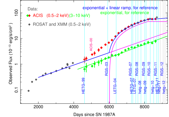
Figure 1: SN 1987A X-ray light curves with grating observation epochs indicated. The 0.5–2 keV data (black, red) show an initial exponential behavior whose slope increases after day $\sim$ 4500 and then decreases from day $\sim$ 6300, possibly leveling off at the recent epoch $\sim$ 8800 days. In constrast, the 3–10 keV flux (green) has more closely followed a consistent exponential behavior to the present. For reference, the sum of an exponential (beginning at day 2000) and a linear ramp increase (from day 6000 to day 8200), is included (magenta, blue) to highlight the general phases of the 0.5–2 keV light curve. The ROSAT fluxes are taken from Haberl et al. (2006) and the ACIS values are from Park et al. (2011).

2 GRATING OBSERVATIONS AND DATA REDUCTION

The grating observations of SN 1987A are listed in Table 1, including those from instruments on Chandra (High- and Low- Energy Transmission Gratings: HETG, LETG) and XMM-Newton (Reflection Grating Spectrometer, RGS). The observation epochs are marked on the SN 1987A light curve of Figure 1, showing that only the HETG-99 observation (Michael et al. 2002) was taken before day 5500 after which the flux from the shock–protrusion collisions became significant. Along with HETG-99, the deep non-grating Chandra ACIS-00 observation at 5036 days (Park et al. 2002, ObsId 1967) gives the best pre-collision X-ray spectra (albeit at only CCD resolution) and is included in the table as well. With the collision getting underway, the RGS-03 (Haberl et al. 2006) and LETG-04 (Zhekov et al. 2005, 2006) observations cover a transition period. Since 2007, with most of the X-ray flux due to the shock-ring interaction, there have been regular grating observations made with both Chandra (Dewey et al. 2008; Zhekov et al. 2009) and XMM-Newton (Sturm et al. 2010).

For our data analysis, we use standard spectral extractions from the observations as described in § 2.1 & § 2.2. The various analyses, described in § 2.3 & § 2.4, are then carried out in ISIS (Houck & Denicola 2000) using a common set of scripts that include some simple tailoring of the energy ranges and spatial-spectral parameters (see Appendix A) based on the type of data, e.g., HETG vs. RGS.

2.1 Chandra Data

Public Chandra grating data and their spectral extractions are available and were obtained from the TGCat archive  (Huenemoerder et al. 2011). All of these had been re-processed in 2010 or later and therefore the downloaded pha, arf and rmf files could be used without any further re-processing. Multiple ObsId’s at the same epoch were combined in ISIS by summing the pha counts, creating an exposure-weighted arf, and summing the exposure times. To reduce background from the less sensitive front-illuminated CCDs, the pha and arf for wavelengths longward of 17.974 Å were set to zero in the plus [minus] order of the MEG [LEG] data. The plus and minus orders are then combined, even though they do have small but significant differences in their line-widths because of the resolved nature of SN 1987A (Zhekov et al. 2005; Dewey et al. 2008). The composite line-shapes are accounted for in the model by a smoothing function that has parameters based on the observed line widths, § 2.3 and Appendix A. In this way we reasonably approximate the combined-orders’ line shapes. Thus, further analysis is carried out on a single spectrum in the case of LETG data and on two spectra (MEG and HEG) for HETG observations.

Some HETG observations are indicated with a lower-case “hetg-YY” designation in the table. These spectra are from the combined “monitoring observations” (PI - David Burrows) in the year 20YY. Starting in 2008 the HETG was inserted for SN 1987A observations in order to reduce the effects of pileup (Park et al. 2011); as a by-product, additional HETG high-resolution data are taken. However, to obtain the shortest exposure times only a subframe of the ACIS is read out; because of this the outer portions of the HETG dispersed “X” pattern (Canizares et al. 2000, 2005) fall outside of the subframe, removing response at longer wavelengths. Instead of centering SN 1987A in the subframe, it is offset in cross-dispersion to get more of the sensitive MEG minus order in the subframe and this extends the response to just include the O VIII line at $\sim$ 0.65 keV.

The most recent HETG observations of SN 1987A, HETG-11 in Table 1, were carried out during 2011 March 1–13 as part of the GTO program (PI - Claude Canizares). The proprietary data were retrieved from the Chandra archive and scripts from TGCat  were used to carry out the spectral extraction using standard CIAO tools; specifically CALDB 4.4.5 and CIAO 4.3 were used to process the data.

The non-grating ACIS-00 observation, ObsId 1967, was downloaded from the archive and processed through level 1 event filtering with CIAO tools. The psextract routine was then used to generate pha, arf, and rmf files for a $\sim$ 6 arc second diameter region around SN 1987A; a background extraction was made but not used because it had very few counts.

2.2 XMM-Newton RGS Data

The European observatory, XMM-Newton, has been used to study SN 1987A at high spectral resolution via its reflection-grating spectrometer, RGS (den Herder et al. 2001). The data and processing steps for the four epochs of RGS data taken through January 2009 have been presented in Sturm et al. (2010). Two subsequent observations, RGS-10 and RGS-11, have been carried out and were similarly processed; XMM-Newton SAS 10.0.0 was used in (re-)processing all RGS data. When read into ISIS the RGS-1 and RGS-2 counts (and backgrounds) are kept separate and jointly fit in further analysis.

Table 1: High-Resolution X-ray Observations of SN 1987A to an Age of 25 Years

	Epoch	ObsId(s)	Expos.	SN Age	$F$(0.47–0.79)		$F$(0.79–1.1)		$F$(1.1–2.1)
Data ID	(year)		(ks)	(days)	(cgs)		(cgs)		(cgs)
HETG-99	1999.76	124, 1387	116.2	4606	0.94	[12%]	0.57	[9%]	0.85	[5%]
ACIS-00	2000.93	1967	98.8	5036	0.67	[2%]	0.71	[2%]	1.01	[2%]
RGS-03	2003.36	0144530101	111.9	5920	4.2		3.6		3.4
LETG-04	2004.66	4640, 5362, 4641, 6099, 5363	288.8	6396	5.4	[2%]	6.2	[2%]	5.2	[1%]
RGS-07	2007.05	0406840301	110.5	7268	10.0		13.8		12.2
HETG-07	2007.23	8523, 8537, 7588, 8538, 7589,	354.9	7335	13.4	[3%]	15.5	[1%]	12.6	[1%]
		8539, 8542, 8487, 8543, 8544,
		8488, 8545, 8546, 7590
LETG-07	2007.69	9581, 9582, 9580, 7620, 7621,	285.2	7503	13.4	[2%]	18.2	[1%]	15.4	[1%]
		9591, 9592, 9589, 9590
RGS-08	2008.03	0506220101	113.7	7627	12.7		18.0		14.5
hetg-08	2008.50	9144	42.0	7799	$\cdots$		19.6	[3%]	18.3	[2%]
RGS-09	2009.08	0556350101	101.4	8012	15.3		22.2		17.9
hetg-09	2009.30	10221, 10852, 10853, 10854,	129.7	8091	$\cdots$		23.2	[2%]	21.2	[1%]
		10855; 10222, 10926
RGS-10	2009.93	0601200101	91.6	8320	16.4		25.2		21.7
hetg-10	2010.46	12125, 12126, 11090;	118.3	8515	$\cdots$		25.0	[2%]	24.8	[1%]
		13131, 11091
RGS-11	2010.93	0650420101	65.7	8687	17.4		29.0		24.9
HETG-11	2011.17	12145, 13238, 13239, 12146	177.7	8774	15.8	[3%]	27.6	[1%]	27.4	[1%]
hetg-11	2011.47	12539; 12540, 14344	101.3	8883	$\cdots$		25.2	[2%]	27.1	[1%]
RGS-12	$\sim$ ’11.92	0671080101	$\sim$ 68	$\sim$ 9048	$\cdots$		$\cdots$		$\cdots$
hetg-12	$\sim$ ’12.22	13735, 14417	$\sim$ 75	$\sim$ 9157	$\cdots$		$\cdots$		$\cdots$

2.3 Fluxes and Three-Shock Model Fitting

The Chandra grating observations can robustly determine the observed flux (and statistical error) in energy bands directly from the data without using a model. Instead of the the usual coarse “flux in the 0.5–2 keV band,” fluxes in Table 1 are given for three bands covering this range. The band boundaries are chosen to avoid strong lines and are dominated by lines of N & O, Fe & Ne, and Mg & Si, respectively. Because of their reduced wavelength coverage the “hetg-YY” data sets do not allow an accurate flux measurement in the lowest-energy band. For the RGS data sets the fluxes given in the table are from 3-shock model fits (described below) because the RGS spectral gaps and background counts complicate a direct-from-the-data approach.

Comparing HETG-11 fluxes to the previous HETG-07 ones shows that the main deviation from the trend of continued flux increase has happened primarily in the lowest energy range: while the 0.79–1.1 and 1.1–2.1 keV fluxes have increased by factors of 1.78 and 2.17, respectively, the 0.47–0.79 keV flux has increased by a smaller factor of only 1.18. Likewise, similar spectral changes are seen in the recent RGS data of 2010 December (“RGS-11”), continuing trends seen earlier; for example, whereas the Ne X flux increased by 36 % from RGS-08 to RGS-09 the lower-energy N VII flux increased by only 10 % in the same period (Sturm et al. 2010).

A nominal non-equilibrium ionization (NEI) model was fit independently to each epoch’s data with the goal of capturing all of the relevant lines in that epoch’s spectrum. In order to allow for the wide range of shock temperatures seen in SN 1987A (Zhekov et al. 2009, Figure 2), the model consists of the sum of three plane-parallel shock components with common (“tied”) abundances. Physically, a single plane-parallel shock model represents the emission from a uniform slab of material into which a shock wave has propagated for some finite time, $t_{s}$ (Borkowski et al. 2001). The shocked portion of the slab has uniform electron temperature, $kT_{e}$, and density, $n_{e}$, but has a linear variation in the time since shock passage, going from $\sim$ 0 immediately postshock to a maximum of $t_{s}$ for the earliest-shocked material. Thus, the plane-parallel shock emission can be parameterized by a normalization ($\propto n_{e}n_{H}V$), the abundances, the postshock electron temperature, and the maximum ionization age , $\tau=n_{e}t_{s}$.

The sum of the three shock components is then smoothed with a Gaussian function to account for line-broadening and the finite size of SN 1987A. Finally, there is an overall photo-electric absorption term to account for Galactic and LMC absorption. The model is implemented in ISIS, making use of the XSPEC spectral models library; the model specification (Expression A1) and a description of the smoothing parameters are given in Appendix A. Many of the model parameters are fixed as in previous work (Zhekov et al. 2009): the column density  ($N_{H}=$ 1.3$\times 10^{21}$ cm^-2), the redshifts (286.5 km s^-1), and the abundances of elements without strong, visible lines (H=1, He=2.57, C=0.09, N=0.56, Ar=0.54, Ca=0.34, Ni=0.62); as previously the solar photospheric abundances of Anders & Grevesse (1989, Table 2) are used as the reference set. There remain the free parameters consisting of 3 normalizations, 3 temperatures, 3 ionization ages, and the abundances of O, Ne, Mg, Si, S, and Fe.

The parameter set was reduced further by fixing the middle temperature at a value near the (logarithmic) center of the emission measure distribution of SN 1987A, $kT_{\rm\,mid}=$ 1.15 keV (Zhekov et al. 2009, Figure 2). Since the $\sim$ 1 keV emission had grown from 2004 to 2007, the expectation, borne out in Tables 2 & 4, is that this component would have a growing contribution to the model, especially at later epochs. To test the (in)sensitivity of the fit values to the exact value of $kT_{\rm\,mid}$, the HETG-11 data were fit with additional $kT_{\rm\,mid}$ values of 1.0 & 1.3 keV. All of the HETG-11 fit parameters showed small variations over the test set of mid-temperature values, {1.0, 1.15, 1.3} keV. Some examples are: $kT_{\rm\,lo}$ takes values {0.50, 0.54, 0.56}, the $kT_{\rm hi}$ norm varies as {2.4, 2.0, 1.5}, the silicon abundance varies as {0.41, 0.39, 0.38}, and the $\chi^{2}$ changed slightly as {1069, 1088, 1111} (for 560 degrees of freedom.) These small, gradual variations demonstrate that the exact choice for the middle temperature is somewhat arbitrary and nearly degenerate with other parameters.

Two more parameters are removed by constraining the ionization ages to cover a factor of 2, e.g., as seen in Zhekov et al. (2009), specifically setting: $\tau_{\rm\,lo}=\sqrt{2}\,\tau_{\rm\,mid}$ and $\tau_{\rm\,hi}=\tau_{\rm\,mid}\,/\sqrt{2}$. Hence, in addition to the abundances there are 6 free parameters: $kT_{\rm\,lo}$, $\tau_{\rm\,mid}$, $kT_{\rm\,hi}$, and the 3 normalizations, $N_{\rm lo},N_{1.15},N_{\rm hi}$. This is the same number of parameters as for a general 2-shock model (2 norms, 2 $kT$’s, 2 $\tau$’s) and gives slightly better fits.

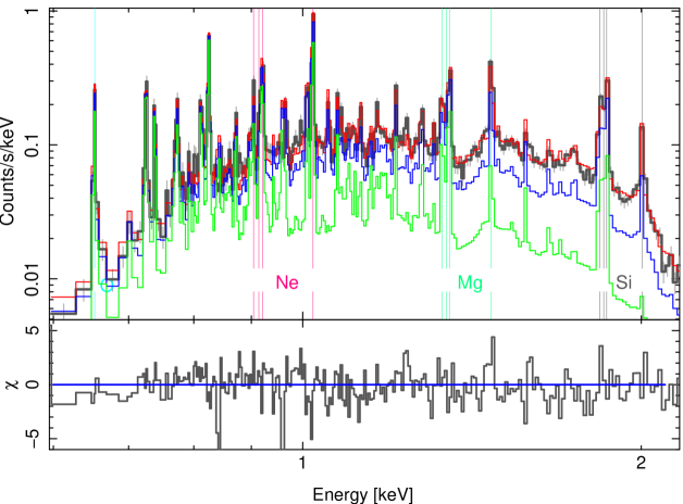
Figure 2: HETG-11 data and model. The data (black) are globally fit by a 3-vpshock model (red). Removing the high-temperature component gives the blue curve and just the low-temperature component is shown in green.

The 3-shock model was fit to the HETG and LETG data in the 0.6 to 5 keV range, giving good overall fits, Figure 2. For fitting, the spectra were binned to a minumum of 20–30 counts per bin and a minimum bin width of $\sim$ 0.05 Å. The HEG data are ignored below 0.78 keV ($>$15.9 Å) and ignored completely for the HETG-99 data. Because of their reduced wavelength coverage, several changes were made for the “hetg-YY” data sets: they were “noticed” in the range 0.69–5 keV for the MEG (1.25–5 keV for the HEG), the O abundance was fixed, and the $kT_{\rm\,lo}$ value was fixed (these latter two were set to values based on the HETG-07 and HETG-11 fits.) The RGS data sets do a good job of covering the N line $\sim$ 0.5 keV but have reduced sensitivity above the Si XIV line, so these data were fit in the range 0.47 to 2.20 keV with the N abundance free, the S abundance frozen at a nominal value (0.36), and the $kT_{\rm\,hi}$ value fixed. The ACIS-00 spectrum was fit over the 0.4 to 8.1 keV range with N free.

The values for the 3-shock fit parameters and their 1-$\sigma$ confidence ranges are given in Table 2. As expected from their low fluxes, the two pre-collision data sets (HETG-99, ACIS-00) show comparatively low normalizations. Note that the RGS values and the HETG/LETG values differ significantly at similar epochs; this is probably due to near-degeneracies in the model which amplify the differences between the spectrometers in terms of their energy-range coverage, statistical weighting (counts vs. energy), and line-spread functions. However they do show the same general trends, e.g., toward larger $\tau_{\rm\,mid}$ values at more recent epochs. In the next section we use these 3-shock fits as good starting points to look for and measure the presence of the v-b component.

Table 2: Parameters of the Global 3-Shock Model Fits

	Normalizations			$kT_{\rm\,lo}$	$\tau_{\rm\,mid}$	$kT_{\rm\,hi}$	—   Relative abundances   —
Data ID	$N_{\rm lo}$	$N_{\rm 1.15}$	$N_{\rm hi}$	(keV)	(10${}^{11}{{\rm s}\over{{\rm cm}^{3}}}$)	(keV)	N	O	Ne	Si	Fe
HETG-99	0.17 $\pm$35%	[0]	0.13 $\pm$12%	[0.74]	2.1 $\pm$342%	[4.3]	[0.56]	0.12 $\pm$286%	0.13 $\pm$185%	0.13 $\pm$135%	0.10 $\pm$160%
ACIS-00	0.18 $\pm$20%	[0]	0.12 $\pm$9%	0.73 $\pm$11%	8.2 $\pm$19%	4.2 $\pm$14%	1.6 $\pm$63%	0.47 $\pm$50%	0.61 $\pm$42%	0.68 $\pm$27%	0.12 $\pm$45%
RGS-03	3.6 $\pm$12%	[0]	0.14 $\pm$5289%	[0.50]	4.1 $\pm$46%	[4.3]	0.24 $\pm$41%	0.053 $\pm$34%	0.11 $\pm$21%	0.42 $\pm$184%	0.027 $\pm$23%
RGS-07	3.0 $\pm$6%	0.35 $\pm$36%	1.1 $\pm$11%	0.51 $\pm$2%	4.8 $\pm$11%	[4.3]	1.1 $\pm$12%	0.15 $\pm$5%	0.47 $\pm$9%	0.61 $\pm$19%	0.28 $\pm$7%
RGS-08	3.4 $\pm$3%	0.72 $\pm$15%	1.3 $\pm$2%	0.52 $\pm$2%	4.7 $\pm$1%	[2.7]	1.1 $\pm$4%	0.15 $\pm$4%	0.40 $\pm$7%	0.37 $\pm$21%	0.30 $\pm$5%
RGS-09	5.3 $\pm$3%	1.4 $\pm$9%	1.2 $\pm$12%	0.53 $\pm$1%	7.9 $\pm$6%	[2.7]	1.2 $\pm$0%	0.17 $\pm$0%	0.44 $\pm$5%	0.35 $\pm$19%	0.25 $\pm$3%
RGS-10	5.1 $\pm$3%	1.6 $\pm$7%	1.5 $\pm$0%	0.54 $\pm$1%	10 $\pm$0%	[2.7]	1.5 $\pm$0%	0.20 $\pm$0%	0.53 $\pm$5%	0.57 $\pm$7%	0.29 $\pm$2%
RGS-11	4.7 $\pm$3%	1.3 $\pm$0%	2.1 $\pm$6%	0.57 $\pm$1%	15 $\pm$0%	[2.7]	2.0 $\pm$0%	0.31 $\pm$0%	0.76 $\pm$0%	0.61 $\pm$16%	0.39 $\pm$2%
LETG-04	2.3 $\pm$4%	0.64 $\pm$10%	0.28 $\pm$8%	0.48 $\pm$2%	3.7 $\pm$8%	5.3 $\pm$9%	[0.56]	0.090 $\pm$9%	0.26 $\pm$6%	0.30 $\pm$6%	0.13 $\pm$6%
HETG-07	5.2 $\pm$1%	1.7 $\pm$2%	0.64 $\pm$2%	0.47 $\pm$0%	3.4 $\pm$0%	4.3 $\pm$1%	[0.56]	0.096 $\pm$0%	0.22 $\pm$0%	0.31 $\pm$0%	0.16 $\pm$0%
LETG-07	5.2 $\pm$2%	1.4 $\pm$2%	1.2 $\pm$2%	0.48 $\pm$1%	3.7 $\pm$4%	2.4 $\pm$1%	[0.56]	0.090 $\pm$3%	0.27 $\pm$2%	0.34 $\pm$1%	0.19 $\pm$2%
hetg-08	6.6 $\pm$7%	1.6 $\pm$37%	1.5 $\pm$31%	[0.52]	3.6 $\pm$18%	2.4 $\pm$18%	[0.56]	[0.11]	0.20 $\pm$10%	0.32 $\pm$8%	0.14 $\pm$10%
hetg-09	5.5 $\pm$6%	2.2 $\pm$10%	1.6 $\pm$9%	[0.52]	5.9 $\pm$12%	2.7 $\pm$6%	[0.56]	[0.11]	0.30 $\pm$7%	0.37 $\pm$5%	0.22 $\pm$5%
hetg-10	5.9 $\pm$7%	2.8 $\pm$14%	1.9 $\pm$16%	[0.52]	5.7 $\pm$13%	2.7 $\pm$12%	[0.56]	[0.11]	0.27 $\pm$9%	0.37 $\pm$5%	0.19 $\pm$5%
HETG-11	6.2 $\pm$1%	3.1 $\pm$0%	2.0 $\pm$0%	0.54 $\pm$1%	7.0 $\pm$0%	2.7 $\pm$0%	[0.56]	0.12 $\pm$0%	0.30 $\pm$0%	0.39 $\pm$0%	0.20 $\pm$0%
hetg-11	4.9 $\pm$8%	3.5 $\pm$14%	1.9 $\pm$21%	[0.54]	7.9 $\pm$18%	3.1 $\pm$19%	[0.56]	[0.12]	0.32 $\pm$9%	0.40 $\pm$5%	0.20 $\pm$6%

Note. — Parameter values are followed by an indication of their $\pm$ 1-$\sigma$ statistical confidence range, $c_{\rm lo}$ to $c_{\rm hi}$, given as a percentage: $100(\sqrt{c_{\rm hi}/c_{\rm lo}}-1$). A bracketed parameter value indicates that it has been fixed at that value during fitting; these fixed values are generally based on other datasets’ results. $N_{\rm 1.15}$ is not used (set to 0) for the three earliest data sets, due to their lower total source counts. $kT_{\rm\,lo}$ is fixed for the HETG-99, RGS-03, and the “hetg” datasets which have reduced low-energy counts or coverage. $kT_{\rm\,hi}$ is fixed for the RGS and HETG-99 datasets because of reduced high-energy coverage and counts. The N abundance is only fit for the RGS and ACIS-00 datasets, and the O abundance is fixed for the “hetg” datasets which have reduced low-energy coverage and counts.

2.4 The Very-Broad Component and Its Evolution

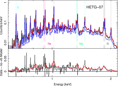
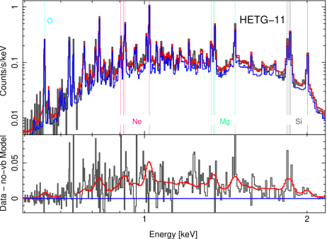
Figure 3: Deep HETG spectra and their very-broad (v-b) models. The HETG-07 (top pair) and HETG-11 (bottom pair) data are shown (black) with the best-fit v-b 3-shock model (red). The non-broad model component is shown as well (blue). The lower half plots show the difference (black) between the data and the non-broad component with the v-b component over plotted (red).

To look for and quantify a v-b line component in the SN 1987A spectra we start with the data and 3-shock model fits (above) and extend the model to include a v-b component that is a broadened version of the 3-shock model itself; the model definition is explicitly given in Appendix A, Expression A2. The v-b extension adds two additional parameters: the fraction of the total flux that is in the v-b component ($f_{\mathrm{v}\textrm{\footnotesize-}\mathrm{b}}$) and the width of the v-b component expressed as an equivalent FWHM in velocity ($v_{\mathrm{v}\textrm{\footnotesize-}\mathrm{b}}$).

The choice of broadening the whole spectrum is the simplest given the low signal-to-noise ratio of the v-b component in any given line, provided there is some expectation that the bright lines of the v-b component are similar to those of the narrow emission. At face value this may seem to be unlikely, with the v-b lines produced by a plasma with very different temperatures and ionization ages from the plasma producing the narrow lines. However, our hydrodynamic modeling shows that the approximation is a surprisingly good one as seen in Figure 14 and discussed in § 4.5. However, based on this comparison we have chosen to ignore the Fe XVII 0.70–0.75 keV range when doing v-b fitting (below) as it is the only bright line-complex that is not predicted to have a v-b component.

The v-b–3-shock model is fit to the data using $\sim$ 60% finer binning and a somewhat smaller energy range that focusses on the brightest, high-resolution lines in the particular spectra, generally those of O, Ne, Mg, Si, and Fe-L. For HETG, LETG and RGS data these ranges are, respectively: 0.62–2.1 keV, 0.6–1.6 keV (no Si), and 0.47–1.1 keV (including N but not Mg and Si). For “hetg-YY” data sets because of their limited low-energy range, the O line is not included and the O abundance is frozen at the average of the HETG-07 and HETG-11 O v-b values. Because of the reduced energy range of the v-b fitting, the $kT_{\rm\,lo}$, $\tau_{\rm\,mid}$ and $kT_{\rm\,hi}$ parameters were fixed at their 3-shock values; this leaves the 3 normalizations and the abundances to be fit along with the v-b fraction and width.

As examples, the v-b fits to the HETG-07 and HTEG-11 data are shown in Figure 3; note that the y-axes of the lower, difference plots are the same, showing that the v-b flux is increasing in absolute terms. The statistics of this v-b fitting are given in the left-half of Table 3; in particular the values of $F_{2}$ are large enough to indicate that the addition of the two v-b parameters has improved the model fit significantly.

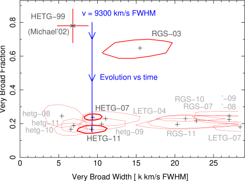
Figure 4: Confidence contours for the very-broad component parameters. Solid curves give the 68 % ($\Delta\chi^{2}=2.3$) contours for fits to each grating data set; the best-fit values are indicated with “$+$”’s. The two deep HETG observations, HETG-07 & HETG-11, show a similar, well-determined v-b width of $\sim$ 9300 km s^-1 FWHM. See the text for a discussion of the spread seen among the contours.

Instead of tabulating the best-fit v-b parameters and their ranges, it is more useful to generate two-dimensional confidence contours in “v-b fraction vs. v-b width” space. These contours and their best-fit values are shown in Figure 4; for HETG-99 the data point with errors is based on the 2-Gaussian “stacked fitting” result given in Michael et al. (2002). The earliest data sets, HETG-99 and RGS-03, show large values of v-b fraction ($>$ 0.6) with widths of order 10$\times 10^{3}$ km s^-1. In contrast the later observations show v-b fractions within the range 0.15 to 0.30 and cover a large spread in widths, with the HETG values below 15$\times 10^{3}$ km s^-1 and RGS-determined widths above this value.

This separation suggests that the measurement of the v-b component depends on the particular spectrometer used. Figure 5 shows how the spectrometers “see” a monochromatic line consisting of a narrow and a v-b-component; these plots include SN 1987A’s spatial-spectral blur descibed in Appendix A. The HETG, even at the higher Mg XII energy, clearly separates the narrow and v-b components, although it’s also clear that the v-b presence is subtle. For the LETG the narrow component is significantly broadened by the spatial extent of SN 1987A and at high energies the v-b component is almost completely covered by the narrow component. The RGS line-spread function is more peaked than the LETG at O VIII, however it includes extended wings so that even the narrow component produces counts far from the line center. Hence the RGS v-b measurement will be particularly sensitive to the accuracy of its LSF calibration.

With these considerations in mind, we see that the two deep HETG observations, HETG-07 and HETG-11, should give the most accurate measure of the v-b component. Comparing their small confidence contours, there is a clear change in the v-b fraction from 2007 to 2011. In terms of the v-b width, these two HETG contours show very similar values of $\approx$ 9300 km s^-1 FWHM, with an estimated 90 % confidence range of $\pm$ 2000 km s^-1. This value is also in rough agreement with the (lower statistics) HETG-99 and RGS-03 widths and so it is reasonable to postulate a constant v-b width with a fraction that changes over time as shown by the blue path in Figure 4.

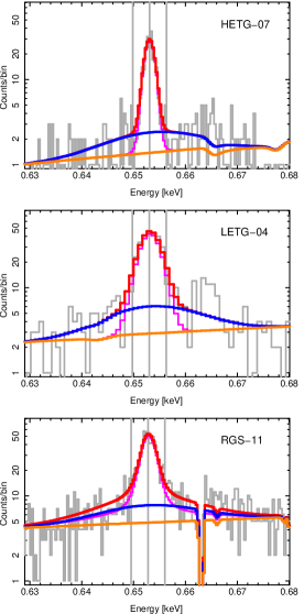
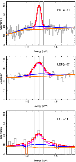
Figure 5: Comparing the grating spectrometer line responses when observing SN 1987A. The HETG(MEG), LETG, and RGS views of the same combination of a narrow line plus a very-broad component are shown for the case of $f_{\mathrm{v}\textrm{\footnotesize-}\mathrm{b}}=25$% and $v_{\mathrm{v}\textrm{\footnotesize-}\mathrm{b}}=9300$ km s^-1 FWHM. Because the resolution varies with energy, responses are shown for O VIII (left colum) and for Mg XII (right column). On each plot the orange curve shows a continuum level, the blue curve is the continuum plus the v-b component, the magenta curve is the continuum plus the narrow component, and the red curve is the sum of all three. Vertical gray lines indicate the line center and $\pm$ 1500 km s^-1 from it. For reference, example data are shown in the background by the light gray histograms; the O VIII region includes the He-like L-$\beta$ line at $\sim$ 0.665 keV. The HETG provides the best separation of the v-b and narrow components especially at the higher energies.

Table 3: Very-Broad Fitting Statistics and Results

	$N_{\rm data}$				—  $v_{\mathrm{v}\textrm{\footnotesize-}\mathrm{b}}\,=$ 9300 km s-1 FWHM  —
Data ID	$-N_{\rm free}$	$\chi^{2}_{\mathrm{v}\textrm{\footnotesize-}\mathrm{b}}$	$\Delta\chi^{2}_{2}$	$F_{2}$	$\Delta\chi^{2}_{1}$	$F_{1}$	$f_{\mathrm{v}\textrm{\footnotesize-}\mathrm{b}}$  &  $1$-$\sigma$ range
HETG-99	32$-$9	24.0	2.0	1.0	1.2	1.1	0.372	0.02 – 0.63
RGS-03	226$-$8	352.7	86.0	26.6	80.0	48.9	0.655	0.61 – 0.70
LETG-04	130$-$9	174.3	68.6	23.8	66.9	46.4	0.248	0.22 – 0.28
RGS-07	216$-$9	360.5	36.3	10.4	31.0	17.7	0.175	0.14 – 0.20
HETG-07	622$-$10	1146.1	347.8	92.9	$\cdots$	$\cdots$	0.244	0.23 – 0.26
LETG-07	140$-$9	355.2	81.7	15.1	48.6	16.5	0.150	0.13 – 0.17
RGS-08	231$-$9	450.3	71.6	17.6	45.7	21.4	0.181	0.16 – 0.21
hetg-08	146$-$9	174.4	28.9	11.4	26.4	20.6	0.254	0.21 – 0.30
RGS-09	217$-$9	416.1	68.9	17.2	33.7	15.6	0.158	0.13 – 0.18
hetg-09	349$-$9	546.6	76.3	23.7	75.0	46.7	0.208	0.18 – 0.23
RGS-10	222$-$9	404.0	81.2	21.4	66.8	34.2	0.206	0.18 – 0.23
hetg-10	328$-$9	427.0	44.5	16.6	42.4	31.6	0.178	0.15 – 0.20
RGS-11	201$-$9	429.6	67.1	15.0	57.5	25.2	0.211	0.19 – 0.24
HETG-11	599$-$10	1115.3	116.7	30.8	$\cdots$	$\cdots$	0.173	0.16 – 0.19
hetg-11	319$-$9	422.0	47.2	17.3	45.1	33.1	0.201	0.17 – 0.23

Note. — The four left-most numerical columns give values related to the very-broad fitting of the data sets: the number of data bins minus the number of free fit parameters, the $\chi^{2}$ value for the v-b fit, the amount by which $\chi^{2}_{\mathrm{v}\textrm{\footnotesize-}\mathrm{b}}$ is an improvement over (less than) the non-v-b $\chi^{2}$ value, and the $F$-statistic for adding the 2 v-b degrees of freedom to the model. Specifically, $F_{2}=(\Delta\chi^{2}_{2}/2)/(\chi^{2}_{\mathrm{v}\textrm{\footnotesize-}\mathrm{b}}/(N_{\rm data}-N_{free}))$ and values of $F_{2}$ greater than $F_{\rm crit}\approx$ 7.3 indicate a high confidence, $>0.999$, that the addition of the 2 v-b parameters does result in a significantly improved model.

The right-most four columns give values related to a constrained v-b fitting where the v-b velocity width is fixed at the HETG-07/HETG-11 average value; thus there is only a single free v-b parameter: $f_{\mathrm{v}\textrm{\footnotesize-}\mathrm{b}}$, the v-b fraction. The first two of these columns give the $\chi^{2}$ improvement and the appropriate $F$-statistic: $F_{1}=(\Delta\chi^{2}_{1}/1)/(\chi^{2}_{9300}/(N_{\rm data}-N_{free}+1))$ with $\chi^{2}_{9300}=\chi^{2}_{\mathrm{v}\textrm{\footnotesize-}\mathrm{b}}+\Delta\chi^{2}_{2}-\Delta\chi^{2}_{1}$. In this case we have $F_{\rm crit}\approx$ 11.4. The right-most two columns give the best-fit v-b fraction and its 1-$\sigma$ confidence range for the constrained fitting.

Given the above, we fix the width of the v-b component at $v_{\mathrm{v}\textrm{\footnotesize-}\mathrm{b}}=9300$ km s^-1 FWHM and fit for just the v-b fraction. The results of this “constrained” fitting are given in the right-half of Table 3, including the v-b fractions and their 68 % confidence ranges. Note that for most data sets the $\chi^{2}$ change when doing this constrained fitting, $\Delta\chi^{2}_{1}$, is a substantial portion of the $\chi^{2}$ change when the v-b width is also being fit, $\Delta\chi^{2}_{2}$. This suggests that the data do not strongly constrain the width to differ from our assigned value; the elongated contours of Figure 4 suggest this as well. Conversely, the v-b fractions given by the constrained fitting have only a small dependence on the assigned width. As examples, when the data sets LETG-07, RGS-11, HETG-11, and hetg-11 were fit with the width set to 6500 & 13000  km s^-1 FWHM, the best-fit fractions found are: 0.132 & 0.160, 0.216 & 0.210, 0.163 & 0.178, and 0.200 & 0.188, respectively. These variations are actually within the statistical 1-$\sigma$ ranges given for the $f_{\mathrm{v}\textrm{\footnotesize-}\mathrm{b}}$ values in Table 3, and so the choice of the v-b width will not significantly change the v-b fractions and light curve.

Having determined the v-b fractions for the data sets we can now re-do the 3-shock fitting of § 2.3 with the appropriate v-b component fixed and included in the model. This gives the results in Table 4. Note that the abundances have increased compared to the non–v-b values in Table 2. This is expected since a larger flux in a given line is now needed in order to match the height of the narrow-line component in the high-resolution spectrum. The change is especially pronounced for HETG-99 where the v-b fraction is 0.78 and the abundances are now in better agreement with those of ACIS-00 (although there is a large error range.) Also as expected, the ACIS-00 values hardly change when the v-b component is included because the lower-resolution CCD spectra are primarily determined by the total line flux with little sensitivity to any underlying velocity structure.

Table 4: Parameters of the Global 3-Shock-with-Very-Broad-Component Model Fits

	Normalizations			$kT_{\rm\,lo}$	$\tau_{\rm\,mid}$	$kT_{\rm\,hi}$	—   Relative abundances   —
Data ID	$N_{\rm lo}$	$N_{\rm 1.15}$	$N_{\rm hi}$	(keV)	(10${}^{11}{{\rm s}\over{{\rm cm}^{3}}}$)	(keV)	N	O	Ne	Si	Fe
HETG-99	0.10 $\pm$54%	[0]	0.12 $\pm$9%	[0.74]	9.2 $\pm$211%	[4.2]	[0.56]	0.82 $\pm$214%	0.77 $\pm$154%	0.45 $\pm$120%	0.26 $\pm$144%
ACIS-00	0.18 $\pm$40%	[0]	0.12 $\pm$9%	0.73 $\pm$13%	8.2 $\pm$69%	4.2 $\pm$17%	1.6 $\pm$142%	0.47 $\pm$25%	0.61 $\pm$73%	0.68 $\pm$43%	0.12 $\pm$24%
RGS-03	1.5 $\pm$21%	[0]	0.17 $\pm$91%	0.57 $\pm$8%	3.0 $\pm$24%	[4.3]	0.86 $\pm$29%	0.16 $\pm$23%	0.28 $\pm$16%	0.68 $\pm$145%	0.11 $\pm$25%
RGS-07	2.4 $\pm$7%	0.16 $\pm$64%	1.0 $\pm$10%	0.52 $\pm$2%	5.2 $\pm$8%	[3]	1.6 $\pm$7%	0.21 $\pm$6%	0.64 $\pm$8%	0.81 $\pm$15%	0.36 $\pm$6%
RGS-08	2.6 $\pm$2%	0.40 $\pm$21%	1.2 $\pm$6%	0.53 $\pm$2%	5.7 $\pm$1%	[2.7]	1.9 $\pm$3%	0.25 $\pm$4%	0.62 $\pm$7%	0.54 $\pm$20%	0.43 $\pm$4%
RGS-09	4.3 $\pm$3%	0.86 $\pm$9%	1.4 $\pm$9%	0.54 $\pm$1%	8.1 $\pm$8%	[2.7]	1.6 $\pm$5%	0.23 $\pm$2%	0.57 $\pm$6%	0.44 $\pm$18%	0.33 $\pm$4%
RGS-10	3.8 $\pm$4%	0.98 $\pm$15%	1.6 $\pm$9%	0.55 $\pm$1%	12 $\pm$3%	[2.7]	2.5 $\pm$4%	0.33 $\pm$3%	0.80 $\pm$5%	0.81 $\pm$10%	0.42 $\pm$3%
RGS-11	3.4 $\pm$2%	0.68 $\pm$16%	2.1 $\pm$8%	0.57 $\pm$2%	17 $\pm$8%	[2.7]	3.3 $\pm$2%	0.49 $\pm$1%	1.2 $\pm$5%	0.93 $\pm$14%	0.59 $\pm$0%
LETG-04	1.8 $\pm$6%	0.41 $\pm$11%	0.34 $\pm$7%	0.50 $\pm$3%	4.3 $\pm$4%	4.5 $\pm$14%	[0.56]	0.14 $\pm$10%	0.38 $\pm$7%	0.40 $\pm$7%	0.18 $\pm$5%
HETG-07	3.9 $\pm$2%	0.60 $\pm$3%	1.1 $\pm$1%	0.50 $\pm$1%	3.4 $\pm$2%	3.0 $\pm$1%	[0.56]	0.15 $\pm$4%	0.33 $\pm$2%	0.41 $\pm$2%	0.22 $\pm$2%
LETG-07	4.6 $\pm$2%	0.84 $\pm$3%	1.5 $\pm$4%	0.49 $\pm$2%	3.8 $\pm$2%	2.3 $\pm$3%	[0.56]	0.11 $\pm$3%	0.33 $\pm$2%	0.39 $\pm$3%	0.22 $\pm$2%
hetg-08	5.6 $\pm$9%	0.54 $\pm$189%	1.9 $\pm$25%	[0.52]	4.1 $\pm$15%	2.2 $\pm$15%	[0.56]	[0.15]	0.32 $\pm$9%	0.42 $\pm$6%	0.19 $\pm$11%
hetg-09	4.5 $\pm$6%	1.2 $\pm$23%	1.9 $\pm$10%	[0.52]	5.5 $\pm$13%	2.6 $\pm$6%	[0.56]	[0.15]	0.41 $\pm$8%	0.46 $\pm$6%	0.28 $\pm$6%
hetg-10	5.2 $\pm$7%	1.9 $\pm$22%	2.2 $\pm$15%	[0.52]	5.7 $\pm$17%	2.6 $\pm$9%	[0.56]	[0.15]	0.35 $\pm$9%	0.46 $\pm$6%	0.23 $\pm$7%
HETG-11	5.3 $\pm$2%	2.2 $\pm$1%	2.2 $\pm$1%	0.55 $\pm$1%	7.2 $\pm$2%	2.8 $\pm$2%	[0.56]	0.15 $\pm$7%	0.40 $\pm$2%	0.49 $\pm$2%	0.26 $\pm$2%
hetg-11	4.1 $\pm$9%	2.4 $\pm$19%	2.3 $\pm$15%	[0.55]	7.7 $\pm$29%	2.8 $\pm$11%	[0.56]	[0.15]	0.45 $\pm$14%	0.51 $\pm$9%	0.26 $\pm$7%

Note. — The data sets have been fit as before, Table 2, with the inclusion of a v-b component fixed to have FWHM = 9300 km s^-1 and a fraction as given in Table 3.

Parameter values are followed by an indication of their $\pm$ 1-$\sigma$ statistical confidence range, $c_{\rm lo}$ to $c_{\rm hi}$, given as a percentage: $100(\sqrt{c_{\rm hi}/c_{\rm lo}}-1$). A bracketed parameter value indicates that it has been fixed at that value during fitting; these fixed values are generally based on other datasets’ results. $N_{\rm 1.15}$ is not used (set to 0) for the three earliest data sets, due to their lower total source counts. $kT_{\rm\,lo}$ is fixed for the HETG-99 and the “hetg” datasets which have reduced low-energy counts or coverage. $kT_{\rm\,hi}$ is fixed for the RGS and HETG-99 datasets because of reduced high-energy coverage and counts. The N abundance is only fit for the RGS and ACIS-00 datasets, and the O abundance is fixed for the “hetg” datasets which have reduced low-energy coverage and counts.

3 HYDRODYNAMIC MODELING OF SN 1987A

Besides being an extremely well-studied object, SN 1987A has been frequently modelled in almost every wavelength regime. The earliest calculations, which delineated the circumstellar material (CSM) into a low-density inner and high-density outer region, were made by Itoh et al. (1987). The X-ray emission was modelled by Masai et al. (1991) and Luo & McCray (1991a) using 1-dimensional (1D) models. Two-dimensional (2D) models were explored by Luo & McCray (1991b) for the case of an hour-glass equatorial ring (ER) structure. Suzuki et al. (1993) carried out 2D axisymmetric smoothed particle hydrodynamics (SPH) simulations with the ER modeled as a torus; their Figures 4–8 demonstrate the hydrodynamic complexity by showing the different components’ spatial distributions. Masai & Nomoto (1994) went back to the 1D models but took into account the light-travel times from different parts of the remnant. Luo et al. (1994) carried out 2D calculations approximating the ER as a rigid boundary; they also introduced the ejecta density distribution that has been subsequently used by most authors, and forms the basis for the ejecta density profile used in this paper.

The increasing X-ray and radio emission led Chevalier & Dwarkadas (1995) to propose the existence of an ionized H II region interior to the ER. The FS had collided with this region around day 1200, and was expanding in this moderately-high density medium, $\rho\approx 100$ amu cm^-3, giving rise to increasing X-ray and radio emission. The slowing down of the shock wave observed at radio wavelengths was consistent with this conjecture. The X-ray flux from the H II region was modelled by Borkowski et al. (1997a), whereas a detailed prediction of the expected X-ray flux and spectrum when the shock collided with the dense ER was given in Borkowski et al. (1997b).

For the next decade or so, investigations of the X-ray emission were mainly made via simpler, non-hydrodynamical models that attempted to tie in the observed X-ray emission to the CSM properties (Park et al. 2004, 2005, 2006; Haberl et al. 2006; Zhekov et al. 2010). Dwarkadas (2007a) revised the older simulations made (but not presented) in Chevalier & Dwarkadas (1995) using more recent data, and managed to create spherically symmetric hydrodynamical models that successfully reproduced the FS radius and velocity as measured at radio frequencies. Using these simulations he was also able to make a crude estimate of the X-ray light curve. This model was updated in Dwarkadas (2007b), and forms the basis of the hydrodynamical simulations that are presented in the following.

3.1 Our Hydrodynamic Model of SN 1987A

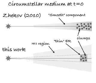
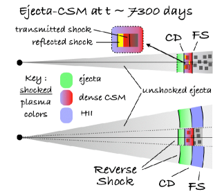
Figure 6: Schematic diagrams of the CSM as modeled in Zhekov et al. (2010), top row, and in this work, bottom row. The left diagrams show the CSM configuration assumed at the time of the SN explosion. The coresponding diagrams at the right show the configuration $\sim$ 7300 days after explosion when the forward shock, driven by the expanding ejecta, has progressed into the dense, clumpy ER. The Zhekov model is based on a single 1D hydrodynamics whereas our model consists of two 1D models, one that includes the dense ER and one that accounts for the H II material above and below the equatorial plane. It is this latter component that gives rise to the very-broad X-ray emission.

The structure of the CSM around SN 1987A is inherently 3-dimensional, as is visible in the amazing images from the Hubble Space Telescope, most recently in Larsson et al. (2011). Modelling the ejecta-CSM interaction in 3-dimensions is a highly challenging and computationally demanding problem, does not encourage iterative parameter exploration, and requires multi-dimensional non-equilibrium ionization (NEI) X-ray emission calculations. However, given the substantial symmetries in the overall geometry, it is possible to partition the domain into one or more regions whose emission can then be approximated by a spherically symmetric 1D simulation. These simulations can then be summed together, weighted by the fraction of the full $4\pi$ solid angle that they each subtend.

As examples of this approach we show schematics in Figure 6 for the modeling of Zhekov et al. (2010) and our model. The former consists of a single 1D solution with a smooth, increasing-density CSM component. To match the observed spectra, especially at late times, dense “clumps” are included in the CSM with the clump X-ray emission based on transmitted and reflected shock equations (Zhekov et al. 2009). Our model in the lower portion of Figure 6 is motivated by the on-going existence of the v-b component which requires a combination of two 1D solutions:

• A “with ER” simulation that consists of an H II region followed at larger radii by a density jump to high values at the ER location; the density profile is shown in Figure 7. This component subtends a small solid angle, $\Omega_{\rm ER}$, and the high-density ER includes additional “clumping” (§  4.2 & 4.4). This component is similar to the 1D model of Zhekov et al. (2010).

• A “no ER” simulation in which the H II region continues to large radii and there is no ER density jump. This simulation produces the v-b emission and corresponds to material above and below the equatorial plane; it subtends a moderate solid angle, $\Omega_{\mathrm{H\,II}}$.

This multi-1D technique does have its limitations, especially for the “with ER” case, and we will keep these in mind.

The simulations here were carried out using the VH-1 code, a 1, 2, and 3-dimensional finite-difference hydrodynamic code based on the Piecewise Parabolic Method (Colella & Woodward 1984). The code solves the hydrodynamical equations in a Lagrangian framework, followed by a remap to the original Eulerian grid. Radiative cooling is included in the form of the X-ray cooling function scaled by a factor of 3.5 to account for IR dust emission, $L_{\mathrm{IR}}/L_{\mathrm{X}}\approx 2.5$.

For each of a set of time steps, the code outputs a snapshot file giving the hydrodynamic quantities density, velocity, and pressure at each radial zone; two examples are shown in Figure 8. The set of snapshot files is then processed by custom routines coded in S-Lang  and run within the ISIS software environment. The radial grid is rebinned into mass cuts, so that the time evolution of each parcel of gas in a given mass shell can be accurately followed; in this way the NEI state is tracked and the X-ray emission can be calculated (Dwarkadas et al. 2010).

Of course we did not simply pick parameters, run the simulation, and have agreement with observations. An iterative process of trial & error was carried out to converge on model parameters that reproduced the various measured properties of SN 1987A, especially in the X-ray. Rather than take the reader through these steps (and mis-steps), we summarize in the following sections the final model properties and then compare the model results to data in § 4.

3.2 Ejecta Parameters

The ejecta are modelled using the Chevalier (1982) prescription where the ejecta are in homologous expansion with a density that decreases as a power-law with radius, i.e.,

$$\rho_{\rm ej}=C~{}t^{-3}\,(r/t)^{-n}~{}.$$ (1)

This is written to show that one can also consider the density profile as a function of $v=r/t$. Since a power-law extending all the way back to the origin is unphysical, below a certain velocity, $v_{t}$, the density is assumed to be a constant, see the “Ejecta” portion of the density in Figure 7. Thus the profile can be specified by the three parameters: $C$, $n$, and $v_{t}$ . The ejecta’s total kinetic energy and mass are functions of these parameters (Chevalier & Liang 1989, equ. 2.1) and so we can equivalently choose other 3-parameter sets, e.g.: $n$, $E_{\rm ej}$, and $M_{\rm ej}$ .

In our 1D hydrodynamic simulations, the RS moves into the ejecta and at most shocks only the outer $\sim$ 0.5 solar masses of the ($4\pi$) ejecta profile, at which point the ejecta velocity is $\sim$ 5700 km s^-1. Provided that $v_{t}$ is less than this value, which is generally the case, we are insensitive to the plateau transition location. Our simulations then only depend on the outer profile, that is the two parameters of Equation 1: the normalization of the power-law profile ($C=$ 2.03$\times 10^{85}$ g cm⁶ s^-6)  and the exponent ($n=9$ from Luo & McCray (1991b)). Implicitly fixing these two, we are then left with a degenerate degree of freedom, our insensitivity to $v_{t}$, in choosing the ejecta parameters. Hence there are pairs of ($E_{\rm ej}$, $M_{\rm ej}$) that will equivalently give the hydrodynamics presented here: (2.4, 16), (1.5, 7.9), or (1.0, 4.3), where the energy is in units of 10⁵¹ erg and the mass is in solar masses. It’s important to note that we do not make any determination of the actual global values of these parameters, they are only used to define the outer ejecta properties relevant to our hydrodynamics.

3.3 H II Region Parameters

Estimates of the parameters of the H II region are determined mainly from observations. This was first done by Lundqvist (1999) by analyzing the ultraviolet line emission from SN 1987A. Dwarkadas (2007a, b) attempted to refine these parameters by calculating the radius and velocity of the expanding SN shock wave in a spherically symmetric case, comparing the results to radio observations, and iterating until a good fit was obtained. They also calculated a reasonable fit to the hard X-ray emission under collisional-ionization equilibrium (CIE) conditions.

In the present work we further develop these earlier calculations. The H II region radius and density profile are adjusted so that our simulated emission agrees with the early X-ray light curves (up to day $\sim$ 5000); in particular, producing a reasonably sharp “turn-on” at $\sim$ 1400 days and agreeing with the HETG-99 and ACIS-00 measured spectra at later times. A further constraint on the H II region, especially near the equatorial plane, comes from the requirement that the FS reaches the ER (and/or protrusions) at a time and radius in agreement with the X-ray imaging observations (Racusin et al. 2009). The parameters we have found appropriate for the H II region, shown in Figures 7, have it beginning at 3.61$\times 10^{17}$ cm (0.117 pc) with a density of $\sim$ 130 amu cm^-3 and gradually increasing to $\sim$ 250 amu cm^-3 at 6.17$\times 10^{17}$ cm (0.20 pc) and remaining at this density to larger radii. These X-ray-based values have an inner radius closer to the expectations of Chevalier & Dwarkadas (1995) and differ from the previous H II values (Dwarkadas 2007b, beginning at 4.3$\times 10^{17}$ cm with $\rho\approx 6$ amu cm^-3, increasing to $\rho\approx 200$ amu cm^-3 at 6.2$\times 10^{17}$ cm) which were based primarilly on the radio size at early time; we discuss the reconciliation of these further in § 4.1 and § 4.7.

3.4 Equatorial Ring Parameters

Unlike the H II region where the simple 1D approximation may suffice, it is clear that only a far cruder approximation to the X-ray emitting ER can be made with simple 1D constructs. Note that in this paper we often use the term “ER” as a generic term to refer to the dense ($\sim$ 10⁴ amu cm^-3) equatorial material with which the SN shock interacts. The ER therefore includes the finger-like extensions that McCray (2007) has postulated as extending inwards from the ring. Consequently, the ER is not located at any single radius; this is clearly demonstrated by the gradually increasing number of optical hot spots (Sugerman et al. 2002). A superposition of ER collisions in time is thus expected to make up the ER contribution to the X-ray light curve.

For modeling purposes we choose a single location of the ER starting at a radius of 5.4$\times 10^{17}$ cm (with a density of $\sim$ 9000 amu cm^-3). As we’ll see, this choice reproduces the “kink” in the measured X-ray radius vs time (§ 4.1) and the bulk of the dramatic soft X-ray increase after day 6000 (§ 4.2); hence this model component is representative of the majority of shocked ER material. Since there is an indication that the X-ray flux may be leveling off (Park et al. 2011) we also consider the case of a finite or “thin” ER with a density that then drops from $\sim$ 10800 amu cm^-3  to (a lower, arbitrary value of) $\sim$ 1200 amu cm^-3 at a radius of 5.77$\times 10^{17}$ cm, as shown in Figure 7.

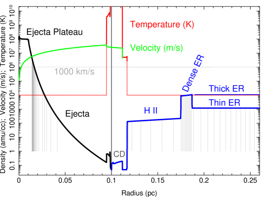
Figure 7: Initial 1D model radial profiles. This early-time ($\sim$ 900 d) configuration shows the ejecta, the H II region, and the options of a “thick” or “thin” ER. The ejecta (black) and CSM (blue) densities are separated at the contact discontinuity (CD); the mean plasma temperature (red) and velocity (green) are also plotted. The gray vertical lines indicate the boundaries of the mass-shells that are tracked and used to compute the NEI X-ray emission; note that they do not need to extend into the plateau region of the ejecta profile.

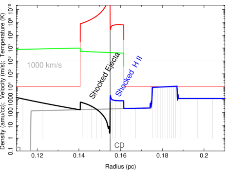
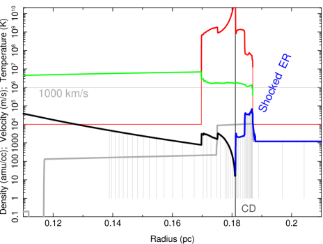
Figure 8: Model profiles at later times. Top: The simulation at the ACIS-00 epoch when the FS has moved well into the H II region; note that the early-time density profile is shown in gray for reference. Bottom: At the HETG-11 epoch, the FS has encountered the “thin ER”, slowed, and is just about to exit the ER. The color coding is the same as for Figure 7.

4 MODEL RESULTS AND COMPARISONS

The previous section summarized the ejecta-CSM properties of our hydrodynamic simulations. In the following we compare several results derived from the simulations with the observed properties of SN 1987A.

4.1 Model Locations

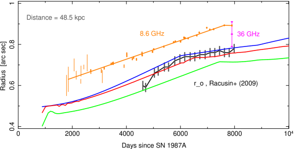
Figure 9: Model radii compared with X-ray and radio measurements. Top: The “with ER” simulation has most X-ray emission between the FS (blue) and CD (red) radii and their locations agree very well with the ACIS-measured average radii (black). Note how the kink due to the ER collision occurs first in the FS curve (around day 6000) and then at later times in the CD and RS (green) curves. Lower-left: As expected, the “no ER” simulation shows continued expansion; this applies to the case of the out-of-plane H II region giving rise to the very-broad X-ray component. Lower-right: The 8.6 GHz average radii (orange) are better matched with a different CSM profile, here we use the one given in Dwarkadas (2007b).

The radio and X-ray measured radii are used to constrain the hydrodynamic models. In Figure 9 we show these radii along with the locations of the simulations’ FS, CD, and RS. The measured radii are given in arc seconds and are based on de-projected model fitting for both the radio (Ng et al. 2008) and X-ray (Racusin et al. 2009) values. To convert from the simulation spatial units (cm) to observed angular units a distance of 48.5 kpc has been used to get the agreement shown; this is very close to the accepted distance to SN 1987A (§ 1) and further “fine tuning” of the hydrodynamics is not warranted for these simple models.

For the “with ER” simulation, Figure 9 top panel, the locations of the model emitting region (between the FS and CD) are in good agreement with the measured ACIS radii and reproduce the “kink” that occurs at about day 6000 at a radius of $\sim$ 0.74 arc seconds (Racusin et al. 2009). This radius is set by the start of our ER at 5.4$\times 10^{17}$ cm, or 0.744 arc seconds, and it also agrees well with the inner radii of the majority of the optical ring material that is seen in the very useful Figure 7(b) of Sugerman et al. (2002). Hence, our ER model location is a good representation of the location of the start of the bulk of the ER. Regarding a possible end to the ER, our “thin ER” case ends at a radius of 5.77$\times 10^{17}$ cm, or 0.795 arc seconds. This gives our thin ER a radial extent of $\sim$ 0.05 arc seconds, and, looking again at Sugerman’s Figure 7(b), we see that this is a reasonable radial extent for the central portions of individual bright optical features. At late times, the locations shown in Figure 9 are based on the “thin ER” profile (labeled in Figure 7) which has the FS leaving the dense ER at $\sim$ 9000 days; this produces a slight upward kink in the FS location curve at this time.

The “no ER” simulation, representing the out-of-plane H II region, does a good job of matching the ACIS radii before day 6000 (since it is the same as the “with ER” simulation at those times) and continues to expand at a roughly constant rate. By 25 years, the FS in the H II region simulation has progressed to a distance of $\sim$ 6.8$\times 10^{17}$ cm (0.22 pc), equivalent to $\sim$ 0.94 arc seconds for the model-scaling distance of 48.5 kpc. Comparing this to the mean radius and extent of the optical ER, 0.83 and 0.65–1.0 arc seconds, respectively (Sugerman et al. 2002, Figure 7), suggests that the FS in the out-of-plane H II region is now beyond most of the ER.

Comparing the model locations with radio measurements on these plots, the 8.6 GHz data (Ng et al. 2008) appear to be different from both the “with ER” and “no ER” X-ray-based models; in particular showing a $>0.6$ arc second radius by day 2000. However, using the previous CSM profile of Dwarkadas (2007b) does give a CD–FS location curve that is in good agreement with the measured average radii for the 8.6 GHz radiation, Figure 9 lower-right panel. The single 36 GHz radius measurement (Potter et al. 2009) is located between the X-ray and the 8.6 GHz values, although it has an uncertainty range including each of these. One way to accomodate the larger 8.6 GHz radio radii is to have that emission come from material further from the equatorial plane as schematically shown in Figure 15.

4.2 Model Light Curves

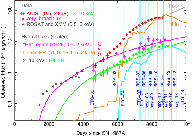
Figure 10: Comparing X-ray light curves with the hydrodynamic model fluxes. The H II region emission from the “no ER” model is shown by the curves beginning before day 3000 (magenta, green). The model does a reasonable job of matching the initial and late-time 3–10 keV flux (green diamonds) as well as modeling the initial 0.5–2 keV turn-on and growth (ROSAT points). At late-times the 0.5–2 keV flux from the H II region is in reasonable agreement with the measured very-broad flux (magenta diamonds), strengthening the identification of the v-b emission with the H II region. The emission from the shock collision with the dense ER rises steeply around day 6000 (orange, light blue). The light curve here (orange) is for the the “thin (or finite) ER” case of Figure 7; the gray line indicates the 0.5–2 keV flux when the ER continues in the “thick ER” case.

We use the hydrodynamic simulations as input to calculate the X-ray emission from each shocked mass-cut shell at each time step, employing the same scheme to track the NEI plasma state and carry out spectral calculations as outlined in Dwarkadas et al. (2010). Once the hydrodynamic solution is determined – fixing temperatures, ionization ages, and normalizations for the mass-cuts – the only free parameters are the abundances, an optional clumping set by a clumping fraction and its over-density, and the overall normalization set by the solid angle which each 1D model actually fills, $\Omega_{\mathrm{H\,II}}$ and $\Omega_{\rm ER}$. The abundances can be determined by fitting to the measured spectra, as described further in § 4.3 & 4.4. In terms of line broadening, the hydrodynamic velocities of the shells are used to include Doppler broadening in the synthesized spectra; in § 4.5 this “real” broadening is compared with the simple smoothing approximation that was used to quantify the v-b fraction (§ 2.4). Finally, for high shock velocities and low $\tau$’s, the simple $\propto\,v^{-2}$ behavior of $\beta=T_{e}/T_{i}$ (Ghavamian et al. 2007) produces $T_{e}$ values that are very low. As in Dwarkadas et al. (2010) we have used a modified $\beta(v)$ relation, suggested by the results of van Adelsberg et al. (2008), to set a minimum value of $\beta_{\rm min}\approx 0.06$.

Integrating the simulated spectra over the standard energy bands, 0.5–2 keV and 3–10 keV, we created model light curves, shown in Figure 10. The light curves for the two hydrodynamic simulations have been plotted separately and their (imagined) sum can reasonably describe the observed SN 1987A light curves over the full time span.

A filling fraction of $\Omega_{\mathrm{H\,II}}/4\pi=$ 0.26 is used to match the overall flux level for the H II (“no ER”) simulation, corresponding to emission from $\pm$ 15 degrees of the ring plane. This is roughly similar to other estimates of the H II region’s out-of-plane extent, e.g., by Michael et al. (2003, $\pm$ 30 degrees), Zhekov et al. (2010, $\pm$ 10 degrees), and Mattila et al. (2010, $\pm$ 7.2 degrees). The abundances for the H II light curve are set from fits to the early ACIS observation, described in § 4.3. One characteristic of this early-time H II emission is its relative hardness, e.g., for the deep ACIS-00 observation at day 5036 the ratio $F_{3-10}/F_{0.5-2}$ is 0.35 whereas at later times (day 7997, January 2009) the ratio has dropped to 0.12. As the light curves show, this is caused by the increase in the 0.5–2 keV flux due to the collision with the ER, rather than any decrease in the 3–10 keV emission.

In contrast to the H II region, the ER needs to produce emission primarily in the 0.5–2 keV range while keeping the 3–10 keV flux below the measured levels. Even though the ER is dense, our simulation still gives electron temperatures at/above 3 keV and thus relatively too much 3–10 keV flux. We could further increase the density of the ER, however given the resonable agreement of the slope of the “with ER” simulation (top panel of Figure 9) and the expectations of an inhomogeneous ER (e.g., the optical spots), we consider another, approximate approach. We can match the observed spectra by including emission from “clumps” in the ER with a density enhancement $\eta_{\rm clump}\approx\times$5.5 that fills $f_{\rm clump}\approx$ 30% of the CSM volume. The clumping is implemented at the spectral synthesis stage and introduces $kT_{e}\approx$ 0.5–0.8 keV emission components greatly enhancing the 0.5–2 keV emission (further details of the clumping implementation are given in § 4.4.) We acknowledge that for these clumping parameters most of the mass is in the very dense clumps (i.e., 0.30$\times$5.5 / (0.70$\times$1+0.30$\times$5.5)  $\approx$ 70%) and so the clumping is not a small perturbation on the ER hydrodynamics; therefore our 1D clumped ER simulation is just a placeholder for a realistic multi-dimensional simulation.

The single set of “with ER” light curves plotted in Figure 10 represents the bulk of the 0.5–2 keV flux increase; the fractional area used to scale the 1D model’s emission is very small: $\Omega_{\rm ER}/4\pi=$ 0.0016 . To put this into perspective, the fraction subtended by a uniform region with the dimensions of the optical ring, i.e., a region extending $\pm$ 0.05 arc seconds out of the plane at a radius of 0.83 arc seconds, is almost 40$\times$ larger, $\sim$ 0.0600. Hence, the small value indicates that the the ring is not uniformly dense and clumped, but rather it has “X-ray hot spots” analogous to the (still) discrete optical spots around the ring. Specifically, the 0.0016 value would arise from $\sim$ 20 regions each subtending a diameter of $\sim$ 2 degrees around the ring.

It is seen in Figure 10 that there is earlier-time flux growth above the H II emission that our plotted ER curve does not include. As mentioned in § 3.4, a range of inner radii is expected for the “ER” with some material at radii smaller than the 0.74 arc seconds where our modeled ER starts. Mentally “translating” our ER curve, we would expect to get flux beginning $\sim$ 5500 days by having a small fraction of ER material (perhaps 0.1 $\times$ $\Omega_{\rm ER}$) that is impacted at $\sim$ 4600 days. From our hydrodynamics this time corresponds to a radius of 4.8 $\times 10^{17}$ cm (0.155 pc) or 0.67 arc seconds. This radius is in reasonable agreement with the locations of the early optical spots (Sugerman et al. 2002, Figure 7).

4.3 H II Abundances from the Hydrodynamics

Using the set of shocked mass-cut shells at a given time-step of the hydrodynamics, we can create a spectral model in ISIS which is the sum of emission from each of the shells. The relative normalizations, temperatures, and ionizations ages for each model component (mass-cut shell) are set from the hydrodynamics. Tying the abundances of all components together, we then have a model which can be fit to measured spectra by adjusting the abundances and an overall normalization. By using the hydrodynamics to set the plasma properties we reduce the degeneracy in fitting that arises when the temperature(s) and ionization age(s) of the plasma are unconstrained and therefore we get accurate abundance values.

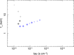
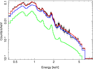
Figure 11: Left: The distribution of $kT_{e}$ and $\tau$ values in the H II hydrodynamics at the ACIS-00 epoch. Points of $(\tau,kT_{e})$ are plotted for all shocked mass shells in the model; symbols for the shocked ejecta (black) and CSM (blue) are larger/bold for brighter shells. Right: The ACIS-00 data (black) are fit with a model (red) that is the sum of the emission from the 14 shocked shells of the left panel; a single norm and the abundances of N, O, Ne, Mg, Si, S, and Fe were the only free parameters in the fit. The emission from the CSM shells (blue) is much larger than that of the shocked ejecta (green) at this early epoch.

Table 5: Degeneracy of H II Abundances when Fitting ACIS-00

	$kT$(s)	$\tau$(s)	—   Relative abundances     (1-$\sigma$ range)   —
Model	(keV)	($10^{11}$ s cm-3)	N	O	Ne	Si	Fe
1-shock	2.94–3.34	0.94–1.32	0.49–0.94	0.14–0.23	0.00–0.17	0.28–0.41	0.13–0.25
2-shock	0.22, 2.8	130, 1.4	0.34–0.72	0.11–0.17	0.27–0.35	0.29–0.38	0.083–0.12
Table 2	0.73, 4.2	11.6, 5.8	0.89–2.35	0.28–0.63	0.46–0.92	0.59–0.94	0.087–0.18
Hydro-noER	14 pairs in Figure 11		0.51–0.66	0.137–0.155	0.35–0.42	0.32–0.43	0.061–0.080

The early deep Chandra observation, ACIS-00, is the best data set to use to determine the abundances of the H II region (as opposed to the dense ER abundances, which may differ). These data also provide a useful example of how the fit abundances and their confidence ranges vary depending on the $kT$–$\tau$ model assumptions. The results of fitting four different cases are shown in Table 5. In all cases the redshifts and $N_{H}$ were frozen and the normalization(s) and abundances (N, O, Ne, Mg, Si, S, and Fe) were fit. In the first case a single vpshock component is fit giving $kT\approx 3.0$ keV and $\tau\approx$ 1.0$\times 10^{11}$ s cm^-3; these are similar to the values in Park et al. (2002). As a second case, we fit a 2-shock model fixing the temperatures, ionization ages, and $N_{H}$ based on values from Zhekov et al. (2010); this has a high temperature component similar to the 1-shock value along with a very low temperature component. In the third case, our model of Table 2 is shown, and because we have set $N_{\rm mid}$ to 0 for this early data it is also a 2-shock model with a different set of $kT$’s and $\tau$’s. Finally, we fit the data with the temperatures and ionization ages fixed based on the values from the “no ER” hydrodynamic model at the ACIS-00 epoch; these values are plotted in the left panel of Figure 11 and correspond to the model at the epoch shown in the top panel of Figure 8.

The reduced $\chi^{2}$ values are near 1.0 for all four of the fits, so they are equally acceptable from a data-fitting perspective. However, as the table shows, the 1-$\sigma$ ranges of the fit abundances depend very much on the $kT$–$\tau$ values used in the model. If it is possible to constrain the $kT$–$\tau$ values through other means or assumptions, as in the fourth case here, then the fit abundances will be both more realistic and better constrained. Hence, we adopt the hydrodynamics-based model as the most physical and include its abundances in the H II column of Table 6.

Table 6: Hydrodynamics-based Abundances and Others

	—  H II  —	—  ER  —	———  Other Abundances  ———
Parameters	ACIS-00	HETG- 07 & 11	Zhekov(‘09)	Zhekov(‘10)	Mattila(‘10)
N	0.584 $\pm$0.07	3.3 $\pm$1.2	0.56 ${}^{+{0.09}}_{-{0.06}}$	0.32 $\pm$0.04	2.5 $\pm$1.0
O	0.144 ${}^{+{0.011}}_{-{0.007}}$	0.382 $\pm$0.08	0.081 $\pm$0.01	0.07 $\pm$0.01	0.22 $\pm$0.04
Ne	0.381 $\pm$0.03	0.566 $\pm$0.03	0.29 $\pm$0.02	0.22 $\pm$0.01	0.69
Mg	0.270 $\pm$0.04	0.394 $\pm$0.02	0.28 ${}^{+{0.01}}_{-{0.02}}$	0.17 $\pm$0.01	$\cdots$
Si	0.373 $\pm$0.05	0.469 $\pm$0.02	0.33 ${}^{+{0.02}}_{-{0.01}}$	0.26 $\pm$0.01	$\cdots$
S	0.293 ${}^{+{0.12}}_{-{0.10}}$	0.556 $\pm$0.08	0.30 $\pm$0.06	0.36 $\pm$0.02	0.81 $\pm$0.4
Ar	0.00 ${}^{+{0.23}}_{-{0.0}}$	1.2 $\pm$0.5	[0.537]	[0.537]	0.47
Fe	0.070 ${}^{+{0.010}}_{-{0.009}}$	0.225 $\pm$0.02	0.19 ${}^{+{0.02}}_{-{0.00}}$	0.10 $\pm$0.01	0.20 $\pm$0.1
$f_{clump}$	$\cdots$	0.30 $\pm$0.02	$\cdots$	$\cdots$	$\cdots$
$\eta_{clump}$	$\cdots$	5.51 $\pm$0.45	$\cdots$	$\cdots$	$\cdots$

Note. — Abundances are relative to the solar photospheric values of Anders & Grevesse (1989), AG89. Values in brackets were fixed; those not tabulated were set to: H=1, He=2.57, C=0.03, Ar=0.03, Ca=0.03, and Ni=0.07. $N_{H}$ has been fixed at 1.3$\times 10^{21}$ cm^-2.

4.4 ER Abundances and Clumping

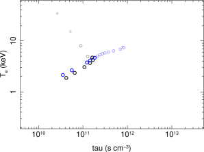
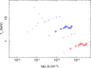
Figure 12: Distributions of $kT_{e}$–$\tau$ for the hydrodynamics at the HETG-11 epoch. Points of $(\tau,kT_{e})$ are plotted for all shocked mass shells in the H II (no-ER, left panel) and “with ER” (right panel) simulations. Symbols for the shocked ejecta (black) and CSM (blue) are larger/bold for brighter shells. The H II distribution is similar to earlier times (Figure 11, left panel) although shifted to somewhat higher $\tau$ and $kT_{e}$ values. The “with ER” distribution (right panel) is dominated by components at much higher $\tau$ values; the addition of a clumped component introduces additional $kT_{e}$–$\tau$ values (red) that are scaled from the non-clumped CSM values.

We can similarly fit hydrodynamics-based models to the later observations where the emission is dominated by the shocked ER material and in this way determine the ER abundances. At these times there will still be a contribution from the H II region, i.e., the v-b component. This contribution is removed from the data before fitting by evaluating our “no ER” model at the appropriate epoch and subtracting the predicted counts from the data before proceeding with ER-model fitting.

The $kT_{e}$–$\tau$ values of the shocked mass-cuts in our H II and ER models at the HETG-11 epoch are shown in Figure 12. As the blue points in the “with ER” (right) panel show, the $kT_{e}$ values in the shocked dense ring are mostly at/above 3 keV. Given these temperatures, simply adjusting the abundances is insufficient to fit the data, there is simply too little low-$kT_{e}$, high-$\tau$ plasma. We have therefore included “clumps” in the ER material following the scheme in Dwarkadas et al. (2010).

For each of the shocked CSM mass-cuts (blue circles in the right panel of Figure 12) we add an additional model component with its temperature reduced by the clump’s density enhancement, $kT_{e}^{\prime}=kT_{e}/\eta_{\rm clump}$, and its ionization age increased to $\tau^{\prime}=\eta_{\rm clump}\,\tau$. The additional clumped components are shown as red circles in the right panel of Figure 12 for $\eta_{\rm clump}\approx$ 5.5. The original and clumped components have additional factors in their norms of $(1-f_{\rm clump})$ and $f_{\rm clump}\,\eta_{\rm clump}^{2}$, respectively, where $f_{\rm clump}\approx$ 30% is the volume fraction of clumped material. The resulting ISIS fit function at the HETG-11 epoch consists of 45 NEI model components but with only 9 free parameters: an overall normalization, the 2 clumping parameters, and the ER abundances of O, Ne, Mg, Si, S, and Fe.

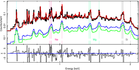
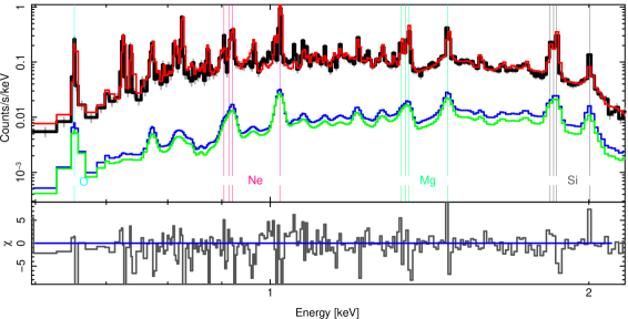
Figure 13: HETG(MEG) spectra and full hydrodynamics-based models. The HETG-07 (top) and HETG-11 (bottom) data (black) are reasonably fit by the total (H II plus nominal clumped-ER) model spectra (red). The H II-shocked-CSM (blue) and the H II-shocked-ejecta (green) components are also shown individually. Note the relative growth of the shocked ejecta (green) between the epochs; hence at late times the ejecta and its abundances will dominate the H II (i.e., v-b) component.

We fit both the deep HETG-07 and HETG-11 data sets with their appropriate-epoch hydrodynamics-based models, determining the abundances and clumping parameters for each. There are only small differences between the 2007 and 2011 fits, so we have adopted nominal ER parameters that are the average values given in the “ER” column of Table 6. Note that the N abundance was set based on similar fitting to the RGS-11 spectrum. These values were then used to generate our light curve (§ 4.2) and to fit the hydrodynamics-based models to all of the grating spectra with only a single normalization adjustment. As examples, Figure 13 compares the two deep HETG spectra with the sum of the hydrodynamics-based emission from the H II region and the nominal-parameter ER emission.

Given our crude clumping implementation and the system’s physical complexity, we have less confidence in the accuracy, i.e., agreement with reality, of our ER abundances than those we determined for the H II region at the ACIS-00 epoch. However since the ER $kT$s and $\tau$s are based on a hydrodynamic solution there is some expectation that they will be an improvement over simpler multi-shock models. For comparison, we’ve also included in Table 6 the abundances given by Zhekov et al. (2009, multi-shock fits to grating data), Zhekov et al. (2010, RSS fits to the ACIS data), and Mattila et al. (2010, optical & NIR data before the ER collision). Our ER abundances for N, O, Ne, and S do appear to be in someshat better agreement with the Mattila et al. (2010) values than are the other X-ray-determined abundances.

This is a good place to compare the free parameters of the Zhekov et al. (2010) model (Z10 in the following) with ours, in terms of their number and their values. The two model geometries are similar at later times, both are dominated by the ER emission, Figure 6, and both make approximations to include clumped ER material. Each model fixes time-independent values for the CSM’s $\rho(r)$, the $N_{H}$, and the abundances. In addition to these, Z10 fit six parameters for each observation: the values of the temperature, ionization age, and emission measure for both the blast wave (BW) and the transmitted shock (TS). For example, for their latest data point which is near the HETG-07 epoch, the values for these are: $kT_{\rm BW}\approx$ 1.7 keV, $kT_{\rm TS}\approx$ 0.33 keV, $\tau_{\rm BW}\approx$ 1.4$\times 10^{11}$ s cm^-3, $\tau_{\rm BW}\approx$ 30$\times 10^{11}$ s cm^-3, and the respective emission measures are 1.05 and 9.5 in units of 10⁵⁹ cm^-3. In contrast, all of our mass-shell $kT$ and $\tau$ values are fixed by the hydrodynamics, e.g., as for HETG-11 in Figure 12, and our ER modeling adds only three further time-independent parameters: the overall normalization, $\Omega_{\rm ER}$, and the two clumping parameters. In our approximation the clump over-density, $\eta_{\rm clump}\approx 5.5$, sets the ratio of ER-to-clump temperature. For the Z10 values above, this ratio is $T_{\rm BW}/T_{\rm TS}\approx 5$, close to ours. Likewise, the Z10 emission measure ratio, ${\rm EM}_{\rm TS}/{\rm EM}_{\rm BW}\approx 9$, is in the ball park of our value which is given by $f_{\rm clump}\eta_{\rm clump}^{2}/(1-f_{\rm clump})\approx 13$, using our clump volume fraction $f_{\rm clump}\approx 30$ %. In constrast, the clump volume fraction for the Z10 model is of order 5 % because the clump-to-ambient density ratio is large: $\rho_{\rm TS}/\rho_{\rm BW}\approx 14$; this latter value is a function of the temperature ratio as shown in a plot in the Appendix of Zhekov et al. (2009). These comparisons suggest that there may be some degeneracy between over-density and volume fraction for the clumps. In anycase, it is clear that both approaches here are only approximating the complex 2D/3D density structures of the real ER.

4.5 Very-Broad Spectrum from the Simulation

We can check our decision to use a smoothed version of the spectrum as the model for the v-b component by directly comparing the two of them, as shown in Figure 14. Here, the broad lines in the “real” (from the hydrodynamics) v-b component are similar to those in the smoothed version of the 3-shock fit to the data. This similarity can be roughly explained using the $kT_{e}$–$\tau$ distributions shown in Figure 12: the H II (v-b) emission is dominated by components with $kT_{e}\approx$ 2.5 keV and $\tau\approx$ 6$\times 10^{10}$ s cm^-3, whereas the main ER emission is from clumped material with $kT_{e}\approx$ 0.7 keV and $\tau\approx$ 2$\times 10^{13}$ s cm^-3. Putting these values into a vnei model gives similar line structures for the two cases, hence, the high-$kT$-low-$\tau$ plasma produces ionization states and emission lines that are similar to those of a low-$kT$-high-$\tau$ plasma. Based on this comparison we did, however, decide to ignore the Fe XVII range 0.70–0.75 keV when doing the v-b fitting as these lines were clearly not present in the hydrodynamic-based v-b spectrum.

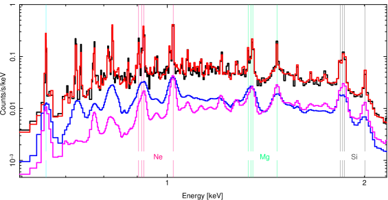
Figure 14: Comparing the heuristic very-broad spectrum with the hydrodynamics-based H II v-b spectrum. The HETG-07 data (black) are shown with the best-fit 3-shock model (red) that includes a v-b component (blue). This “smoothed version of the model” form of the v-b component is compared with the multi-shells model spectrum at the HETG-07 epoch (magenta). Ignoring the overall continuum shape, they are in reasonable line-broadening agreement except for the lack of significant Fe XVII lines between 0.70–0.75 keV in the hydro-based model.

In terms of the assumption of a constant width of the v-b emission in time (the evolution path shown in Figure 4), the average bulk motion of the shocked H II material in the “no ER” simulation varies (only) from 4200 km s^-1 to 3850 km s^-1 from the HETG-99 epoch to an age of over 25 years (9000+ days). This is also seen in the locations of the “no ER” CD and FS locations, lower-left panel of Figure 9, which follow nearly straight lines with overall slopes of 4300 km s^-1 and 5100 km s^-1, respectively.

4.6 The Mass of the X-Ray Emitting Material

We can calculate the shocked mass for different components and epochs of the model. For the H II region, at the ACIS-00 epoch the FS is at $\sim$ 0.162 pc (top panel of Figure 8) and the mass of shocked CSM in the simulation, correcting for the opening angle normalization $\Omega_{\mathrm{H\,II}}/4\pi\approx$ 0.26 (§ 4.2), is 0.012 solar masses. At this time our model shows $\sim$ 0.005 solar masses of ejecta are shocked within the same opening angle. Later, at the HETG-11 epoch, the shocked H II material that produces the v-b emission in our model has grown to 0.042 solar masses along with an additional 0.024 solar masses of shocked ejecta. Our H II mass values compare in order of magnitude with the mass of 0.018 solar masses that Mattila et al. (2010) require in their low-density (10² atoms cm^-3) H II component.

The total “4$\pi$” mass of the thin ER is 1.18 solar masses; however, correcting for the small solid-angle fraction, $\Omega_{\rm ER}/4\pi\,\approx\,0.0016$, we get only $\sim$ 0.0019 solar masses of ER that are shocked at the HETG-11 epoch (when the FS is exiting the thin ER). Including the extra mass due to clumping (multiplying by a factor of 2.35, § 4.2), we have 0.0045 solar masses as the total shocked-ER mass that produces the observed non-v-b X-rays in our model at the HETG-11 epoch. This is to be compared with an estimate of the total mass of the UV-ionized ER of 0.058 solar masses distributed among three densities of 1.4$\times 10^{3}$, 4.2$\times 10^{3}$, and 4.2$\times 10^{4}$ amu cm^-3 (Mattila et al. 2010, using $\sim$ 1.4 amu per atom); of this total, 0.0120 solar masses are in the highest-density component, almost 3 times our X-ray inferred mass. However, it could well be that our ER X-ray emission is a factor of a few overly efficient per mass and including this as an error bar puts us in a gray area in trying to use this mass comparison to decide if all of the ionization-visible dense ER has been shocked at the current $\sim$ 25 year age of SN 1987A.

4.7 Image Implications

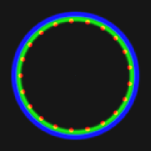
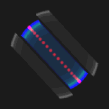
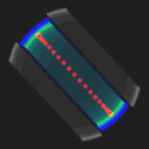
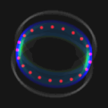
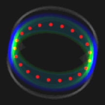
Figure 15: Hydrodynamics-based geometric emission models of SN 1987A at epochs 2004.5 (left column) and 2011.5 (right column). Three views are shown: a “polar” view (top; looking perpendicular to the equatorial plane), a “side” view (middle; north is up and the Earth is to the left), and the usual sky view (bottom; north up, east to left). Four emission components are color-coded: the shocked H II material (blue), the reverse-shocked ejecta (green), the emission from the shocked ER (red spots), and higher-lattitude 8.6 GHz radio emission (gray).

We can construct schematic geometric visualizations of SN 1987A using our simple hydrodynamic models to set the locations and fluxes of the components at a given epoch. The main emission components at two different epochs are shown in multiple views in Figure 15 using a color-coding similar to that for the shocked plasma in the schematic of Figure 6. These images were created using simple software extensions to ISIS (Dewey & Noble 2009) .

The H II (“no ER”) simulation gives rise to emission from i) shocked H II material and ii) reverse-shocked ejecta; these regions extend out of the ER plane as shown in the images. The “with ER” simulation is shown using a schematic geometry of 21 discrete spots to emphasize our “X-ray hot spots” conclusion that is based on the small value of $\Omega_{\rm ER}$. The “with ER” emission components include: iii) the shocked dense ER and its clumps, iv) the shocked H II material that is in the plane of the ER, and v) reverse-shocked ejecta also in the ER plane. Because the effective solid angle associated with the ER simulation is so small ($\Omega_{\rm ER}/4\pi=$ 0.0016) these last two components make only minor flux contributions which are exceeded by the first three. We note that component “iv)” is the plasma that is “shocked again” in the reflected shock structure (RSS) paradigm (Zhekov et al. 2009, 2010); our “with ER” hydrodynamics does show the reflected shock(s) having velocity effects on the shocked H II region interior to the shocked ER for about 1.5 years, after which the region’s velocity recovers and is similar to other regions, e.g., see the velocity curve in Figure 8, bottom panel.

These visualizations suggest the need for fitting the X-ray imaging data with multiple spatial components and provide some guidance on the component properties. Recent work of Ng et al. (2009) has explored a two-component spatial model in fitting SN 1987A’s image, and as they emphasize, further observations are needed to come to a firm conclusion.

5 CONCLUSIONS

In this paper we have modelled the X-ray emission from SN 1987A, focussing on the very-broad (v-b) component seen with the high-resolution grating instruments. Although the CSM of SN 1987A is known to have a complex shape from optical observations, we have chosen to model it using 1D simulations in and out of the equatorial plane, our H II and ER hydrodynamics. Even with these simplifying assumptions the models yield a good fit to the X-ray-measured radii and growth rates, the multi-band X-ray light curves, and the high-resolution X-ray spectra.

Our results show that better fits to the X-ray spectra over the last decade are obtained if a very-broad component of emission, with a FWHM of about 9300 km s^-1, is included. Such a v-b component is present in the data over at least the last decade. Our hydrodynamic simulations provide a natural explanation for this component: it arises from the shocked H II material and it is the dominant X-ray component until $\sim$ 5500 days after the SN explosion. Since then the total 0.5–2 keV flux dramatically increased due to the “ER” collision, yet the inferred 0.5–2 keV flux of the v-b component itself continued to grow in agreement with our hydrodynamics expectations. Identifying the 3–10 keV flux as originating primarilly from the v-b component provides a natural explanation for the difference in the 0.5–2 and 3–10 keV light curves. At the present epoch, the v-b contribution is $\sim$ 20% of the total 0.5–2 keV flux, and of this the hydrodynamics suggests that roughly half is coming from reverse-shocked ejecta. This ejecta contribution should grow and may cause the v-b component to become selectively enhanced in lines that reflect the (outer) ejecta composition.

Our ER hydrodynamics adquately reproduces the observed X-ray image radii and the bulk of the late-time 0.5–2 keV flux increase. We do require clumps in the ER with density enhancements of $5.5\times$ the $\sim$ 10⁴ amu cm^-3 ambient ER values, not unlike the clumps that Zhekov et al. (2010) have added within their smooth CSM density profile. These are approximations to the actual 2D/3D density structure of the shock-ER interaction; it would not be surprising if the effective clumping parameters might change in time, e.g., as clumps evaporate and/or turbulent structures evolve.

Our approach allows us to make predictions of what the image size, X-ray spectrum and light curve will look like in the next few years, in particular for the two cases of i) a continuing on-going interaction with dense ER material (our “thick ER” case) and ii) the drop in flux if the ER is “thin”. In this latter case, the FS in the equatorial plane has generally exited the densest parts of the ER and has begun moving into lower-density material as suggested by Park et al. (2011). For this case our hydrodynamics shows a decrease in the 0.5–2 keV flux of $\sim$ 17 % per year. Note that a third option that cannot be completely ruled out is that the FS will encounter larger amounts of dense ER material, e.g., the main body of the ER; this would result in even greater increases in flux than we have shown here. Comparing these and more realistic multi-dimensional predictions with future observations will provide significant information regarding the thickness, density, and structure of the equatorial ring and the H II region within and outside the equatorial plane as SN 1987A moves into a new phase.

Appendix A Spectral Models and the gsmooth Function

The 3-shock model used in § 2.3 makes use of the XSPEC spectral library and is defined in ISIS with the command:

$${\tt fit\_fun(~{}"phabs(1)*gsmooth(1,\,vpshock(1)+vpshock(2)+vpshock(3)\,)"~{});}$$ (A1)

where the trailing “;” is the S-Lang end-of-expression character. The gsmooth(1) function here is used to add blur to the model in order to account for spatial and spectral effects that are unique to SN 1987A; the gsmooth parameters Sig@6keV and Index and their values for this purpose are described further below.

A similar expression is used to define the v-b 3-shock model used in § 2.4 as the sum of the original 3-shock model and a very-broad version of itself:

$${\tt fit\_fun(~{}~{}"setvb(1)*phabs(1)*"~{}~{}+}$$ (A2)

$$~{}~{}{\tt"(~{}(1-fracbroad)*gsmooth(1,vpshock(1)+vpshock(2)+vpshock(3))+"~{}~{}+}$$

$$~{}~{}~{}~{}~{}~{}~{}~{}~{}~{}{\tt"fracbroad*gsmooth(2,vpshock(1)+vpshock(2)+vpshock(3))~{})"~{}~{}~{});}$$

Here the S-Lang variable, fracbroad, sets the fraction of the total which is in the v-b component and the second gsmooth term sets the width of the v-b emission. For a v-b component having a FWHM of $v_{\mathrm{v}\textrm{\footnotesize-}\mathrm{b}}$, the Sig@6keV parameter is set to $6v_{\mathrm{v}\textrm{\footnotesize-}\mathrm{b}}/(2.35c)$ and the Index parameter is set to 1, as discussed further below. The model component (setvb) is a dummy function which returns unity in the spectral model but is used to control the broad-fraction variable from an ISIS fit parameter, setvb(1).fb. This is accomplished before the model is defined with a few lines of code:

public variable fracbroad;
% Define a dummy model function to set the broad fraction
define setvb_fit (l,h,p)
{
% set fracbroad from the input parameter:
fracbroad = p[0];
return 1;
}
add_slang_function ("setvb", ["fb"]);

In the remainder of this section we provide more specifics on the gsmooth function and its parameters.

Table 7: Spatial-Spectral Blur Parameters

	$\sigma_{\rm O\,VIII}$	$\sigma_{\rm Mg}$		$\sigma_{6}$, Sig@6keV
Grating	(eV)	(eV)	$\alpha$, Index	(keV)
RGS	0.628	[1.36]	1.0000	0.00580
HETG	0.881	2.14	1.1454	0.01124
LETG	1.893	5.90	1.4682	0.04946

The gsmooth function convolves a spectral model with a Gaussian function whose width, $\sigma_{E}$, varies with energy according to:

$$\sigma_{E}=\sigma_{6}~{}(E_{\rm keV}/6.0)^{\alpha}~{}.$$ (A3)

The constants of this equation, $\sigma_{6}$ and $\alpha$, are set through the values of the gsmooth parameters Sig@6keV and Index, respectively. This versatile function can be used to approximate instrumental effects in place of an rmf. For the case of $\alpha=0$ it produces a constant-with-energy blur, e.g., simulating a micro-calorimeter-like response. The case of $\alpha=0.5$ gives a resolution, $dE_{\rm FWHM}$, that goes as the square-root-of-energy, e.g., as in a proportional-counter or a CCD detector. For $\alpha=1$ the resolving-power, $E/dE_{\rm FWHM}$, is constant, and for $\alpha=2$ we have the case of a blur that is constant in wavelength as is nearly the case for a grating instrument like the HETG.

The smoothing term can also be used to include additional source spectral properties, for example, the Doppler blur from a Gaussian velocity spread, $v_{\rm rms}$, is obtained by setting $\alpha=1$ and $\sigma_{6}=6\,v_{\rm rms}/c$ ; if the FWHM velocity width is given, then we have $\sigma_{6}=6\,v_{\rm FWHM}/(2.35c)$. It is in exactly this way that we use gsmooth(2) in Expression A2 to produce the v-b component in our model.

Finally, we also make use of the gsmooth function to account for additional blurs that are present in the narrow lines of the SN 1987A grating spectra but are not included in the spectral model (vpshock) nor in the point-source instrumental responses (rmfs). These blurs have been noted and included in previous grating-data analyses (Zhekov et al. 2005; Dewey et al. 2008; Sturm et al. 2010) and result from i) bulk and turbulent motion of the X-ray emitting plasma and ii) spatial-spectral effects which broaden the observed line widths due to the spatial size of SN 1987A. In the context of the gsmooth function the former is accounted for with an $\alpha=1$ behavior and the latter with an $\alpha=2$ dependence. The combination of both effects can be approximated using an intermediate value of $\alpha$ determined by measuring the narrow-component line width at two energies. For the analyses here this has been done using regions including the O VIII line and the Mg line (1.28 – 1.55 keV); the measured values and resulting gsmooth parameters are given in Table 7. Note that the RGS has $\alpha=1$ because SN 1987A is spatially unresolved by XMM-Newton.

References

- Anders & Grevesse (1989) Anders, E., & Grevesse, N. 1989, Geochim. Cosmochim. Acta, 53, 197
- Borkowski et al. (1997a) Borkowski, K. J., Blondin, J. M., & McCray, R. 1997a, ApJ, 476, L31
- Borkowski et al. (1997b) —. 1997b, ApJ, 477, 281
- Borkowski et al. (2001) Borkowski, K. J., Lyerly, W. J., & Reynolds, S. P. 2001, ApJ, 548, 820
- Canizares et al. (2000) Canizares, C. R., et al. 2000, ApJ, 539, L41
- Canizares et al. (2005) —. 2005, PASP, 117, 1144
- Chevalier (1982) Chevalier, R. A. 1982, ApJ, 258, 790
- Chevalier (1992) —. 1992, Nature, 355, 617
- Chevalier & Dwarkadas (1995) Chevalier, R. A., & Dwarkadas, V. V. 1995, ApJ, 452, L45
- Chevalier & Liang (1989) Chevalier, R. A., & Liang, E. P. 1989, ApJ, 344, 332
- Colella & Woodward (1984) Colella, P., & Woodward, P. R. 1984, Journal of Computational Physics, 54, 174
- den Herder et al. (2001) den Herder, J. W., et al. 2001, A&A, 365, L7
- Dewey & Noble (2009) Dewey, D., & Noble, M. S. 2009, in Astronomical Society of the Pacific Conference Series, Vol. 411, Astronomical Data Analysis Software and Systems XVIII, ed. D. A. Bohlender, D. Durand, & P. Dowler, 234–238
- Dewey et al. (2008) Dewey, D., Zhekov, S. A., McCray, R., & Canizares, C. R. 2008, ApJ, 676, L131
- Dwarkadas (2007a) Dwarkadas, V. V. 2007a, in Revista Mexicana de Astronomia y Astrofisica Conference Series, Vol. 30, Revista Mexicana de Astronomia y Astrofisica Conference Series, 49–56
- Dwarkadas (2007b) Dwarkadas, V. V. 2007b, in American Institute of Physics Conference Series, Vol. 937, Supernova 1987A: 20 Years After: Supernovae and Gamma-Ray Bursters, ed. S. Immler, K. Weiler, & R. McCray, 120–124
- Dwarkadas et al. (2010) Dwarkadas, V. V., Dewey, D., & Bauer, F. 2010, MNRAS, 407, 812
- Dwarkadas & Gruszko (2012) Dwarkadas, V. V., & Gruszko, J. 2012, MNRAS, 419, 1515
- Gaensler et al. (1997) Gaensler, B. M., Manchester, R. N., Staveley-Smith, L., Tzioumis, A. K., Reynolds, J. E., & Kesteven, M. J. 1997, ApJ, 479, 845
- Ghavamian et al. (2007) Ghavamian, P., Laming, J. M., & Rakowski, C. E. 2007, ApJ, 654, L69
- Haberl et al. (2006) Haberl, F., Geppert, U., Aschenbach, B., & Hasinger, G. 2006, A&A, 460, 811
- Hasinger et al. (1996) Hasinger, G., Aschenbach, B., & Truemper, J. 1996, A&A, 312, L9
- Houck & Denicola (2000) Houck, J. C., & Denicola, L. A. 2000, in Astronomical Society of the Pacific Conference Series, Vol. 216, Astronomical Data Analysis Software and Systems IX, ed. N. Manset, C. Veillet, & D. Crabtree, 591
- Huenemoerder et al. (2011) Huenemoerder, D. P., et al. 2011, AJ, 141, 129
- Inoue et al. (1991) Inoue, H., Hayashida, K., Itoh, M., Kondo, H., Mitsuda, K., Takeshima, T., Yoshida, K., & Tanaka, Y. 1991, PASJ, 43, 213
- Itoh et al. (1987) Itoh, H., Hayakawa, S., Masai, K., & Nomoto, K. 1987, PASJ, 39, 529
- Larsson et al. (2011) Larsson, J., et al. 2011, Nature, 474, 484
- Lundqvist (1999) Lundqvist, P. 1999, ApJ, 511, 389
- Luo & McCray (1991a) Luo, D., & McCray, R. 1991a, ApJ, 372, 194
- Luo & McCray (1991b) —. 1991b, ApJ, 379, 659
- Luo et al. (1994) Luo, D., McCray, R., & Slavin, J. 1994, ApJ, 430, 264
- Masai et al. (1991) Masai, K., Itoh, H., & Nomoto, K. 1991, in European Southern Observatory Conference and Workshop Proceedings, Vol. 37, European Southern Observatory Conference and Workshop Proceedings, ed. I. J. Danziger & K. Kjaer, 197
- Masai & Nomoto (1994) Masai, K., & Nomoto, K. 1994, ApJ, 424, 924
- Mattila et al. (2010) Mattila, S., Lundqvist, P., Gröningsson, P., Meikle, P., Stathakis, R., Fransson, C., & Cannon, R. 2010, ApJ, 717, 1140
- McCray (2007) McCray, R. 2007, in American Institute of Physics Conference Series, Vol. 937, Supernova 1987A: 20 Years After: Supernovae and Gamma-Ray Bursters, ed. S. Immler, K. Weiler, & R. McCray, 3–14
- Michael et al. (2002) Michael, E., et al. 2002, ApJ, 574, 166
- Michael et al. (2003) —. 2003, ApJ, 593, 809
- Ng et al. (2009) Ng, C.-Y., Gaensler, B. M., Murray, S. S., Slane, P. O., Park, S., Staveley-Smith, L., Manchester, R. N., & Burrows, D. N. 2009, ApJ, 706, L100
- Ng et al. (2008) Ng, C.-Y., Gaensler, B. M., Staveley-Smith, L., Manchester, R. N., Kesteven, M. J., Ball, L., & Tzioumis, A. K. 2008, ApJ, 684, 481
- Panagia (1999) Panagia, N. 1999, in IAU Symposium, Vol. 190, New Views of the Magellanic Clouds, ed. Y.-H. Chu, N. Suntzeff, J. Hesser, & D. Bohlender, 549
- Park et al. (2002) Park, S., Burrows, D. N., Garmire, G. P., Nousek, J. A., McCray, R., Michael, E., & Zhekov, S. 2002, ApJ, 567, 314
- Park et al. (2004) Park, S., Zhekov, S. A., Burrows, D. N., Garmire, G. P., & McCray, R. 2004, ApJ, 610, 275
- Park et al. (2006) Park, S., Zhekov, S. A., Burrows, D. N., Garmire, G. P., Racusin, J. L., & McCray, R. 2006, ApJ, 646, 1001
- Park et al. (2005) Park, S., Zhekov, S. A., Burrows, D. N., & McCray, R. 2005, ApJ, 634, L73
- Park et al. (2011) Park, S., Zhekov, S. A., Burrows, D. N., Racusin, J. L., Dewey, D., & McCray, R. 2011, ApJ, 733, L35
- Potter et al. (2009) Potter, T. M., et al. 2009, ApJ, 705, 261
- Racusin et al. (2009) Racusin, J. L., Park, S., Zhekov, S., Burrows, D. N., Garmire, G. P., & McCray, R. 2009, ApJ, 703, 1752
- Sturm et al. (2010) Sturm, R., Haberl, F., Aschenbach, B., & Hasinger, G. 2010, A&A, 515, A5
- Sugerman et al. (2002) Sugerman, B. E. K., Lawrence, S. S., Crotts, A. P. S., Bouchet, P., & Heathcote, S. R. 2002, ApJ, 572, 209
- Suzuki et al. (1993) Suzuki, T., Shigeyama, T., & Nomoto, K. 1993, A&A, 274, 883
- van Adelsberg et al. (2008) van Adelsberg, M., Heng, K., McCray, R., & Raymond, J. C. 2008, ApJ, 689, 1089
- Zhekov et al. (2005) Zhekov, S. A., McCray, R., Borkowski, K. J., Burrows, D. N., & Park, S. 2005, ApJ, 628, L127
- Zhekov et al. (2006) —. 2006, ApJ, 645, 293
- Zhekov et al. (2009) Zhekov, S. A., McCray, R., Dewey, D., Canizares, C. R., Borkowski, K. J., Burrows, D. N., & Park, S. 2009, ApJ, 692, 1190
- Zhekov et al. (2010) Zhekov, S. A., Park, S., McCray, R., Racusin, J. L., & Burrows, D. N. 2010, MNRAS, 407, 1157