Impact of individual nodes in Boolean network dynamics

Abstract

Boolean networks serve as discrete models of regulation and signaling in biological cells. Identifying the key controllers of such processes is important for their understanding and planning further analysis. We quantify the dynamical impact of a node as the probability of damage spreading after switching the node’s state. The leading eigenvector of the adjacency matrix is a good predictor of dynamical impact in case of long-term spreading. Quality of prediction is further improved when eigenvector centrality is based on the weighted matrix of activities rather than the unweighted adjacency matrix. Simulations are performed with random Boolean networks and a model of signaling in fibroblasts. The findings are supported by analytic arguments from a linear approximation of damage spreading.

1 Introduction

Boolean networks are coarse-grained models of the regulatory dynamics that controls the survival and proliferation of a living cell [1, 2, 3, 4]. The dynamics is time- and state-discrete. This Boolean abstraction assumes that small differences in concentration levels are irrelevant. The binary distinction of a low or a high concentration of each bio-molecule is sufficient to capture the dynamics.

A purely theoretical branch of studies is devoted to randomly constructed Boolean networks [5, 6] and strives to elucidate generic features of Boolean dynamics. From the perspective of statistical mechanics, averaged macroscopic quantities in the limit of large system size are described in dependence of ensemble parameters such as the probability distribution of the employed Boolean functions [7, 8] and the degree distributions of the networks [9, 10]. The number of attractors (ergodic subsets of the state space) [2, 11, 12, 13] and the stability under perturbations [14, 9, 15, 16, 17, 18, 19, 20] have been investigated. The underlying fundamental result is a transition between convergent (stable) and divergent (unstable) dynamics when the input sensitivity of the Boolean functions passes a critical value [14, 21].

In recent years, the theory of random ensembles has been complemented by case studies showing that suitably constructed Boolean networks capture the behaviour of empirical regulatory systems [22, 23, 24, 25, 26]. These system-specific Boolean networks are obtained by compiling biochemical interactions from the literature [27], by discretizing existing models of differential equations [28], or by inference from data by a dedicated algorithm [29].

With the advent of system-specific Boolean models, new conceptual questions and analytical and numerical challenges arise. In particular, the response of the system to external intervention may be quantified in a more detailed manner than an averaging over all eligible perturbations. Since each node now represents a specific biochemical entity, a node’s individual impact on the dynamics is of interest. The prediction of nodes’ impacts from the model may be compared to biological experiments. It is expected to trigger additional experiments and lead to improvement of models.

The goal of this contribution is to establish a formal notion of node impact in Boolean dynamics and its relation to a node’s topological position in the network. We perform a linear approximation of the long-term effect of a perturbation at a specific node $i$. We find that, in good approximation, the expected impact is monotonically related to the entry of $i$ in the leading eigenvector of the adjacency matrix. When not only the network structure but also the Boolean functions are known, the estimate is improved by replacing the adjacency matrix with a weighted matrix of the activity values derived from the functions. The analytic approximations are validated by numerical studies of random Boolean networks and an empirical network from the literature.

2 Boolean networks

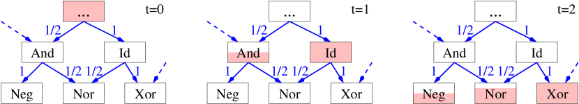
Figure 1: Probabilistic description of damage spreading in a Boolean network. The estimated damage probability $p_{i}(t)$ for a node $i$ at time $t$ is indicated by the height of the shaded area. At time $t=0$, the upper node is perturbed, thus having a damage probability 1. Neglecting correlations, the probability that a damage spreads from a node $i$ to a node $j$ is the activity $\alpha_{ij}$ as a label on each connection $i\rightarrow j$. Note that the case of more than one perturbed input, such as for the node with the Nor-function, is not captured by the activities. In the analytic treatment, we assume linear superposition of damage probabilities. The node performing Nor has an estimated damage probability $(1/2)(1/2)+1(1/2)=3/4$ at time $t=2$.

A Boolean network is a state- and time-discrete dynamical system. The dynamics is defined by an iteration

$$x(t+1)=f(x(t))$$ (1)

with $N$ Boolean dynamical variables written as a binary vector $x(t)\in\{0,1\}^{N}$ at each time $t\in\mathbb{N}\cup\{0\}$. The mapping $f:\{0,1\}^{N}\rightarrow\{0,1\}^{N}$ is typically sparse: calculating the state $x_{j}(t+1)$ requires knowledge of the state $x_{i}(t)$ for a few ($\ll N$) indices $i$ at the previous time step. When the system is pictured as a directed network, the nodes $\{1,2,\dots,N\}$ carry the dynamic variables $x_{1},x_{2},\dots,x_{N}$ interacting along a relatively small number of directed arcs. Subindices address components of a vector such that $x_{j}$ is the Boolean state of node $j$ and $f_{j}$ is its Boolean function.

In order to formalize and quantify these ideas, we consider the $x_{i}$-dependence of $f$ as the mapping

$$\partial^{(i)}f_{j}(x)=\left\{\begin{array}[]{cl}1&\textrm{if }f_{j}(x)\neq f_{j}(x^{\updownarrow i})\\ 0&\textrm{otherwise}\end{array}\right.$$ (2)

This is the Boolean analogue of the usual partial derivative of a function, using $x^{\updownarrow i}$ to denote state vector $x$ with its $i$-th entry negated. Note that $\partial^{(i)}f$ also maps from $\{0,1\}^{N}$ to $\{0,1\}^{N}$. By averaging $\partial^{(i)}f$ over all states with equal weight, the activity of $i$ on $j$ is obtained as

$$\alpha_{ij}(f)=2^{-N}\sum_{x\in\{0,1\}^{N}}\partial^{(i)}f_{j}(x)$$ (3)

The activity $\alpha_{ij}(f)$ is the probability that a perturbation (negation of state) at node $i$ causes a perturbation at node $j$ in the subsequent time step, assuming that all $2^{N}$ state vectors occur with equal probability. The sensitivity of the Boolean function $f_{i}$ is the sum of its incoming activities,

$$s_{i}(f)=\sum_{j=1}^{N}\alpha_{ji}~{}.$$ (4)

Likewise, we define the strength of $f_{i}$ as the sum of outgoing activities

$$\sigma_{i}(f)=\sum_{j=1}^{N}\alpha_{ij}~{}.$$ (5)

The directed network on the nodes $\{1,2,\dots,N\}$ obtained from $f$ contains an arc from node $i$ to node $j$ if and only if $\alpha_{ij}(f)\neq 0$. The adjacency matrix $A$ of the network has an entry $a_{ij}=1$ if $\alpha_{ij}(f)\neq 0$ and $a_{ij}=0$ otherwise.

3 Dynamical impact

So far we have considered the average effect of a flip perturbation at the input $i$ of a Boolean function $f_{j}$ on the output. Now we ask about the long-term behaviour of the whole system after a perturbation. We define

$$H_{i}(t)=\{x\in\{0,1\}^{N}:f^{t}(x)\neq f^{t}(x^{\updownarrow i})\}$$ (6)

as the set of initial conditions such that a perturbation at node $i$ spreads at least until time $t$. Then the fraction of such combinations

$$h_{i}(t)=\frac{|H_{i}(t)|}{2^{N}}$$ (7)

out of all possible ones is the probability that the damage spreads for at least $t$ steps after perturbing node $i$. We call $h_{i}(t)$ the dynamical impact of node $i$ for $t$ steps. Dynamical impact strongly varies across nodes of a given network. For instance, the ratio between the largest and the average impact is $20\pm 4$ at $t=100$ on random Boolean networks with parameters $N=500$, $K=2$ and $\langle s\rangle=1$.

Let us find an analytic approximation for $h_{i}(t)$ at long times $t$. By $p_{i}(t)$ we denote the probability that node $i$ carries a damage at time $t$, i.e. the probability that $[f^{t}(x)]_{i}\neq[f^{t}(x^{\updownarrow i})]_{i}$. After the perturbation has spread for at least one time step, the damages and also the unperturbed states are correlated across nodes in general. Then the single-node probabilities $p_{i}(t)$ are insufficient for an exact description of the spreading probabilities. Here we make an approximation by neglecting the correlations. Then the damage probabilities follow the equation

$$p_{j}(t)\propto\sum_{i=1}^{N}\alpha_{ij}p_{i}(t-1)~{}.$$ (8)

This equation is exact if the network, seen downstream from the initially perturbed node, is a directed tree. Then at most one term in the summation is non-zero. Otherwise Eq. (8) serves as an approximation assuming a roughly linear accumulation of the damage. Figure 1 provides an illustration. In a more compact notation, Eq. (8) reads

$$p(t)=\aleph^{\textrm{T}}p(t-1)$$ (9)

using the transpose of the activity matrix $\aleph=(\alpha_{ij})_{ij}$. Iteration from the initial condition yields

$$p(t)=(\aleph^{\textrm{T}})^{t}p(0)~{}.$$ (10)

In the limit of large $t$, the projections on the (left and right) eigenspaces of the leading eigenvector of $\aleph$ dominate the behaviour of $p$. Assuming that $\aleph$ is irreducible, non-negativity ensures that these eigenspaces are one-dimensional by the Perron-Frobenius theorem. Then we find unique normalized right and left principal eigenvectors $\epsilon^{\prime}$ and $\epsilon$ of $\aleph$ with non-negative entries. In this approximation by the dominant eigenspaces, the evolution of $p$ reads

$$p(t)=\lambda^{t}(\epsilon^{\prime}\otimes\epsilon)p(0)$$ (11)

with the dyadic product of $\epsilon$ and $\epsilon^{\prime}$ and the largest eigenvalue $\lambda$. According to Equation (11), the projection of the initial damage probability $p(0)$ on the eigenvector $\epsilon$ is what determines the expected damage at long time $t$. In other words, $\epsilon_{i}$ is indicative of the long-term damage expected from a perturbation at node $i$ in the linearized treatment with suppression of correlations.

To which extent does this asymptotically expected damage amplitude $\epsilon_{i}$ inform us about the probability $h_{i}(t)$ that the perturbation spreads for a long time $t$? In the following sections we investigate the question by simulations. Often the network structure is known but information on the Boolean functions lacking. Taking all non-zero activities as having value $1$ turns the activity matrix into the adjacency matrix. Therefore we also consider the predictive power of the leading left eigenvector $e=(e_{1},e_{2},\dots,e_{N})$ of the adjacency matrix. In situations without global knowledge on the system, we may want to compare dynamical impacts of a few nodes, for which the network neighbourhood is known. Then we can resort to the strength $\sigma_{i}$ or the out-degree $d_{i}$ as centralities of node $i$ based on local information. Table 1 summarizes the four node centralities under consideration.

Table 1: Centrality measures considered as predictors for the dynamical impact $h_{i}(t)$.

$\downarrow$ range $\downarrow$	adjacency matrix $A$	activity matrix $\aleph$
local	out-degree ($d_{i}$)	strength ($\sigma_{i}$)
global	eigenvector ($e_{i}$)	eigenvector ($\epsilon_{i}$)

4 Results for random networks

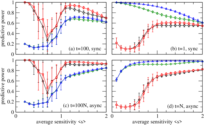
Figure 2: Quality of prediction of dynamical impact in random Boolean networks at varying average sensitivity $\langle s\rangle$. Symbols distinguish the centrality measures out-degree $d$ (green $\diamond$), strength $\sigma$ (blue $\triangle$), and the principal eigenvectors $\epsilon$ and $e$ of the activity matrix (red $\Box$) and the adjacency matrix (black $\circ$). The four panels represent combinations of long- or short-term prediction with deterministic synchronous or stochastic asynchronous update. Each data point gives the rank order correlation (cf. Methods) with dynamical impact $h(t)$, averaged over 100 independent realizations of random Boolean network with given sensitivity $\langle s\rangle$, $K=2$, and $N=500$ nodes. The error bars indicate the standard deviation over realizations.

Let us investigate the dynamical impact of nodes and its prediction by centrality measures (cf. Table 1) on random Boolean networks with $N=500$ nodes and connectivity parameter $K=2$. See Methods for details. As shown in Figure 2(a), the long-term impact of perturbations is best predicted by the leading eigenvector $\epsilon$ of the activity matrix in the whole range of sensitivity. Prediction by the leading eigenvector $e$ of the adjacency matrix is inferior to that by $\epsilon$ in the supercritical regime $\langle s\rangle>1$. When reaching $\langle s\rangle=K=2$, predictive powers become equal again, because all Boolean functions are exclusive-Or or its negation. Then all network connections have activity value 1 and adjacency and activity matrices are the same. The superiority of the eigenvector $\epsilon$ as a predictor is in agreement with the analytic arguments given in the previous section. Slightly above the critical sensitivity value 1, predictive power shows a peak for all centrality measures considered. Further analyses of the dynamics are necessary to understand the variation of the predictive power with average sensitivity, especially the minimum of $\mathcal{P}_{\epsilon}$ at $\langle s\rangle\approx 0.7$.

Figure 2(b) displays predictive power at short times, here $t=1$. As expected, strength $\sigma$ is the best predictor in this case. Predictions by the out-degree vector $d$ perform second best but significantly worse than those by strength $\sigma$.

The results in the upper panels of Fig. 2 are obtained under synchronous update of the whole system, as defined by Eq. (1). In order to check the robustness of the results, we repeat the simulations under stochastic asynchronous update according to Equation (12). The results, shown in panels (c) and (d) of Fig. 2, are qualitatively similar to those obtained under synchronous update. In the supercritical regime, however, the predictive power of all four centrality measures is increased when the updating is asynchronous instead of synchronous. Thus damage spreading is easier to predict under asynchronous update, at least with the four centrality measures studied here. This effect must be rooted in the interplay between the update order and the network structure. For instance, the damage definitely heals when the perturbed node receives the first update before all its predecessors. The frequency of this happening decreases with the out-degree $d_{i}$ and incurs an additional dependence of dynamical impact on the centrality measure $d$.

Simulations at different network sizes ($N=50$, $N=100$, not displayed) yield similar results for all four combinations of long- or short-term spreading and synchronous or asynchronous updates. The predictive power of all four centrality measures remains constant or increases with system size. Furthermore, we investigate networks with positive feedback only, i.e. without negation of signals (see Methods). For $N=500$, long-term prediction ($t=N$) and synchronous update, the predictive power $\mathcal{P}_{\epsilon}$ of the eigenvector is on average $0.80\pm 0.18$; that of strength ($\mathcal{P}_{\sigma}$) is on average $0.63\pm 0.14$.

5 Switching between attractors

Figure 3: Power of centrality measures for predicting if a perturbation changes the attractor reached. Symbols for the centrality measures are the same as in Fig. 2. Each data point is an average over 100 random Boolean networks with $N=50$ nodes and connectivity parameter $K=2$. Error bars indicate the standard deviation over the random network ensemble. Error bars are scaled down by the factor 0.2 to avoid overlapping. Additional points ($+$-symbols with dashed lines) are the fraction of realizations for which the principal eigenvector $\epsilon$ gives the best prediction of all four measures.

The long-term behaviour of Boolean dynamics is determined by attractors. These are minimal ergodic sets in state space. Under synchronous update, an attractor of length $l$ is a sequence of states $x(0),x(1),\dots,x(l-1)$ such that $f(x(t))=x([t+1]\bmod l)$ for all $t\in\{0,\dots,l-1\}$.

It is natural to ask if a perturbation in the initial condition will cause the system to arrive at a different attractor. For this investigation, we define the attractor impact $h_{i}^{\prime}$ of node $i$ as the fraction of initial conditions where a perturbation at node $i$ changes the attractor eventually reached. At difference with dynamical impact $h_{i}(t)$, attractor impact $h_{i}^{\prime}$ does not set an explicit time $t$ after which to determine the spreading or healing of the perturbation. On the other hand, $h_{i}^{\prime}$ does count the perturbation as healed whenever the perturbed and unperturbed dynamics eventually become equal up to a time lag.

Figure 3 shows the predictive power of the centrality measures for attractor impact of nodes. For averaged values, the performance comparison yields $\mathcal{P}_{\epsilon}>\mathcal{P}_{e}>\mathcal{P}_{\sigma}>\mathcal{P}_{d}$, being the same ordering as for predicting long-term dynamical impact. Due to fluctuations around the averages, this ordering does not hold for each single realization. At each considered value of the average sensitivity, a fraction at least $3/4$ of the realizations has $\epsilon$ as the best predictor. Subcritical networks, $\langle s\rangle<1$, are disregarded because here most realizations do not have more than one attractor. For $\langle s\rangle>1.7$, attractor search exceeds available computer time.

6 Dynamical impact in a real network

Table 2: Predictive power of centrality measures for the fibroblast signal transduction dynamics. The upper part of the table considers the original system. The lower part is for the system after removal of the nine nodes providing constant input. Each line of the table is a scenario defined by the update mode and the choice of long- or short-term dynamics. The bold number indicates the maximum in each line.

		all nodes
		$\mathcal{P}_{\epsilon}$	$\mathcal{P}_{e}$	$\mathcal{P}_{\sigma}$	$\mathcal{P}_{d}$
sync	$t=1$	0.671	0.454	0.930	0.455
	$t=100$	0.920	0.734	0.746	0.523
async	$t=N$	0.706	0.528	0.904	0.564
	$t=100N$	0.854	0.694	0.748	0.542

		only core nodes
		$\mathcal{P}_{\epsilon}$	$\mathcal{P}_{e}$	$\mathcal{P}_{\sigma}$	$\mathcal{P}_{d}$
sync	$t=1$	0.633	0.467	0.946	0.528
	$t=100$	0.911	0.777	0.738	0.611
async	$t=N$	0.658	0.543	0.919	0.656
	$t=100N$	0.834	0.731	0.741	0.631

Table 3: The five core nodes of the fibroblast network with the largest dynamical impact and their ranks with respect to the four centrality measures. Synchronous update is performed on the core of the network, after removal of the nine input nodes. Dynamical impact $h_{i}(t)$ measures spreading over $t=100$ time steps.

node $i$	$h_{i}(100)$	$r_{i}(\epsilon)$	$r_{i}(e)$	$r_{i}(\sigma)$	$r_{i}(d)$
Src	0.7707	1	1	1	1
B-Arrestin	0.7061	4	4	9	14
GRK	0.6458	16	27	17	43
PIP2-45	0.5961	2	12	4	4
PKC	0.5910	3	13	3	5

Let us test the performance of predictors on a non-random network now. Helikar et al. describe signal transduction in fibroblasts with a detailed Boolean network [25, 30]. The network has $N=139$ nodes and $548$ connections, including $59$ self-couplings. We choose this network because of its size and because of its large number of intertwined feedback loops of various lengths $l$, see also Figure 1 in [30]. We quantify the abundance of feedback by the trace of the $l$-th power of the adjacency matrix $A$, finding $\mathop{\rm tr}(A)=59$, $\mathop{\rm tr}(A^{2})/2=568$, $\mathop{\rm tr}(A^{3})/3=82455$ and $\mathop{\rm tr}(A^{4})/4=13921796$. The nodes fall into two classes. There are 9 input nodes with a self-coupling. Each of these applies the identity function to its own state, not receiving signals from any other node. These nodes provide constant but choosable input to the rest of the network. Each of the remaining 130 nodes receives an input from at least one other node in this set. We call these the core nodes. The in-degree of nodes varies from 1 to 14, the out-degree varies from 1 to 28.

In table 2, we summarize the predictive power of centrality measures for dynamical impact of nodes in the fibroblast network. Also for this network, the leading eigenvector $\epsilon$ of the activity matrix is the best predictor of a node’s ability to cause long-term spreading of a perturbation. Short-term spreading is best predicted by a node’s strength $\sigma_{i}$. Table 3 shows the five nodes with the largest dynamical impact and their ranks with respect to the centrality measures. Prediction of these ranks by the centrality measures is not perfect. However, the leading eigenvector $\epsilon$ of the activity matrix correctly identifies four out of the five nodes with the largest impact.

Table 3 and the lower part of Table 2 are obtained for the fibroblast network after removal of the nine input nodes. These nodes indefinitely sustain their state. Therefore a perturbation at an input node $i$ never heals, yielding maximal dynamical impact $h_{i}(t)=1$ for all times $t$. Reduction to the dynamical core by the removal of the input nodes allows for a less biased assessment of predictive power.

7 Discussion

Even in random Boolean networks, nodes exhibit significant differences in dynamical impact. These differences are captured well by local and global centrality measures. From a linearization of the dynamics, these centralities arise as column sums and eigenvectors of a network matrix. Practical applications therefore benefit from efficient computation as compared to costly direct simulation of damage spreading. For the fibroblast network, a modern workstation calculates the principal eigenvectors $\epsilon$ and $e$ in $<10^{-2}$ s, to be compared to several minutes for sampling over perturbations. Detection of attractor switching with $N=500$ nodes takes time on the order of hours, even days for some of the instances.

An important implication for networked systems is the possibility of capturing response to perturbations based on incomplete information about the system’s structure. Here, prediction of dynamical impact only uses the activity matrix while being ignorant of the actual rule tables. No distinction between positive and negative feedback enters the calculation. Comparing the case of randomly mixed feedback types to that of only one type, we find that a combination of feedback types is neither necessary nor detrimental for prediction of dynamical impact.

The scenario of predicting node impact based on partial knowledge is particularly relevant for biological systems where not all interactions are known in full detail. A large number of measures has been suggested for identifying the dynamical centers of biological systems based on the underlying network structure alone [31, 32, 33]. Most of these approaches provide only an intuitive understanding of the assumed correlation between the centrality in the network and impact on the dynamics. The present framework, beside its accuracy and computational efficiency, is based on a verifiable description of the system’s response to perturbations. In particular, it allows to distinguish between short- and long-term effects. The result is a detailed set of predictions testable in experiments. In how far the predictions meet experimental outcomes depends on the validity of idealizations at two levels: (i) the approximate analysis of dynamical impact in this letter; (ii) the Boolean idealization to capture the real system’s dynamics.

8 Methods

A random instance of a Boolean network with $N$ nodes, connectivity parameter $K$ and expected average sensitivity $\langle s\rangle$ is generated as follows. Each node $i$ is assigned a Boolean function $f_{i}$, drawn from the distribution $\pi(f)\propto\exp[\lambda s(f)]$. This distribution is normalized and supported by the set of $2^{K}$ Boolean functions with at most $K$ inputs. Here $\lambda$ is chosen such that the expectation value of $s(f)$ under the distribution $\pi$ is equal to the average sensitivity $\langle s\rangle$ [20]. Then $\pi$ is the unique distribution maximizing entropy with the given $\langle s\rangle$. For each input, on which $f_{i}$ actually depends, a link $(j,i)$ is established with the source node $j$ drawn uniformly at random. When this would lead to a duplicate or self-coupling, $j$ is discarded and redrawn. For the random networks with positive feedback only, we use $\pi(f)=0.5$ if $f$ is the AND or the OR function, $\pi(f)=0$ otherwise.

Both for the random and the empirical Boolean networks, we estimate dynamical impact of a node $i$ by $10^{4}$ runs of the dynamics. For each of these, a state $x(0)\in\{0,1\}^{N}$ is drawn uniformly. Then two replica of the system are initialized with $x(0)$ and at $(x(0))^{\updownarrow i}$. The fraction of runs where the replica are in different states at time $t$ is taken as approximation of $h_{i}(t)$. When $h_{i}(t)$ is the same for all nodes $i$ or the largest eigenvalue of the network’s activity matrix is degenerate, the network is discarded and a new independent realization is drawn. Discarding of network happens mostly at small $\langle s\rangle$. It does not occur in any of the trials with $\langle s\rangle\geq 1.2$ .

The dynamics of Equation (1) is deterministic with synchronous update. Alternatively, we consider stochastic asynchronous update as follows. At each time step $t$, a node $u(t)$ is drawn uniformly at random and the nodes take states

$$x_{i}(t+1)=\left\{\begin{array}[]{rl}f_{i}(x(t))&\textrm{if }i=u\\ x_{i}(t)&\textrm{otherwise}\end{array}\right.$$ (12)

in the subsequent time step. The same random sequence $u(t)$ of updated nodes is used for the perturbed and the unperturbed replica of the system.

We quantify the predictive power $\mathcal{P}_{y}$ of a centrality measure $y\in\{d,e,\sigma,\epsilon\}$ as the rank order correlation with dynamical impact $\mathcal{P}_{y}=\mathop{\textrm{corr}}(r(h),r(y))$ using the usual Pearson correlation coefficient $\mathop{\textrm{corr}}$. For a general vector $v=(v_{1},v_{2},\dots,v_{n})$, the rank vector $r(v)$ has entries

$$r_{i}(v)=1+|\{j\neq i|v_{j}>v_{i}\}|+\frac{1}{2}|\{j\neq i|v_{j}=v_{i}\}|~{}.$$ (13)

9 Acknowledgements

The authors thank Thomas Skodawessely for a critical reading of the draft. This work was supported financially by VolkswagenStiftung.

References

- [1] \NameKauffman S. A. \REVIEWJ Theor Biol221969437.
- [2] \NameKauffman S. A. \BookThe Origins of Order (Oxford University Press, New York) 1993.
- [3] \Namede Jeong H. \REVIEWJ Comput Biol9200267.
- [4] \NameBornholdt S. \REVIEWScience3102005449.
- [5] \NameAldana M., Coppersmith S. Kadanoff L. \REVIEWPerspectives and Problems in Nonlinear Science200323.
- [6] \NameDrossel B. \REVIEWReviews of Nonlinear Dynamics and Complexity1200769.
- [7] \NameMihaljev T. Drossel B. \REVIEWPhys. Rev. E742006046101.
- [8] \NameSzejka A., Mihaljev T. Drossel B. \REVIEWNew J. Phys.102008063009.
- [9] \NameAldana M. Cluzel P. \REVIEWProc. Natl. Acad. Sci. U.S.A.10020038710.
- [10] \NameDrossel B. Greil F. \REVIEWPhys. Rev. E802009026102.
- [11] \NameSocolar J. E. S. Kauffman S. A. \REVIEWPhys. Rev. Lett.902003068702.
- [12] \NameSamuelsson B. Troein C. \REVIEWPhys. Rev. Lett.902003098701.
- [13] \NameKlemm K. Bornholdt S. \REVIEWPhys. Rev. E722005055101.
- [14] \NameDerrida B. Pomeau Y. \REVIEWEurophys Lett1198645.
- [15] \NameShmulevich I., Lähdesmäki H., Dougherty E. R., Astola J. Zhang W. \REVIEWProc. Natl. Acad. Sci. U.S.A.100200310734.
- [16] \NameFretter C., Szejka A. Drossel B. \REVIEWNew J. Phys.112009033005.
- [17] \NamePeixoto T. P. \REVIEWPhys. Rev. Lett.1042010048701.
- [18] \NameSchmal C., Peixoto T. P. Drossel B. \REVIEWNew J. Phys.122010113054.
- [19] \NameMozeika A. Saad D. \REVIEWPhys. Rev. Lett.1062011214101.
- [20] \NameGhanbarnejad F. Klemm K. \REVIEWPhys. Rev. Lett.1072011188701.
- [21] \NameSeshadhri C., Vorobeychik Y., Mayo J. R., Armstrong R. C. Ruthruff J. R. \REVIEWPhys. Rev. Lett.1072011108701.
- [22] \NameKauffman S., Peterson C., Samuelsson B. Troein C. \REVIEWProc. Natl. Acad. Sci. U.S.A.100200314796.
- [23] \NameAlbert R. Othmer H. \REVIEWJ Theor Biol22320031.
- [24] \NameLi F., Long T., Lu Y., Ouyang Q. Tang C. \REVIEWProc Natl Acad Sci USA10120044781.
- [25] \NameHelikar T., Konvalina J., Heidel J. Rogers J. A. \REVIEWProc Natl Acad Sci USA10520081913.
- [26] \NameAlbert I., Thakar J., Li S., Zhang R. Albert R. \REVIEWSource Code Biol Med3200816.
- [27] \NameDavidich M. I. Bornholdt S. \REVIEWPLoS One32008e1672.
- [28] \NameDavidich M. Bornholdt S. \REVIEWJ. Theor. Biol.2552008269 .
- [29] \NameXia Q., Liu L., Ye W. Hu G. \REVIEWNew J. Phys.132011083002.
- [30] \NameRue P., Pons A. J., Domedel-Puig N. Garcia-Ojalvo J. \REVIEWChaos202010045110.
- [31] \NameWuchty S. Stadler P. F. \REVIEWJ. Theor. Biol.223200345.
- [32] \NameKitsak M., Gallos L., Havlin S., Liljeros F., Muchnik L., Stanley H. Makse H. \REVIEWNature Physics62010888.
- [33] \NameKlemm K., Serrano M. A., Eguiluz V. M. San Miguel M. \REVIEWSci. Rep.22012292.