Incorporating biological information into linear models: A Bayesian approach to the selection of pathways and genes

Abstract

The vast amount of biological knowledge accumulated over the years has allowed researchers to identify various biochemical interactions and define different families of pathways. There is an increased interest in identifying pathways and pathway elements involved in particular biological processes. Drug discovery efforts, for example, are focused on identifying biomarkers as well as pathways related to a disease. We propose a Bayesian model that addresses this question by incorporating information on pathways and gene networks in the analysis of DNA microarray data. Such information is used to define pathway summaries, specify prior distributions, and structure the MCMC moves to fit the model. We illustrate the method with an application to gene expression data with censored survival outcomes. In addition to identifying markers that would have been missed otherwise and improving prediction accuracy, the integration of existing biological knowledge into the analysis provides a better understanding of underlying molecular processes.

, ,
and m5Supported in part by NIH Grant R01-HG0033190-05 and NSF Grant DMS-10-07871.

1 Introduction

DNA microarrays have been used successfully to identify gene expression signatures characteristic of disease subtypes [Golub et al. (1999)] or distinct outcomes to therapy [Shipp et al. (2002)]. Many statistical methods have been developed to select genes for disease diagnosis, prognosis and therapeutic targets. However, gene selection alone may not be sufficient. In cancer pharmacogenomics, for instance, cancer drugs are increasingly designed to target specific pathways to account for the complexity of the oncogenic process and the complex relationships between genes [Downward (2006)]. Metabolic pathways, for example, are defined as a series of chemical reactions in a living cell that can be activated or inhibited at multiple points. If a gene at the top of a signaling cascade is selected as a target, it is not guaranteed that the reaction will be successfully inactivated, because multiple genes downstream can still be activated or inhibited. Signals are generally relayed via multiple signaling routes or networks. Even if a branch of the pathway is completely blocked by inhibition or activation of multiple genes, the signal may still be relayed through an alternative branch or even through a different pathway [Bild et al. (2006)]. Downward (2006) pointed out that targeting a single pathway or a few signaling pathways might not be sufficient. Thus, the focus is increasingly on identifying both relevant genes and pathways. Genes and/or gene products generally interact with one another and they often function together concertedly. Here we propose a Bayesian model that addresses this question by incorporating information of pathway memberships and gene networks in the analysis of DNA microarray data. Such information is used to define pathway summaries, specify prior distributions, and structure the MCMC moves.

Several public and commercial databases have been developed to structure and store the vast amount of biological knowledge accumulated over the years into functionally or biochemically related groups. These databases focus on describing signaling, metabolic or regulatory pathways. Some examples include Gene Ontology (GO) [Ashburner et al. (2000)], Kyoto Encyclopedia of Genes and Genomes (KEGG) [Kanehisa and Goto (2000)], MetaCyc [Krieger et al. (2004)], PathDB, Reactome KnowledgeBase [Joshi-Tope et al. (2005)], Invitrogen iPath (www.invitrogen.com) and Cell Signaling Technology (CST) Pathway (www.cellsignal.com). The need to integrate gene expression data with the biological knowledge accumulated in these databases is well recognized. Several software packages that query pathway information and overlay DNA microarray data on pathways have been developed. Nakao et al. (1999) implemented a visualization tool that color-codes KEGG pathway diagrams to reflect changes in their gene expression levels. GenMAPP [Dahlquist et al. (2002)] is another graphical tool that allows visualization of microarray data in the context of biological pathways or any other functional grouping of genes. Doniger et al. (2003) use GenMAPP to view genes involved in specific GO terms. Another widely used method that relates pathways to a set of differentially expressed genes is the gene set enrichment analysis (GSEA) [Subramanian et al. (2005)]. Given a list of genes, GSEA computes an enrichment score to reflect the degree to which a predefined pathway is over-represented at the top or bottom of the ranked list. These procedures are useful starting points to observe gene expression changes for known biological processes.

Recent studies have gone a step further and focused on incorporating pathway information or gene–gene network information into the analysis of gene expression data. For example, Park, Hastie and Tibshirani (2007) have attempted to incorporate GO annotation to predict survival time, first grouping genes based on their GO membership, calculating the first principal component to form a super-gene within each cluster and then applying a Cox model with $L_{1}$ penalty to identify super-genes, that is, GO terms related to the outcome. Wei and Li (2007) have considered a small set of 33 preselected signaling pathways and used the implied relationships among genes to infer differentially expressed genes, and Wei and Li (2008) have extended this work by including a temporal dimension. Li and Li (2008) and Pan, Xie and Shen (2010) have proposed different procedures that use the gene–gene network to build penalties in a regression model for gene selection. Bayesian approaches have also been developed. Li and Zhang (2010) have incorporated the dependence structure of transcription factors in a regression model with gene expression outcomes. There, a network is defined based on the Hamming distance between candidate motifs and used to specify a Markov random field prior for the motif selection indicator. Telesca et al. (2008) have proposed a model for the identification of differentially expressed genes that takes into account the dependence structure among genes from available pathways while allowing for correction in the gene network topology. Stingo and Vannucci (2011) use a Markov random field prior that captures the gene–gene interaction network in a discriminant analysis setting.

These methods use the gene-pathway relationships or gene network information to identify either the important pathways or the genes. Our goal is to develop a more comprehensive method that selects both pathways and genes using a model that incorporates pathway-gene relationships and gene dependence structures. In order to identify relevant genes and pathways, latent binary vectors are introduced and updated using a two-stage Metropolis–Hastings sampling scheme. The gene networks are used to define a Markov random field prior on the gene selection indicators and to structure the Markov chain Monte Carlo (MCMC) moves. In addition, the pathway information is used to derive pathway expression measures that summarize the group behavior of genes within pathways. In this paper we make use of the first latent components obtained by applying partial least squares (PLS) regressions on the selected genes from each pathway. PLS is an efficient statistical regression technique that was initially proposed in the chemometrics literature [Wold (1966)] and more recently used for the analysis of genomic and proteomic data; see Boulesteix and Strimmer (2007). We apply the model to simulated and real data using the pathway structure from the KEGG database.

Our simulation studies show that the MRF prior leads to a better separation between relevant and nonrelevant pathways, and to less false positives in a model with fairly small regression coefficients. Other authors have reported similar results. Li and Zhang (2010), in particular, comment on the effect of the MRF prior on the selection power in their linear regression setting. They also notice that adding the MRF prior implies a relatively small increase in computational cost. Wei and Li (2007, 2008) report that their method is quite effective in identifying genes and modified subnetworks and that it has higher sensitivity than commonly used procedures that do not use the pathway structure, with similar and, in some cases, lower false discovery rates. Furthermore, in our model formulation we use the network information not only for prior specification but also to structure the MCMC moves. This is helpful for arriving at promising models faster by proposing relevant configurations. In real data applications the integration of pathway information may allow the identification of relevant predictors that could be missed otherwise, aiding the interpretation of the results, in particular, for the selected genes that are connected in the MRF, and also improving the prediction accuracy of selected models.

The paper is organized as follows. Section 2 contains the model formulation and prior specification. Section 3 describes the MCMC procedure and strategies for posterior inference. In Section 4 performances are evaluated on simulated data and an application of the method to gene expression data with survival outcomes is presented. Section 5 concludes the paper with a brief discussion.

2 Model specification

We describe how we incorporate pathway and gene network information into a Bayesian modeling framework for gene and pathway selection. Figure 1 represents a schematic representation of our approach and model.

2.1 Regression on latent measures of pathway activity

Our goal is to build a model for identifying pathways related to a particular phenotype while simultaneously locating genes from these selected pathways that are involved in the biological process of interest. The data we have available for analysis consist of the following: [(4)]

$Y$, an $n\times 1$ vector of outcomes.

$\mathbf{X}$, an $n\times p$ matrix of gene expression levels. Without loss of generality, $\mathbf{X}$ is centered so that its columns sum to 0.

$\mathbf{S}$, a $K\times p$ matrix indicating membership of genes in pathways, with elements $s_{kj}=1$ if gene $j$ belongs to pathway $k$, and $s_{kj}=0$ otherwise.

$\mathbf{R}$, a $p\times p$ matrix describing relationships between genes, with $r_{ij}=1$ if genes $i$ and $j$ have a direct link in the gene network, and $r_{ij}=0$ otherwise. The matrices $\mathbf{S}$ and $\mathbf{R}$ are constructed using information retrieved from pathway databases; see the application in Section 4.2 for details.

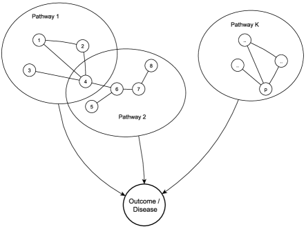
Figure 1: Schematic representation of our proposed approach. Information on known pathways and gene–gene networks is obtained from available databases. PLS components restricted to known pathways serve as possible regressors to predict a disease outcome, according to model (1). The goal of the inference is to identify the pathways to be included in the model and the genes to be included within those pathways.

Since the goal of the analysis is to study the association between the response variable and the pathways, we need to derive a score as a measure of “pathway expression” that summarizes the group behavior of included genes within pathways. We do this by using the latent components from a PLS regression of $Y$ on selected subsets of genes from each pathway. A number of recent studies have, in fact, applied dimension reduction techniques to capture the group behavior of multiple genes. Pittman et al. (2004), for instance, first apply $k$-means clustering to identify subsets of potentially related genes, then use as regressors the first principal components obtained from applying principal component analysis (PCA) to each cluster. Bair et al. (2006) start by removing genes that have low univariate correlation with the outcome variable, then apply PCA on the remaining genes to form clusters or conceptual pathways, which are used as regressors. In our method, instead of attempting to infer conceptual pathways, we use the existing pathway information. We compute a pathway activity measure by applying PLS regression of $Y$ on a subset of selected genes from the pathway. PLS has the advantage of taking into account the covariance between regressors and the response variable $Y$, whereas PCA focuses solely on the variability in the covariate data. The selection of a subset of gene expressions to form the PLS components is similar in spirit to the sparse PCA method proposed by Zou, Hastie and Tibshirani (2006), which selects variables to form the principal components.

To identify both relevant groups and important genes, we introduce two binary vector indicators, a $K\times 1$ vector $\bolds\theta$ for the inclusion of the groups and a $p\times 1$ vector $\bolds\gamma$ for the inclusion of genes, that is, $\gamma_{j}=1$ if gene $j$ is selected for at least one pathway score, and $\gamma_{j}=0$ otherwise. Assuming that the response $Y$ is continuous, the linear regression model that relates $Y$ to the selected pathways and genes is

$$Y={\mathbf{1}}\alpha+\sum_{k=1}^{K_{\theta}}T_{k(\gamma)}\beta_{k(\gamma)}+\bolds\varepsilon,\qquad\bolds\varepsilon\sim\mathcal{N}({\mathbf{0}},\sigma^{2}\mathbf{I}),$$ (1)

where $K_{\theta}=\sum_{k=1}^{K}\theta_{k}$ is the number of selected pathways and where $T_{k(\gamma)}$ corresponds to the first latent PLS component generated based on the expression levels of selected genes belonging to pathway $k$, that is, using the $X_{j}$’s corresponding to $s_{kj}=1$ and $\gamma_{j}=1$. To be more precise, let pathway $k$ contain $p_{k}=\sum_{j=1}^{p}s_{kj}$ genes and let $p_{k\gamma}=\sum_{j=1}^{p}s_{kj}\gamma_{j}$ denote the number of selected genes (i.e., genes included in the model) that belong to pathway $k$. Then $T_{k(\gamma)}$ corresponds to the first latent PLS component generated by applying PLS to the expression data of the $p_{k\gamma}$ genes, denoted as $\mathbf{X}_{k(\gamma)}$,

$$T_{k(\gamma)}=\mathbf{X}_{k(\gamma)}U_{1},$$

where $U_{1}$ is the $p_{k\gamma}\times 1$ eigenvector corresponding to the largest eigenvalue of $C_{xy}C_{xy}^{T}$, with $C_{xy}=\operatorname{cov}(\mathbf{X}_{k(\gamma)},Y)$ [see, e.g., Lindgren, Geladi and Wold (1993)]. Thus, $T_{k}(\gamma)$ is an $n\times 1$ vector and $\beta_{k}(\gamma)$ is a scalar. Model (1) can therefore be seen as a PLS regression model with PLS components restricted to available pathways, and where the goal of the inference is to identify the pathways to be included in the model, and the genes to be included within those pathways.

2.2 Models for categorical or censored outcomes

In the construction above, we have assumed a continuous response. However, our model formulation can easily be extended to handle categorical or censored outcome variables.

When $Y$ is a categorical variable taking one of $G$ possible values, $0,\ldots,\allowbreak G-1$, a probit model can be used, as done by Albert and Chib (1993), Sha et al. (2004) and Kwon et al. (2007). Briefly, each outcome $Y_{i}$ is associated with a vector $(p_{i,0},\ldots,p_{i,G-1})$, where $p_{ig}=P(Y_{i}=g)$ is the probability that subject $i$ falls in the $g$th category. The probabilities $p_{ig}$ can be related to the linear predictors using a data augmentation approach. Let $\mathbf{Z}_{i}$ be latent data corresponding to the unobserved propensities of subject $i$ to belong to one of the classes. When the observed outcomes $Y_{i}$ correspond to nominal values, the relationship between $Y_{i}$ and $\mathbf{Z}_{i}=(z_{i,1},\ldots,z_{i,G-1})$ can be defined as

$$Y_{i}=\cases{\displaystyle 0,&\quad if $\displaystyle\max_{1\leq l\leq G-1}\{z_{i,l}\}\leq 0$,\vspace*{2pt}\cr\displaystyle g,&\quad if $\displaystyle\max_{1\leq l\leq G-1}\{z_{i,l}\}>0$ and $\displaystyle z_{i,g}=\max_{1\leq l\leq G-1}\{z_{i,l}\}$.}$$ (2)

A multivariate normal model can then be used to associate $\mathbf{Z}_{i}$ to the predictors

$$\mathbf{Z}_{i}={\mathbf{1}}\alpha+\sum_{k=1}^{K_{\theta}}T_{i,k(\gamma)}\bolds\beta_{k(\gamma)}+\bolds\varepsilon_{i},\qquad\bolds\varepsilon_{i}\sim\mathcal{N}(0,\bolds\Sigma),i=1,\ldots,n.$$ (3)

If the observed outcomes $Y_{i}$ correspond, instead, to ordinal categories, the latent variable $Z_{i}$ is defined such that $Y_{i}=g$ if $\delta_{g}<Z_{i}\leq\delta_{g+1}$, $g=0,\ldots,G-1$, where the boundaries $\delta_{g}$ are unknown and $-\infty=\delta_{0}<\delta_{1}<\cdots<\delta_{G-1}<\delta_{G}=\infty$. The latent variable $Z_{i}$ is associated with the predictors through the linear model

$$Z_{i}=\alpha+\sum_{k=1}^{K_{\theta}}T_{i,k(\gamma)}\beta_{k(\gamma)}+\varepsilon_{i},\qquad\varepsilon_{i}\sim\mathcal{N}(0,\sigma^{2}),i=1,\ldots,n.$$ (4)

For censored survival outcomes, an accelerated failure time (AFT) model can be used [Wei (1992); Sha, Tadesse and Vannucci (2006)]. In this case, the observed data are $Y_{i}=\min(T_{i},C_{i})$ and $\delta_{i}=I\{Y_{i}\leq C_{i}\}$, where $T_{i}$ is the survival time for subject $i$, $C_{i}$ is the censoring time, and $\delta_{i}$ is a censoring indicator. A data augmentation approach can be used and latent variables $Z_{i}$ can be introduced such that

$$\cases{\displaystyle Z_{i}=\log(Y_{i}),&\quad if $\delta_{i}=1$,\cr\displaystyle Z_{i}>\log(Y_{i}),&\quad if $\delta_{i}=0$.}$$ (5)

The AFT model can then be written in terms of the latent $Z_{i}$ similarly to (4) where the $\varepsilon_{i}$’s are independent and identically distributed random variables that may take one of several parametric forms. Sha, Tadesse and Vannucci (2006) consider cases where $\varepsilon_{i}$ follows a normal or a $t$-distribution.

2.3 Prior for regression parameters

The regression coefficient $\beta_{k}$ in (1) measures the effect of the PLS latent component summarizing the effect of pathway $k$ on the response variable. However, not all pathways are related to the phenotype and the goal is to identify the predictive ones. Bayesian methods that use mixture priors for variable selection have been thoroughly investigated in the literature, in particular, for linear models; see George and McCulloch (1997) for multiple regression, Brown, Vannucci and Fearn (1998) for extensions to multivariate responses and Sha et al. (2004) for probit models. A comprehensive review on features of the selection priors and on computational aspects of the method can be found in Chipman, George and McCulloch (2001). Similarly, we use the latent vector $\bolds\theta$ to specify a scale mixture of a normal density and a point mass at zero for the prior on each $\beta_{k}$ in (1):

$$\beta_{k}|\theta_{k},\sigma^{2}\sim\theta_{k}\cdot\mathcal{N}(\beta_{0},h\sigma^{2})+(1-\theta_{k})\cdot\delta_{0}(\beta_{k}),\qquad k=1,\ldots,K,$$ (6)

where $\delta_{0}(\beta_{k})$ is a Dirac delta function. The hyperparameter $h$ in (6) regulates, together with the hyperparameters of $p(\bolds\theta,\bolds\gamma|\eta)$ defined in Section 2.4 below, the amount of shrinkage in the model. We follow the guidelines provided by Sha et al. (2004) and specify $h$ in the range of variability of the data so as to control the ratio of prior to posterior precision. For the intercept term, $\alpha$, and the variance, $\sigma^{2}$, we take conjugate priors $\alpha|\sigma^{2}\sim\mathcal{N}(\alpha_{0},h_{0}\sigma^{2})$ and $\sigma^{2}\sim\operatorname{Inv\mbox{-}Gamma}(\nu_{0}/2,\nu_{0}\sigma_{0}^{2}/2)$, where $\alpha_{0}$, $\beta_{0}$, $h_{0}$, $h$, $\nu_{0}$ and $\sigma^{2}_{0}$ are to be elicited.

2.4 Priors for pathway and gene selection indicators

In this section we define the prior distributions for the pathway selection indicator, $\bolds\theta$, and gene selection indicator, $\bolds\gamma$. These priors are first defined marginally then jointly, taking into account some necessary constraints.

Each element of the latent $K$-vector $\bolds\theta$ is defined as

$$\theta_{k}=\cases{\displaystyle 1,&\quad if pathway $k$ is represented in the model,\cr\displaystyle 0,&\quad otherwise}$$ (7)

for $k=1,\ldots,K$. We assume independent Bernoulli priors for the $\theta_{k}$’s,

$$p(\bolds\theta|\varphi_{k})=\prod_{k=1}^{K}\varphi_{k}^{\theta_{k}}(1-\varphi_{k})^{1-\theta_{k}},$$ (8)

where $\varphi_{k}$ determines the proportion of pathways expected a priori in the model. A mixture prior can be further specified for $\varphi_{k}$ to achieve a better discrimination in terms of posterior probabilities between significant and nonsignificant pathways by inflating $p(\theta_{k}=0)$ toward 1 for the nonrelevant pathways, as first suggested by Lucas, Carvalho, Wang, Bild, Nevins and West (2006),

$$p(\varphi_{k})=\rho\delta_{0}(\varphi_{k})+(1-\rho)\mathcal{B}(\varphi_{k}|a_{0},b_{0}),$$ (9)

where $\mathcal{B}(\varphi_{k}|a_{0},b_{0})$ is a Beta density function with parameters $a_{0}$ and $b_{0}$. Since inference on $\varphi_{k}$ is not of interest, it can be integrated out to simplify the MCMC implementation. This leads to the following marginal prior for $\bolds\theta$:

$$p(\bolds\theta)=\prod_{k}\biggl{[}\rho\cdot(1-\theta_{k})+(1-\rho)\cdot\frac{B(a_{0}+\theta_{k},b_{0}+1-\theta_{k})}{B(a_{0},b_{0})}\biggr{]},$$ (10)

where $B(\cdot,\cdot)$ is the Beta function. Prior (10) corresponds to a product of Bernoulli distributions with parameter $\varphi_{k}^{*}=\frac{a_{0}(1-\rho)}{a_{0}+b_{0}}$.

For the latent $p$-vector $\bolds\gamma$ we specify a prior distribution that is able to take into account not only the pathway membership of each gene but also the biological relationships between genes within and across pathways, which are captured by the matrix $R$. Following Li and Zhang (2010), we model these relations using a Markov random field (MRF), where genes are represented by nodes and relations between genes by edges. A MRF is a graphical model in which the distribution of a set of random variables follow Markov properties that can be described by an undirected graph. In particular, two unconnected genes are considered conditionally independent given all other genes [Besag (1974)]. Relations on the MRF are represented by the following probabilities:

$$p(\gamma_{j}|\eta,\gamma_{i},i\in N_{j})=\frac{\exp(\gamma_{j}F(\gamma_{j}))}{1+\exp(F(\gamma_{j}))},$$ (11)

where $F(\gamma_{j})=(\mu+\eta\sum_{i\in N_{j}}\gamma_{i}))$ and $N_{j}$ is the set of direct neighbors of gene $j$ in the MRF using only pathways represented in the model, that is, pathways with $\theta_{k}=1$. The corresponding global distribution on the MRF is given by

$$p(\bolds\gamma|{\bolds\theta},\mu,\eta)\propto\exp(\mu\mathbf{1}_{p}^{\prime}\bolds\gamma+\eta\bolds\gamma^{\prime}\mathbf{R}\bolds\gamma),$$ (12)

with $\mathbf{1}_{p}$ the unit vector of dimension $p$ and $\mathbf{R}$ the matrix introduced in Section 2.1. The parameter $\mu$ controls the sparsity of the model, while $\eta$ regulates the smoothness of the distribution of ${\bolds\gamma}$ over the graph by controlling the prior probability of selecting a gene based on how many of its neighbors are selected. In particular, higher values of $\eta$ encourage the selection of genes with neighbors already selected into the model. If a gene does not have any neighbor, then its prior distribution reduces to an independent Bernoulli with parameter $p=\exp(\mu)/[1+\exp(\mu)]$, which is a logistic transformation of $\mu$.

Here, unlike Li and Zhang (2010), who fix both parameters of the MRF prior, we specify a hyperprior for $\eta$. We give positive probability to values of $\eta$ bigger than $0$, which is biologically more intuitive than negative values of this parameter (which would favor neighboring genes to have different inclusion status). Such restriction on the domain of $\eta$ also minimizes the “phase transition” problem that typically occurs with MRF parameterizations of type (11), where the dimension of the selected model increases massively for small increments of $\eta$. When the phase transition occurs the number of selected genes increases substantially. Here, after having detected the phase transition value $\eta_{PT}$, by simulating from (12) over a grid of $\eta$ values, we specify a Beta distribution $\operatorname{Beta}(c_{0},d_{0})$ on $\eta/\eta_{PT}$.

Constraints need to be imposed to ensure both interpretability and identifiability of the model. We essentially want to avoid the following: [(3)]

empty pathways, that is, selecting a pathway but none of its member genes;

orphan genes, that is, selecting a gene but none of the pathways that contain it;

selection of identical subsets of genes by different pathways, a situation that generates identical values $T_{k(\gamma)}$ and $T_{k^{\prime}(\gamma)}$ to be included in the model. These constraints imply that some combinations of $\bolds\theta$ and $\bolds\gamma$ values are not allowed. The joint prior probability for $(\bolds\theta,\bolds\gamma)$ taking into account these constraints is given by

$$p(\bolds\theta,\bolds\gamma|\eta)\propto\cases{\displaystyle\prod_{k=1}^{K}\varphi_{k}^{*\theta_{k}}(1-\varphi_{k}^{*})^{1-\theta_{k}}\exp(\mu\mathbf{1}_{p}^{\prime}\bolds\gamma+\eta\bolds\gamma^{\prime}\mathbf{R}\bolds\gamma),\cr\qquad\mbox{for valid configurations,}\cr 0,\quad\mbox{for invalid configurations.}}$$

3 Model fitting

We now describe our MCMC procedure to fit the model and discuss strategies for posterior inference with huge posterior spaces, as in this model. In the Bayesian literature on variable selection for standard linear regression models stochastic search algorithms have been designed to explore the posterior space, and have been successfully employed in genomic applications with prohibitive settings, handling models with thousands of genes. A key to these applications is the assumption of sparsity of the model, that is, the belief that the response is associated with a small number of regressors. A stochastic search then allows one to explore the posterior space in an effective way, quickly finding the most probable configurations, that is, those corresponding to coefficients with high marginal probabilities, while spending less time in regions with low posterior probability.

We describe below the MCMC algorithm we have designed for our problem. In particular, borrowing from the literature on stochastic searches for variable selection, we work with a marginalized model and design a Metropolis–Hastings algorithm that updates the indicator parameters for the inclusion of pathways and genes with a set of moves that add and/or delete a single gene and a single pathway. Also, we update the parameter $\eta$ of the MRF from its posterior distribution by employing the general method proposed by Møller et al. (2006). In Stingo et al. (2011) we discuss how our Bayesian stochastic search variable selection kernel generates an ergodic Markov chain over the restricted space. In applications, we have found that a good way to asses if the stochastic exploration can be considered satisfactory is to check the concordance of the posterior probabilities obtained from different chains started from different initial points.

3.1 Marginal posterior probabilities

The model parameters consist of $(\alpha,\bolds\beta,$ $\sigma^{2},{\bolds\gamma},\bolds\theta,\eta)$. The MCMC procedure can be made more efficient by integrating out some of the parameters. Here, we integrate out the regression parameters, $\alpha$, $\bolds\beta$ and $\sigma^{2}$. This leads to a multivariate $t$-distribution

$$\hskip 24.0ptf(Y|\mathbf{T},\bolds\theta,\bolds\gamma)\!\sim\!\mathcal{T}_{\nu_{0}}\bigl{(}\alpha_{0}\mathbf{1}_{n}\!+\!\mathbf{T}_{(\theta,\gamma)}\beta_{0},\sigma_{0}^{2}\bigl{(}\mathbf{I}_{n}\!+\!h_{0}\mathbf{1}_{n}\mathbf{1}_{n}^{\prime}\!+\!\mathbf{T}_{(\theta,\gamma)}\bolds\Sigma_{0}\mathbf{T}_{(\theta,\gamma)}^{\prime}\bigr{)}\bigr{)},$$ (13)

with $\nu_{0}$ degrees of freedom and $\mathbf{1}_{n}$ an $n$-vector of ones, and where $\bolds\Sigma_{0}=h\mathbf{I}_{K_{\theta}}$, with $\mathbf{I}_{n}$ the $n\times n$ identity matrix, and ${\mathbf{T}}_{(\theta,\gamma)}$ the $n\times K_{\theta}$ matrix derived from the first PLS latent components for the selected pathways using the selected genes. In the notation (13) the two arguments of the $t$-distribution represent the mean and the scale parameter of the distribution, respectively. The posterior probability distribution of the pathway and gene selection indicators is then given by

$$f(\bolds\theta,\bolds\gamma,\eta|\mathbf{T},Y)\propto f(Y|\mathbf{T},\bolds\theta,\bolds\gamma)\cdot p(\bolds\theta,\bolds\gamma|\eta)\cdot p(\eta).$$ (14)

3.2 MCMC sampling

The MCMC steps consist of the following: (I) sampling pathway and gene selection indicators from $p(\bolds\theta,\bolds\gamma|\mbox{rest})$; (II) sampling the MRF parameter from $p(\eta|\mbox{rest})$; (III) sampling additional parameters introduced when fitting probit models for categorical outcomes or AFT models for survival data.

1. [(III)]

2. The parameters $(\bolds\theta,\bolds\gamma)$ are updated using a Metropolis–Hastings algorithm in a two-stage sampling scheme. The pathway-gene relationships are used to structure the moves and account for the constraints specified in Section 2.4. Details of the MCMC moves to update $(\bolds\theta,\bolds\gamma)$ are given in Stingo et al. (2011). They consist of randomly choosing one of the following move types:

   1. [(3)]

   2. change the inclusion status of gene and pathway by randomly choosing between adding a pathway and a gene or removing them both;

   3. change the inclusion status of gene but not pathway by randomly choosing between adding a gene or removing a gene;

   4. change the inclusion status of pathway but not gene by randomly choosing between adding a pathway or removing a pathway.

3. At this step we want to draw the MRF parameter $\eta$ from the posterior density $p(\eta|\bolds\gamma)\propto p(\eta)p(\bolds\gamma|\eta)$. The prior distribution on $\bolds\gamma$ is of the form

   $$p(\bolds\gamma|\eta)=q_{\eta}(\bolds\gamma)/Z_{\eta}$$ (15)

   with unnormalized density $q_{\eta}(\bolds\gamma)$ and a normalizing constant $Z_{\eta}$ which is not available analytically. When calculating the Metropolis–Hastings ratio to determine the acceptance probability of a new value $\eta^{p}$,

   $$H(\eta^{p}|\eta^{o})=\frac{p(\eta^{p})q_{\eta^{p}}(\bolds\gamma)q(\eta^{o}|\eta^{p})}{p(\eta^{o})q_{\eta^{o}}(\bolds\gamma)q(\eta^{p}|\eta^{o})}\bigg{/}\frac{Z_{\eta^{p}}}{Z_{\eta^{o}}},$$ (16)

   with $\eta^{o}$ the current value for $\eta$, one needs to take into account that $Z_{\eta^{p}}/Z_{\eta^{o}}\neq 1$. Following Møller et al. (2006), we introduce an auxiliary variable $w$, defined on the same state space as that of $\bolds\gamma$, which has conditional density $f(w|\eta,\bolds\gamma)$, and consider the posterior $p(\eta,w|\bolds\gamma)\propto f(w|\eta,\bolds\gamma)p(\eta)q_{\eta}(\bolds\gamma)/Z_{\eta}$, which of course still involves the unknown $Z_{\eta}$. Obviously, marginalization over $w$ of $p(\eta,w|\bolds\gamma)$ gives the desired distribution $p(\eta|\bolds\gamma)$. Now, if $(\eta^{o},w^{o})$ is the current state of the algorithm, we first propose $\eta^{p}$ with density $q(\eta^{p}|\eta^{o})$, then $w^{p}$ with density $q(w^{p}|w^{o},\eta^{p},\eta^{o})$. As usual, the choice of these proposal densities is arbitrary from the point of view of the equilibrium distribution of the chain of $\eta$ values. The choice of $f(w|\eta,\bolds\gamma)$ is also arbitrary. The key idea of the method proposed by Møller et al. (2006) is to take the proposal density for the auxiliary variable $w$ to be of the same form as (15), but dependent on $\eta^{p}$ rather than $\eta^{o}$, that is,

   $$q(w^{p}|w^{o},\eta^{p},\eta^{o})=p(w^{p}|\eta^{p})=q_{\eta^{p}}(w^{p})/Z_{\eta^{p}}.$$ (17)

   Then the Metropolis–Hastings ratio becomes

   $$H(\eta^{p},w^{p}|\eta^{o},w^{o})=\frac{f(w^{p}|\eta^{p},\bolds\gamma)p(\eta^{p})q_{\eta^{p}}(\bolds\gamma)q_{\eta^{o}}(w^{o})q(\eta^{o}|\eta^{p})}{f(w^{o}|\eta^{o},\bolds\gamma)p(\eta^{o})q_{\eta^{o}}(\bolds\gamma)q_{\eta^{p}}(w^{p})q(\eta^{p}|\eta^{o})},$$ (18)

   and no longer depends on $Z_{\eta^{p}}/Z_{\eta^{o}}$. The new value $w^{p}$ for the auxiliary variable $w$ is drawn from (17) by perfect simulation using the algorithm proposed by Propp and Wilson (1996).

4. In the case of classification or survival outcomes, the augmented data $Z$ need to be updated from their full conditionals using Gibbs sampling; see Sha et al. (2004), Sha, Tadesse and Vannucci (2006) and Kwon et al. (2007) for details.

3.3 Posterior inference

The MCMC procedure results in a list of visited models with included pathways indexed by $\bolds\theta$ and selected genes indexed by $\bolds\gamma$, and their corresponding relative posterior probabilities. Pathway selection can be based on the marginal posterior probabilities $p(\theta_{k}|\mathbf{T},Y)$. A simple strategy is to compute Monte-Carlo estimates by counting the number of appearances of each pathway across the visited models. Relevant pathways are identified as those with largest marginal posterior probabilities. Then relevant genes from these pathways are identified based on their marginal posterior probabilities conditional on the inclusion of a pathway of interest, $p(\gamma_{j}|\mathbf{T},Y,I{\{\theta_{k}s_{kj}=1\}})$. An alternative inference for gene selection is to focus on a subset of pathways, $\mathcal{P}$, and consider the marginal posterior probability conditional on at least one pathway the gene belongs to being represented in the model, $p(\gamma_{j}|\mathbf{T},Y,I{\{\sum_{k\in\mathcal{P}}\theta_{k}s_{kj}>0\}})$. We note that Rao–Blackwellized estimates have been employed in standard linear regression models, in place of frequency estimates, by averaging the full conditional posterior probabilities of the inclusion indicators. These estimates are computationally quite expensive, though they may have better precision, as noted by Guan and Stephens (2011). Because of our strategy for inference, that selects first pathways and then genes conditional on selected pathways, Rao–Blackwellized estimates of marginal probabilities may not be straightforward to derive. In all simulations and examples reported in this paper we have obtained satisfactory results by simply estimating the marginal posterior probabilities with the corresponding relative frequencies of inclusion in the visited models.

Inference for a new set of observations, $(\mathbf{X}_{f},Y_{f})$, can be done via least squares prediction, $\widehat{Y}_{f}=\mathbf{1}_{n}\tilde{\alpha}+\mathbf{T}_{f(\theta,\gamma)}\tilde{\bolds\beta}_{(\theta,\gamma)}$, where $\mathbf{T}_{f(\theta,\gamma)}$ is the first principal component based on selected genes from relevant pathways and where $\tilde{\alpha}=\bar{Y}$ and $\tilde{\bolds\beta}_{(\theta,\gamma)}=(\mathbf{T}_{(\theta,\gamma)}^{\prime}{\mathbf{T}}_{(\theta,\gamma)}+h^{-1}\mathbf{I}_{K_{\theta}})^{-1}{\mathbf{T}}_{(\theta,\gamma)}^{\prime}Y$, with $Y$ the response variable in the training and $\mathbf{T}_{(\theta,\gamma)}$ the scores obtained from the training data using selected pathways and genes included in the model. Note that for prediction purposes, since we do not know the future $Y_{f}$, a PLS regression cannot be fit. Therefore, we generate $T_{f(\theta,\gamma)}$ by considering the first latent component obtained by applying PCA to each selected pathway using the included genes.

In the case of categorical or censored survival outcomes, the sampled latent variables $Z$ would be used to estimate $\widehat{Z}_{f}$, then the correspondence between $Z$ and the observed outcome outlined in Section 2.2 can be invoked to predict $Y_{f}$ [Sha et al. (2004, 2006); Kwon et al. (2007)].

4 Application

We assess performances on simulated data, then illustrate an application to microarrays using the KEGG pathway database to define the MRF.

4.1 Simulation studies

We investigated the performance of our model using simulated data based on the gene-pathway relations, $\mathbf{S}$, and gene network, $\mathbf{R}$, of 70 pathways and 1,098 genes from the KEGG database. The relevant pathways were defined by selecting 4 pathways at random. For each of the 4 selected pathways, one gene was picked at random and its direct neighbors that belong to the selected pathways were chosen. This resulted in the selection of 4 pathways and 15 genes: 7 out of 30 from the first pathway, 3 out of 35 from the second, 3 out of 105 from the third, and 2 out of 47 from the fourth pathway. Gene expressions for $n=100$ samples were simulated for these 15 genes using an approach similar to Li and Li (2008). This was accomplished by first creating an ordering among the 15 selected genes by changing the undirected edges in the gene networks into directed edges. The first node on the ordering, which we denote by $X_{F_{1}}$, was selected from each pathway and drawn from a standard normal distribution; note that this node has no parents. Then all child nodes directly connected only to $X_{F_{1}}$ and denoted by $X_{F_{2}}$ were drawn from $X_{F_{2}}\sim\mathcal{N}(X_{F_{1}}\rho,1)$. Subsequent child nodes at generation $j$, $X_{F_{j}}$, were drawn using all parents from $X_{F_{j}}\sim\mathcal{N}(\rho\mathbf{X}_{pa(F_{j})}\mathbf{1}_{|pa(F_{j})|},1)$, where $pa(F_{j})$ indicates the set of parents of node $j$ and $\mathbf{X}_{pa(F_{j})}$ is a matrix containing the expressions of all the $|pa(F_{j})|$ parents for node $j$. The expression levels of the remaining 1,073 genes deemed irrelevant were simulated from a standard normal density. The response variables for the $n=100$ samples were generated from

$$Y_{i}=\sum_{j=1}^{15}X_{ij}\beta+\varepsilon_{i},\qquad\varepsilon_{i}\sim\mathcal{N}(0,1),i=1,\ldots,100.$$

For the first data set we set $\beta=\pm 0.5$, with the same sign for genes belonging to the same pathways. For the second and third data sets we used $\beta=\pm 1$ and $\beta=\pm 1.5$, respectively. Note how the generating process is different from model (1) being fit.

We report results obtained by choosing, when possible, hyperparameters that lead to weakly informative prior distributions. A vague prior is assigned to the intercept $\alpha$ by setting $h_{0}$ to a large value tending to $\infty$. For $\sigma^{2}$, the shape parameter can be set to $\nu_{0}/2=3$, the smallest integer such that the variance of the inverse-gamma distribution exists, and the scale parameter $\nu_{0}\sigma_{0}^{2}/2$ can be chosen to yield a weakly informative prior. For the vector of regression coefficients, $\beta_{k}$, we set the prior mean to $\beta_{0}=0$ and choose $h$ in the range of variability of the covariates, as suggested in Section 2.3. Specifically, we set $h_{0}=10^{6}$, $\alpha_{0}=\beta_{0}=0$, $\nu_{0}\sigma_{0}/2=0.5$, and $h=0.02$. For the pathway selection indicators, $\theta_{k}$, we set $\varphi_{k}^{*}=0.01$. As for the prior at the gene level, we set $\mu=-3.5$, corresponding to setting the proportion of genes expected a priori in the model to, at least, 3% of the total number of genes. Parameters $\varphi_{k}^{*}$ and $\mu$ influence the sparsity of the model and consequently the magnitude of the marginal posterior probabilities. Some sensitivity is, of course, to be expected. However, in our simulations we have noticed that the ordering of pathways and genes based on posterior probability remains roughly the same and, therefore, the final selections are unchanged as long as one adjusts the threshold on the posterior probabilities. Also, for the hyperprior on $\eta$, we set $\eta_{PT}=0.092$, to avoid the phase transition problem, and $c_{0}=5$ and $d_{0}=2$, to obtain a prior distribution that favors bigger values of $\eta$ in the interval $0\leq\eta\leq\eta_{PT}$. In our simulations we did not notice sensitivity to the specification of $c_{0}$ and $d_{0}$.

Figure 2: Simulated data: Marginal posterior probabilities for pathway selection, $p(\theta_{k}|\mathbf{T},Y)$, and conditional posterior probabilities for gene selection, $p(\gamma_{j}|\allowbreak\mathbf{T},Y,\allowbreak I{\{\sum_{k\in\mathcal{P}}\theta_{k}s_{kj}>0\}})$, for the three simulated data sets. Open circles indicate pathways and genes used to generate the outcome variable.

The MCMC sampler was run for 300,000 iterations with the first 50,000 used as burn-in. We computed the marginal posterior probabilities for pathway selection, $p(\theta_{k}=1|Y,\mathbf{T})$, and the conditional posterior probabilities for gene selection given a subset of selected pathways, $p(\gamma_{j}|\mathbf{T},Y,I{\{\sum_{k\in\mathcal{P}}\theta_{k}s_{kj}>0\}})$. Figure 2 displays the marginal posterior probabilities of inclusion for all 70 pathways and the conditional posterior probabilities of inclusion for all 1,098 genes.

Important pathways and genes can be selected as those with highest posterior probabilities. For example, in all 3 scenarios all four relevant pathways were selected with a marginal posterior probability cutoff of 0.8. Reducing the selection threshold to a marginal posterior probability of 0.5 pulls in two false positive pathways, for all the three simulated scenarios considered. One of the false positives is the pathway with index 17 in Figure 2, which contains more than 100 genes. A closer investigation of the MCMC output reveals that different subsets of its member genes are selected whenever it is included in the model, resulting in a high marginal posterior of inclusion for the pathway but low marginal posterior probabilities for all its member genes. The second false positive pathway appears to be selected often because it contains two or three of the relevant genes that were used to simulate the response variable and were also included in the model with high marginal posterior probabilities; all its other member genes have very low probabilities of selection. As expected, the identification of the relevant genes is easier when the signal-to-noise ratio is higher. Conditional upon the best 4 selected pathways, a marginal posterior probability cutoff of 0.5 on the marginal probability of gene inclusion leads to the selection of 7, 8 and 8 relevant genes, for the three scenarios, respectively, and no false positives. With a marginal probability threshold of 0.1, 14 of the relevant genes are selected with 4 false positives for the scenario with $\beta=\pm 0.5$, while 13 relevant genes are selected with only two false positives for the simulated data with $\beta=\pm 1$. In the simulated setting with $\beta=\pm 1.5$ all the 15 relevant genes are selected without any false positive at a threshold of 0.12.

Generally speaking, the effect of the MRF prior depends on the concordance of the prior network with the data. For the simulated data, we found that the model with the MRF prior, compared to the same model without the MRF, performs better in terms of pathway selection, as it provides a clearer separation between relevant and nonrelevant pathways. In particular, the average difference, over the three scenarios, between the relevant pathway with the lowest posterior probability and the nonrelevant pathway with the highest posterior probability is 0.28, while without the MRF prior it is only 0.18. In addition, we have observed increased sensitivity of the MRF prior in selecting the true variables. For example, for the simulated case with $\beta\pm 1.5$, in order to select all 15 relevant genes, the marginal probability cutoff must be reduced to 0.088 at the expense of including 3 false positives. Other authors have reported similar results [Li and Zhang (2010)]. In the real data application we describe below, employing information on gene–gene networks aids the interpretation of the results, in particular, for those selected genes that are connected in the MRF, and improves the prediction accuracy.

4.2 Application to microarray data

We consider the van’t Veer et al. (2002) breast cancer microarray data. Gene expression measures were collected on each patient using DNA microarray with 24,481 probes. Missing expressions were imputed using a $k$-nearest neighbor algorithm with $k=10$. The procedure consists of identifying the $k$ closest genes to the one with missing expression in array $j$ using the other $n-1$ arrays, then imputing the missing value by the average expression of the $k$ neighbors [Troyanskaya et al. (2001)]. We focus on the 76 sporadic lymph-node-negative patients, 33 of whom developed distant metastasis within 5 years; the remaining 43 are viewed as censored cases. We randomly split the patients into a training set of 38 samples and a test set of the same size using a fairly balanced split of metastatic/nonmetastatic cases. The goal is to identify a subset of pathways and genes that can predict time to distant metastasis.

The gene network and pathway information were obtained from the KEGG database. This was accomplished by mapping probes to pathways using the links between pathway node identifiers and LocusLink ID. Using the R package KEGGgraph [Zhang and Wiemann (2009)], we first downloaded the gene network for each pathway, then merged all networks into a single one with all genes. A total of 196 pathways and 3,592 probes were included in the analysis, with each pathway containing multiple genes and with most genes associated with several pathways.

We ran two MCMC chains with different starting numbers of included variables, 50 and 80, respectively. We used 600,000 iterations with a burn-in of 100,000 iterations. We incorporated the first latent vector of the PLS for each pathway into the analysis as described in Section 2.1 and set the number of pathways expected a priori in the model to $10\%$ of the total number. For the gene selection, we set the hyperparameter of the Markov random field to $\mu=-3.5$, indicating that a priori at least 3% of genes are expected to be selected. We set $\eta_{PT}=0.09$, to avoid the phase transition problem, and $c_{0}=1$ and $d_{0}=1$, to obtain a noninformative prior distribution. A sensitivity analysis showed that the posterior inference is not affected by different values of $c_{0}$ and $d_{0}$. We set $\alpha_{0}=\beta_{0}=0,h_{0}=10^{6}$ and $h=0.1$ for the prior on the regression parameters and obtained a vague prior for $\sigma^{2}$ by choosing $\nu_{0}/2=3$ and $\nu_{0}\sigma^{2}_{0}/2=0.5$.

The trace plots for the number of included pathways and the number of selected genes showed good mixing (figures not shown). The MCMC samplers mostly visited models with 20–45 pathways and 50–90 genes. To assess the agreement of the results between the two chains, we looked at the correlation between the marginal posterior probabilities for pathway selection, $p(\theta_{k}|\mathbf{T},Y)$, and found good concordance between the two MCMC chains with a correlation coefficient of 0.9933. Concordance among the marginal posterior probabilities was confirmed by looking at a scatter plot of $p(\theta_{k}|\mathbf{T},Y)$ across the two MCMC chains (figure not shown).

Figure 3: Microarray data: Plot (a): Marginal posterior probabilities for pathway selection, $p(\theta_{k}|\mathbf{T},Y)$. The 12 pathways with largest probabilities are marked with symbols. Plot (b): Conditional posterior probabilities for gene selection, $p(\gamma_{j}|\mathbf{T},Y,I{\{\sum_{k\in\mathcal{P}}\theta_{k}s_{kj}>0\}})$. The 41 probes with largest probability that belong to the 12 selected pathways in plot (a) are marked with $\Delta$.

The model also showed good predictive performance. Sha, Tadesse and Vannucci (2006) already analyzed these data using an AFT model with 3,839 probes as predictors and obtained a predictive MSE of 1.9317 using the 11 probe sets with highest marginal probabilities. Our model incorporating pathway information achieved a predictive MSE of 1.4497 on the validation set, using 12 selected pathways and 41 probe sets with highest posterior probabilities. The selected pathways and genes are clearly indicated in the marginal posterior probability plots displayed in Figure 3. If we increase the marginal probability thresholds for selection and consider a model with 7 selected pathways and 14 genes, to make the comparison more fair with the results of Sha, Tadesse and Vannucci (2006), we obtain a MSE of 1.7614. As a reminder, our model selects relevant pathways and relevant genes simultaneously, while the model of Sha, Tadesse and Vannucci (2006) selects genes only. Of course, one can always select pathways post-hoc, as those that contain the selected genes. However, as single genes belong to multiple pathways, we expect our approach to give a more precise selection.

From a practical point of view, researchers can use the posterior probabilities produced by our selection algorithm as a way to prioritize the relevant pathways and genes for further experimental work. For example, the genes corresponding to the best 41 selected probe sets, conditional upon the best 12 selected pathways, are listed in Table 1 divided by islands, which correspond to sets of connected genes in the Markov random field. The islands help with the biological interpretation by locating relevant branches of pathways. A subset of the selected pathways along with islands and singletons are displayed in Figure 4. Several of the identified pathways are involved in tumor formation and progression. For instance, the mitogen-activated protein kinase (MAPK) signaling pathway, involved in various cellular functions, including cell proliferation, differentiation and migration, has been implicated in breast cancer metastasis [Lee et al. (2007)]. The KEGG pathway in cancers was also selected with high posterior probability. Other interesting pathways are the insulin signaling pathway, which has been linked to the development, progression and outcome of breast cancer, and purine metabolism, involved in nucleotide biosynthesis and affects cell cycle activity of tumor cells.

Table 1: The 41 selected genes divided by islands and with associated pathway indices (in parenthesis)

Singleton genes (no direct neighbor selected)

ACACB (10), C4A (8, 12), CALM1 (10), CCNB2 (5), CD4 (7), CDC2 (5), CLDN11 (7), FZD9 (11), GYS2 (10), HIST1H2BN (12), IFNA7 (3), NFASC (7), NRCAM (7), PCK1 (10), PFKP (10), PPARGC1A (10), PXN (9)

Island 1

ACTB (9), ACTG1 (9), ITGA1 (9), ITGA7 (9), ITGB3 (9), ITGB4 (9), ITGB6 (9), ITGB8 (7, 10), MYL5 (9), MYL9 (9), PDPK1 (10), PIK3CD (9, 10, 11), PLA2G4A (2), PLCG1 (11), PRKCA (2, 11), PRKY (2, 10), PRKY (2, 10), PTGS2 (11), SOCS3 (10)

Island 2

ACVR1B (2, 3, 11), ACVR1B (2, 3, 11), TGFB3 (2, 3, 5, 11)

Island 3

ENTPD3 (1), GMPS (1)

[]Notes: The pathway indices correspond to the following: 1-Purine metabolism, 2-MAPK signaling pathway, 3-Cytokine–cytokine receptor interaction, 4-Neuroactive ligand-receptor interaction, 5-Cell cycle, 6-Axon guidance, 7-Cell adhesion molecules (CAMs), 8-Complement and coagulation cascades, 9-Regulation of actin cytoskeleton, 10-Insulin signaling pathway, 11-Pathways in cancer, 12-Systemic lupus erythematosus.

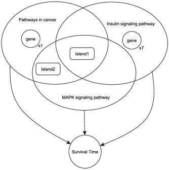
Figure 4: Microarray data: Graphical representation of a subset of selected pathways with islands and singletons. The genes in the islands are listed in Table 1.

In addition, several genes with known association to breast cancer were also selected. Protein kinase C alpha (PKCA), which belongs to the MAPK pathway and the KEGG pathways in cancer, has been reported to play roles in many different cellular processes, including cell functions associated with breast cancer progression. It has been shown to be overexpressed in some antiestrogen resistant breast cancer cell lines and to be involved in the growth of tamoxifen resistant human breast cancer cells [Frankel et al. (2007)]. Patients with PKCA-positive tumors have been shown to have worse survival than patients with PKCA-negative tumors, independently of other factors [Lønne et al. (2010)]. Prostaglandin-endoperoxide synthase-2 (PTGS2, also known as cyclooxygenase-2 or COX2) has also been related to breast cancer. Denkert, Winzer and Hauptmann (2004) observed COX2 overexpression in breast cancer and strong association with indicators of poor prognosis, such as lymph node metastasis, poor differentiation and large tumor size. This was further confirmed by Gupta et al. (2007), who showed that the expression of COX2 in human breast cancer cells facilitates the assembly of new tumor blood vessels, the release of tumor cells into the circulation, and the breaching of lung capillaries by circulating tumor cells to seed pulmonary metastasis. This is an important finding, as the majority of breast cancer deaths result from metastases rather than direct effects of the primary tumor. Another gene previously shown to be predictive of breast cancer lung metastasis is integrin, beta-8 (ITGB8) [Landemaine et al. (2008)]. We also identified integrin, beta-4 (ITGB4) which regulates key signaling pathways related to carcinoma progression, and is linked to aggressive tumor behavior and poor prognosis in certain breast cancer subtypes [Guo et al. (2006)].

5 Discussion

We have proposed a model that incorporates biological knowledge from pathway databases into the analysis of DNA microarrays to identify pathways and genes related to a phenotype. Information on pathway membership and gene networks are used to define pathway summaries, specify prior distributions that account for the dependence structure between genes, and define the MCMC moves to fit the model. The gene network prior and the synthesis of the pathway information through PLS bring in additional information that is especially useful in microarray data, due to the low sample size and large measurement error. Performances of the method were evaluated on simulated data and a breast cancer gene expression study with survival outcomes was used to illustrate its application.

Our simulation studies show the effect of the MRF prior on the posterior inference. In general, as expected, the effect of the prior depends on the data and, in particular, on the concordance of the prior network with the data. In our simulations, employing the MRF prior allows us to achieve a better separation of the relevant pathways from those not relevant (in particular, we have found a larger average difference, over three scenarios, between the relevant pathway with the lowest posterior probability and the nonrelevant pathway with the highest posterior probability). In addition, in the simulated setting with fairly small regression coefficients the model with the MRF prior was able to select all the correct genes without any false positive, while the model without MRF includes 3 false positives. Other authors have reported improvements on selection power and sensitivity with respect to commonly used procedures that do not use the pathway structure, with similar, and in some cases, lower false discovery rates. In addition, in our formulation of the model we have used biological information not only for prior specification but also to structure the MCMC moves. This is helpful in arriving at promising models avoiding visiting invalid configurations. Finally, in real data applications, we have found that employing information on gene–gene networks can lead to the selection of significant genes that would have been missed otherwise, aiding the interpretation of the results, and achieving better predictions compared to models that do not treat genes as connected elements that work in groups or pathways.

Several MRF priors for gene selection indicators have been proposed in the literature. It is interesting to compare the parametrization of the MRF used in this paper and in Li and Zhang (2010) to the parametrization used in Wei and Li (2007, 2008), where the prior on $\bolds\gamma$ is defined as

$$P(\bolds\gamma|\cdot)\propto\exp(dn_{1}-gn_{01}),$$ (19)

where $n_{1}$ is the number of selected genes and $n_{01}$ is the number of edges linking genes with different values of $\gamma_{j}$, that is, edges linking included and nonincluded genes among all pathways,

$$n_{1}=\sum_{j=1}^{p}\gamma_{j},\qquad n_{01}=\frac{1}{2}\sum_{i=1}^{p}\Biggl{[}\sum_{j=1}^{p}r_{ij}-\Biggl{|}\sum_{j=1}^{p}r_{ij}(1-\gamma_{i})-\sum_{j=1}^{p}r_{ij}\gamma_{j}\Biggr{|}\ \Biggr{]}.$$

While $d$ plays the same role as $\mu$ in (12), the parametrization using $g$ has a different effect from $\eta$ on the probability of selection of a gene. This is evident from the conditional probability $P(\gamma_{j}|\cdot,\gamma_{i},i\in N_{j})=\frac{\exp(\gamma_{j}F(\gamma_{j}))}{1+\exp(F(\gamma_{j}))}$, where $F(\gamma_{j})=d+g\sum_{i\in N_{j}}(2\gamma_{i}-1)$. Higher values of $g$ encourage neighboring genes to take on the same $\gamma_{j}$ value, and, consequently, genes with nonselected neighbors have lower prior probability of being selected than genes with no neighbors. We felt that parametrization (12) was a better choice for our purposes. First, in a context of sparsity, where only few nodes are supposed to take value 1, a prior that assigns larger probability of inclusion to genes with selected neighbors than to isolated genes seems more appropriate. Second, the exact simulation algorithm of Propp and Wilson (1996) cannot be used to simulate from (19). While any other method to draw from (19) would be acceptable, as said by Møller et al. (2006), Markov chain methods, to sample from a MRF, require to check at each step that the chain has converged to the equilibrium distribution, to avoid introducing additional undesirable stochasticity. On the other hand, one advantage of parametrization (19) is that no phase transition problem is associated to the distribution.

Pathway databases are incomplete and the gene network information is often unavailable for many genes. Thus, there may be situations where the dependence structure and the MRF prior specification on the gene selection indicator, $\bolds\gamma$, cannot be used for all genes. When the only information available is the pathway membership of genes, the prior on $\bolds\gamma$ could be elicited to capture other interesting characteristics. For example, a gene can have a priori higher probability of being selected when several pathways that contain it are included in the model. We may also want to avoid favoring the selection of a large pathway just because of its size. In such cases, conditional on $\bolds\theta$, independent Bernoulli priors can be specified for $\gamma_{j}$ relating the probability of selection to the proportion of included pathways that contain gene $j$, adjusting for the pathway sizes, $p_{k}$, that is, $\gamma_{j}|\bolds\theta\sim\operatorname{Bernoulli}(c\cdot\frac{\sum_{k=1}^{K}\theta_{k}s_{kj}/p_{k}}{\sum_{k=1}^{K}s_{kj}/p_{k}})$, with $c$ a hyperparameter to be elicited.

In our approach we have made use of PLS components as summary measures of the expression of genes belonging to known pathways and then applied a fully Bayesian approach for the selection of the pathways to be included in the model, and the genes to be included within those pathways. Penalized techniques, including lasso [Tibshirani (1996)], elastic net [Zou and Hastie (2005)] and group lasso [Yuan and Lin (2006)] have been studied extensively in the literature and have been successfully applied to gene expression data. The group lasso, in particular, defines sets of variables, then selects either all the variables in the group or none of them. Recently, a modification of the method was proposed by Friedman, Hastie and Tibshirani (2010) using a more general penalty that yields sparsity at both the group and individual feature levels to select groups and predictors within each group. Our understanding of group lasso is that the method works best in situations where variables belonging to the same group are highly correlated, while covariates in different groups do not exhibit high correlation. However, genes belonging to the same pathway often do not exhibit high correlation in their expression levels. Also, in our case there are genes belonging to different pathways that have high correlation, as well as genes that belong to more than one pathway. Initial investigations suggest that, in terms of prediction MSE, Bayesian formulations of lasso methods perform similarly to and, in some cases, better than the frequentist lasso [see, e.g., Kyung et al. (2010)]. Particularly relevant to our approach is the work of Guan and Stephens (2011), who apply Bayesian variable selection (BVS) and stochastic search methods in a regression model for genome-wide data. In simulations they find that, in spite of the apparent computational challenges, BVS produces better power and predictive performance compared with standard lasso techniques.

Supplement [doi]10.1214/11-AOAS463SUPP [url]http://lib.stat.cmu.edu/aoas/463/supplement.pdf .pdf Description of the MCMC steps for $(\bolds\theta,\bolds\gamma)$ and discussion on ergodicity of the Markov chain on the restricted space.

References

- Albert and Chib (1993) {barticle}[mr] \bauthor\bsnmAlbert, \bfnmJames H.\binitsJ. H. and \bauthor\bsnmChib, \bfnmSiddhartha\binitsS. (\byear1993). \btitleBayesian analysis of binary and polychotomous response data. \bjournalJ. Amer. Statist. Assoc. \bvolume88 \bpages669–679. \bidissn=0162-1459, mr=1224394 \endbibitem
- Ashburner et al. (2000) {barticle}[pbm] \bauthor\bsnmAshburner, \bfnmM.\binitsM., \bauthor\bsnmBall, \bfnmC. A.\binitsC. A., \bauthor\bsnmBlake, \bfnmJ. A.\binitsJ. A., \bauthor\bsnmBotstein, \bfnmD.\binitsD., \bauthor\bsnmButler, \bfnmH.\binitsH., \bauthor\bsnmCherry, \bfnmJ. M.\binitsJ. M., \bauthor\bsnmDavis, \bfnmA. P.\binitsA. P., \bauthor\bsnmDolinski, \bfnmK.\binitsK., \bauthor\bsnmDwight, \bfnmS. S.\binitsS. S., \bauthor\bsnmEppig, \bfnmJ. T.\binitsJ. T., \bauthor\bsnmHarris, \bfnmM. A.\binitsM. A., \bauthor\bsnmHill, \bfnmD. P.\binitsD. P., \bauthor\bsnmIssel-Tarver, \bfnmL.\binitsL., \bauthor\bsnmKasarskis, \bfnmA.\binitsA., \bauthor\bsnmLewis, \bfnmS.\binitsS., \bauthor\bsnmMatese, \bfnmJ. C.\binitsJ. C., \bauthor\bsnmRichardson, \bfnmJ. E.\binitsJ. E., \bauthor\bsnmRingwald, \bfnmM.\binitsM., \bauthor\bsnmRubin, \bfnmG. M.\binitsG. M. and \bauthor\bsnmSherlock, \bfnmG.\binitsG. (\byear2000). \btitleGene ontology: Tool for the unification of biology. The Gene Ontology Consortium. \bjournalNat. Genet. \bvolume25 \bpages25–29. \biddoi=10.1038/75556, issn=1061-4036, mid=NIHMS269796, pmcid=3037419, pmid=10802651 \endbibitem
- Bair et al. (2006) {barticle}[mr] \bauthor\bsnmBair, \bfnmEric\binitsE., \bauthor\bsnmHastie, \bfnmTrevor\binitsT., \bauthor\bsnmPaul, \bfnmDebashis\binitsD. and \bauthor\bsnmTibshirani, \bfnmRobert\binitsR. (\byear2006). \btitlePrediction by supervised principal components. \bjournalJ. Amer. Statist. Assoc. \bvolume101 \bpages119–137. \biddoi=10.1198/016214505000000628, issn=0162-1459, mr=2252436 \endbibitem
- Besag (1974) {barticle}[mr] \bauthor\bsnmBesag, \bfnmJulian\binitsJ. (\byear1974). \btitleSpatial interaction and the statistical analysis of lattice systems. \bjournalJ. Roy. Statist. Soc. Ser. B \bvolume36 \bpages192–236. \bidissn=0035-9246, mr=0373208 \endbibitem
- Bild et al. (2006) {barticle}[pbm] \bauthor\bsnmBild, \bfnmAndrea H.\binitsA. H., \bauthor\bsnmYao, \bfnmGuang\binitsG., \bauthor\bsnmChang, \bfnmJeffrey T.\binitsJ. T., \bauthor\bsnmWang, \bfnmQuanli\binitsQ., \bauthor\bsnmPotti, \bfnmAnil\binitsA., \bauthor\bsnmChasse, \bfnmDawn\binitsD., \bauthor\bsnmJoshi, \bfnmMary-Beth\binitsM.-B., \bauthor\bsnmHarpole, \bfnmDavid\binitsD., \bauthor\bsnmLancaster, \bfnmJohnathan M.\binitsJ. M., \bauthor\bsnmBerchuck, \bfnmAndrew\binitsA., \bauthor\bsnmOlson, \bfnmJohn A.\binitsJ. A. Jr., \bauthor\bsnmMarks, \bfnmJeffrey R.\binitsJ. R., \bauthor\bsnmDressman, \bfnmHolly K.\binitsH. K., \bauthor\bsnmWest, \bfnmMike\binitsM. and \bauthor\bsnmNevins, \bfnmJoseph R.\binitsJ. R. (\byear2006). \btitleOncogenic pathway signatures in human cancers as a guide to targeted therapies. \bjournalNature \bvolume439 \bpages353–357. \biddoi=10.1038/nature04296, issn=1476-4687, pii=nature04296, pmid=16273092 \endbibitem
- Boulesteix and Strimmer (2007) {barticle}[pbm] \bauthor\bsnmBoulesteix, \bfnmAnne-Laure\binitsA.-L. and \bauthor\bsnmStrimmer, \bfnmKorbinian\binitsK. (\byear2007). \btitlePartial least squares: A versatile tool for the analysis of high-dimensional genomic data. \bjournalBrief. Bioinformatics \bvolume8 \bpages32–44. \biddoi=10.1093/bib/bbl016, issn=1467-5463, pii=bbl016, pmid=16772269 \endbibitem
- Brown, Vannucci and Fearn (1998) {barticle}[mr] \bauthor\bsnmBrown, \bfnmP. J.\binitsP. J., \bauthor\bsnmVannucci, \bfnmM.\binitsM. and \bauthor\bsnmFearn, \bfnmT.\binitsT. (\byear1998). \btitleMultivariate Bayesian variable selection and prediction. \bjournalJ. R. Stat. Soc. Ser. B Stat. Methodol. \bvolume60 \bpages627–641. \biddoi=10.1111/1467-9868.00144, issn=1369-7412, mr=1626005 \endbibitem
- Chipman, George and McCulloch (2001) {bincollection}[mr] \bauthor\bsnmChipman, \bfnmHugh\binitsH., \bauthor\bsnmGeorge, \bfnmEdward I.\binitsE. I. and \bauthor\bsnmMcCulloch, \bfnmRobert E.\binitsR. E. (\byear2001). \btitleThe practical implementation of Bayesian model selection. In \bbooktitleModel Selection. \bseriesInstitute of Mathematical Statistics Lecture Notes—Monograph Series \bvolume38 \bpages65–134. \bpublisherIMS, \baddressBeachwood, OH. \biddoi=10.1214/lnms/1215540964, mr=2000752 \endbibitem
- Dahlquist et al. (2002) {barticle}[pbm] \bauthor\bsnmDahlquist, \bfnmKam D.\binitsK. D., \bauthor\bsnmSalomonis, \bfnmNathan\binitsN., \bauthor\bsnmVranizan, \bfnmKaren\binitsK., \bauthor\bsnmLawlor, \bfnmSteven C.\binitsS. C. and \bauthor\bsnmConklin, \bfnmBruce R.\binitsB. R. (\byear2002). \btitleGenMAPP, a new tool for viewing and analyzing microarray data on biological pathways. \bjournalNat. Genet. \bvolume31 \bpages19–20. \biddoi=10.1038/ng0502-19, issn=1061-4036, pii=ng0502-19, pmid=11984561 \endbibitem
- Denkert, Winzer and Hauptmann (2004) {barticle}[pbm] \bauthor\bsnmDenkert, \bfnmCarsten\binitsC., \bauthor\bsnmWinzer, \bfnmKlaus-Jürgen\binitsK.-J. and \bauthor\bsnmHauptmann, \bfnmSteffen\binitsS. (\byear2004). \btitlePrognostic impact of cyclooxygenase-2 in breast cancer. \bjournalClin. Breast Cancer \bvolume4 \bpages428–433. \bidissn=1526-8209, pmid=15023244 \endbibitem
- Doniger et al. (2003) {barticle}[auto:STB—2011-03-03—12:04:44] \bauthor\bsnmDoniger, \bfnmS.\binitsS., \bauthor\bsnmSalomonis, \bfnmN.\binitsN., \bauthor\bsnmDahlquist, \bfnmK.\binitsK., \bauthor\bsnmVranizan, \bfnmK.\binitsK., \bauthor\bsnmLawlor, \bfnmS.\binitsS. and \bauthor\bsnmConklin, \bfnmB.\binitsB. (\byear2003). \btitleMAPPFinder: Using Gene Ontology and GenMAPP to create a global gene-expression profile for microarray data. \bjournalGenome Biology \bvolume41 \bpagesR7. \endbibitem
- Downward (2006) {barticle}[pbm] \bauthor\bsnmDownward, \bfnmJulian\binitsJ. (\byear2006). \btitleCancer biology: Signatures guide drug choice. \bjournalNature \bvolume439 \bpages274–275. \biddoi=10.1038/439274a, issn=1476-4687, pii=439274a, pmid=16421553 \endbibitem
- Frankel et al. (2007) {barticle}[pbm] \bauthor\bsnmFrankel, \bfnmLisa B.\binitsL. B., \bauthor\bsnmLykkesfeldt, \bfnmAnne E.\binitsA. E., \bauthor\bsnmHansen, \bfnmJens B.\binitsJ. B. and \bauthor\bsnmStenvang, \bfnmJan\binitsJ. (\byear2007). \btitleProtein Kinase C alpha is a marker for antiestrogen resistance and is involved in the growth of tamoxifen resistant human breast cancer cells. \bjournalBreast Cancer Res. Treat. \bvolume104 \bpages165–179. \biddoi=10.1007/s10549-006-9399-1, issn=0167-6806, pmid=17061041 \endbibitem
- Friedman, Hastie and Tibshirani (2010) {bmisc}[auto:STB—2011-03-03—12:04:44] \bauthor\bsnmFriedman, \bfnmJ.\binitsJ., \bauthor\bsnmHastie, \bfnmT.\binitsT. and \bauthor\bsnmTibshirani, \bfnmR.\binitsR. (\byear2010). \bhowpublishedA note on the group lasso and a sparse group lasso. Technical report, Dept. Stat., Stanford Univ. \endbibitem
- George and McCulloch (1997) {barticle}[auto:STB—2011-03-03—12:04:44] \bauthor\bsnmGeorge, \bfnmE. I.\binitsE. I. and \bauthor\bsnmMcCulloch, \bfnmR. E.\binitsR. E. (\byear1997). \btitleApproaches for Bayesian variable selection. \bjournalStatist. Sinica \bvolume7 \bpages339–373. \endbibitem
- Golub et al. (1999) {barticle}[auto:STB—2011-03-03—12:04:44] \bauthor\bsnmGolub, \bfnmT. R.\binitsT. R., \bauthor\bsnmSlonim, \bfnmD. K.\binitsD. K., \bauthor\bsnmTamayo, \bfnmP.\binitsP., \bauthor\bsnmHuard, \bfnmC.\binitsC., \bauthor\bsnmGaasenbeek, \bfnmM.\binitsM., \bauthor\bsnmMesirov, \bfnmJ. P.\binitsJ. P., \bauthor\bsnmColler, \bfnmH.\binitsH., \bauthor\bsnmLoh, \bfnmM. L.\binitsM. L., \bauthor\bsnmDowning, \bfnmJ. R.\binitsJ. R., \bauthor\bsnmCaligiuri, \bfnmM. A.\binitsM. A., \bauthor\bsnmBloomfield, \bfnmC. D.\binitsC. D. and \bauthor\bsnmLander, \bfnmE.\binitsE. (\byear1999). \btitleMolecular classification of cancer: Class discovery and class prediction by gene expression monitoring. \bjournalScience \bvolume286 \bpages531–537. \endbibitem
- Guan and Stephens (2011) {bmisc}[auto:STB—2011-03-03—12:04:44] \bauthor\bsnmGuan, \bfnmY.\binitsY. and \bauthor\bsnmStephens, \bfnmM.\binitsM. (\byear2011). \bhowpublishedBayesian variable selection regression for genome-wide association studies, and other large-scale problems. Ann. Appl. Stat. To appear. \endbibitem
- Guo et al. (2006) {barticle}[pbm] \bauthor\bsnmGuo, \bfnmWenjun\binitsW., \bauthor\bsnmPylayeva, \bfnmYuliya\binitsY., \bauthor\bsnmPepe, \bfnmAngela\binitsA., \bauthor\bsnmYoshioka, \bfnmToshiaki\binitsT., \bauthor\bsnmMuller, \bfnmWilliam J.\binitsW. J., \bauthor\bsnmInghirami, \bfnmGiorgio\binitsG. and \bauthor\bsnmGiancotti, \bfnmFilippo G.\binitsF. G. (\byear2006). \btitleBeta 4 integrin amplifies ErbB2 signaling to promote mammary tumorigenesis. \bjournalCell \bvolume126 \bpages489–502. \biddoi=10.1016/j.cell.2006.05.047, issn=0092-8674, pii=S0092-8674(06)00907-X, pmid=16901783 \endbibitem
- Gupta et al. (2007) {barticle}[pbm] \bauthor\bsnmGupta, \bfnmGaorav P.\binitsG. P., \bauthor\bsnmNguyen, \bfnmDon X.\binitsD. X., \bauthor\bsnmChiang, \bfnmAnne C.\binitsA. C., \bauthor\bsnmBos, \bfnmPaula D.\binitsP. D., \bauthor\bsnmKim, \bfnmJuliet Y.\binitsJ. Y., \bauthor\bsnmNadal, \bfnmCristina\binitsC., \bauthor\bsnmGomis, \bfnmRoger R.\binitsR. R., \bauthor\bsnmManova-Todorova, \bfnmKatia\binitsK. and \bauthor\bsnmMassagué, \bfnmJoan\binitsJ. (\byear2007). \btitleMediators of vascular remodelling co-opted for sequential steps in lung metastasis. \bjournalNature \bvolume446 \bpages765–770. \biddoi=10.1038/nature05760, issn=1476-4687, pii=nature05760, pmid=17429393 \endbibitem
- Joshi-Tope et al. (2005) {barticle}[pbm] \bauthor\bsnmJoshi-Tope, \bfnmG.\binitsG., \bauthor\bsnmGillespie, \bfnmM.\binitsM., \bauthor\bsnmVastrik, \bfnmI.\binitsI., \bauthor\bsnmD’Eustachio, \bfnmP.\binitsP., \bauthor\bsnmSchmidt, \bfnmE.\binitsE., \bauthor\bparticlede \bsnmBono, \bfnmB.\binitsB., \bauthor\bsnmJassal, \bfnmB.\binitsB., \bauthor\bsnmGopinath, \bfnmG. R.\binitsG. R., \bauthor\bsnmWu, \bfnmG. R.\binitsG. R., \bauthor\bsnmMatthews, \bfnmL.\binitsL., \bauthor\bsnmLewis, \bfnmS.\binitsS., \bauthor\bsnmBirney, \bfnmE.\binitsE. and \bauthor\bsnmStein, \bfnmL.\binitsL. (\byear2005). \btitleReactome: A knowledgebase of biological pathways. \bjournalNucleic Acids Res. \bvolume33 \bpagesD428–D432. \biddoi=10.1093/nar/gki072, issn=1362-4962, pii=33/suppl_1/D428, pmcid=540026, pmid=15608231 \endbibitem
- Kanehisa and Goto (2000) {barticle}[auto:STB—2011-03-03—12:04:44] \bauthor\bsnmKanehisa, \bfnmM.\binitsM. and \bauthor\bsnmGoto, \bfnmS.\binitsS. (\byear2000). \btitleKyoto encyclopedia of genes and genomes. \bjournalNucleic Acids Res. \bvolume28 \bpages27–30. \endbibitem
- Krieger et al. (2004) {barticle}[auto:STB—2011-03-03—12:04:44] \bauthor\bsnmKrieger, \bfnmC.\binitsC., \bauthor\bsnmZhang, \bfnmP.\binitsP., \bauthor\bsnmMueller, \bfnmL.\binitsL., \bauthor\bsnmWang, \bfnmA.\binitsA., \bauthor\bsnmPaley, \bfnmS.\binitsS., \bauthor\bsnmArnaud, \bfnmM.\binitsM., \bauthor\bsnmPick, \bfnmJ.\binitsJ., \bauthor\bsnmRhee, \bfnmS.\binitsS. and \bauthor\bsnmKarp, \bfnmP.\binitsP. (\byear2004). \btitleMetaCyc: A multiorganism database of metabolic pathways and enzymes. \bjournalNucleic Acids Res. \bvolume32 \bpagesD438–442. \endbibitem
- Kwon et al. (2007) {barticle}[pbm] \bauthor\bsnmKwon, \bfnmDeukwoo\binitsD., \bauthor\bsnmTadesse, \bfnmMahlet G.\binitsM. G., \bauthor\bsnmSha, \bfnmNaijun\binitsN., \bauthor\bsnmPfeiffer, \bfnmRuth M.\binitsR. M. and \bauthor\bsnmVannucci, \bfnmMarina\binitsM. (\byear2007). \btitleIdentifying biomarkers from mass spectrometry data with ordinal outcome. \bjournalCancer Inform. \bvolume3 \bpages19–28. \bidissn=1176-9351, pmcid=2675849, pmid=19455232 \endbibitem
- Kyung et al. (2010) {barticle}[auto:STB—2011-03-03—12:04:44] \bauthor\bsnmKyung, \bfnmM.\binitsM., \bauthor\bsnmGill, \bfnmJ.\binitsJ., \bauthor\bsnmGhosh, \bfnmM.\binitsM. and \bauthor\bsnmCasella, \bfnmG.\binitsG. (\byear2010). \btitlePenalized regression, standard errors, and Bayesian lassos. \bjournalBayesian Anal. \bvolume5 \bpages369–412. \endbibitem
- Landemaine et al. (2008) {barticle}[pbm] \bauthor\bsnmLandemaine, \bfnmThomas\binitsT., \bauthor\bsnmJackson, \bfnmAmanda\binitsA., \bauthor\bsnmBellahcène, \bfnmAkeila\binitsA., \bauthor\bsnmRucci, \bfnmNadia\binitsN., \bauthor\bsnmSin, \bfnmSoraya\binitsS., \bauthor\bsnmAbad, \bfnmBerta Martin\binitsB. M., \bauthor\bsnmSierra, \bfnmAngels\binitsA., \bauthor\bsnmBoudinet, \bfnmAlain\binitsA., \bauthor\bsnmGuinebretière, \bfnmJean-Marc\binitsJ.-M., \bauthor\bsnmRicevuto, \bfnmEnrico\binitsE., \bauthor\bsnmNoguès, \bfnmCatherine\binitsC., \bauthor\bsnmBriffod, \bfnmMarianne\binitsM., \bauthor\bsnmBièche, \bfnmIvan\binitsI., \bauthor\bsnmCherel, \bfnmPascal\binitsP., \bauthor\bsnmGarcia, \bfnmTeresa\binitsT., \bauthor\bsnmCastronovo, \bfnmVincent\binitsV., \bauthor\bsnmTeti, \bfnmAnna\binitsA., \bauthor\bsnmLidereau, \bfnmRosette\binitsR. and \bauthor\bsnmDriouch, \bfnmKeltouma\binitsK. (\byear2008). \btitleA six-gene signature predicting breast cancer lung metastasis. \bjournalCancer Res. \bvolume68 \bpages6092–6099. \biddoi=10.1158/0008-5472.CAN-08-0436, issn=1538-7445, pii=68/15/6092, pmid=18676831 \endbibitem
- Lee et al. (2007) {barticle}[auto:STB—2011-03-03—12:04:44] \bauthor\bsnmLee, \bfnmS.\binitsS., \bauthor\bsnmJeong, \bfnmY.\binitsY., \bauthor\bsnmIm, \bfnmH. G.\binitsH. G., \bauthor\bsnmKim, \bfnmC.\binitsC., \bauthor\bsnmChang, \bfnmY.\binitsY. and \bauthor\bsnmLee, \bfnmI.\binitsI. (\byear2007). \btitleSilibinin suppresses PMA-induced MMP-9 expression by blocking the AP-1 activation via MAPK signaling pathways in MCF-7 human breast carcinoma cells. \bjournalBiochemical and Biophysical Research Communications \bvolume354 \bpages65–171. \endbibitem
- Li and Li (2008) {barticle}[auto:STB—2011-03-03—12:04:44] \bauthor\bsnmLi, \bfnmC.\binitsC. and \bauthor\bsnmLi, \bfnmH.\binitsH. (\byear2008). \btitleNetwork-constrained regularization and variable selection for analysis of genomics data. \bjournalBioinformatics \bvolume24 \bpages1175–1182. \endbibitem
- Li and Zhang (2010) {barticle}[auto:STB—2011-03-03—12:04:44] \bauthor\bsnmLi, \bfnmF.\binitsF. and \bauthor\bsnmZhang, \bfnmN.\binitsN. (\byear2010). \btitleBayesian Variable selection in structured high-dimensional covariate space with application in genomics. \bjournalJ. Amer. Statist. Assoc. \bvolume105 \bpages1202–1214. \endbibitem
- Lindgren, Geladi and Wold (1993) {barticle}[auto:STB—2011-03-03—12:04:44] \bauthor\bsnmLindgren, \bfnmF.\binitsF., \bauthor\bsnmGeladi, \bfnmP.\binitsP. and \bauthor\bsnmWold, \bfnmS.\binitsS. (\byear1993). \btitleThe kernel algorithm of PLS. \bjournalJournal of Chemometrics \bvolume7 \bpages45–59. \endbibitem
- Lønne et al. (2010) {barticle}[pbm] \bauthor\bsnmLønne, \bfnmGry Kalstad\binitsG. K., \bauthor\bsnmCornmark, \bfnmLouise\binitsL., \bauthor\bsnmZahirovic, \bfnmIris Omanovic\binitsI. O., \bauthor\bsnmLandberg, \bfnmGöran\binitsG., \bauthor\bsnmJirström, \bfnmKarin\binitsK. and \bauthor\bsnmLarsson, \bfnmChrister\binitsC. (\byear2010). \btitlePKCalpha expression is a marker for breast cancer aggressiveness. \bjournalMol. Cancer \bvolume9 \bpages76. \biddoi=10.1186/1476-4598-9-76, issn=1476-4598, pii=1476-4598-9-76, pmcid=2873434, pmid=20398285 \endbibitem
- Lucas, Carvalho, Wang, Bild, Nevins and West (2006) {bincollection}[auto:STB—2011-03-03—12:04:44] \beditor\bsnmLucas, \bfnmJ.\binitsJ., \bauthor\bsnmCarvalho, \bfnmC.\binitsC., \bauthor\bsnmWang, \bfnmQ.\binitsQ., \bauthor\bsnmBild, \bfnmA.\binitsA. \beditor\bsnmNevins, \bfnmJ.\binitsJ. and \beditor\bsnmWest, \bfnmM.\binitsM. (\byear2006). \btitleSparse statistical modelling in gene expression genomics. In \bbooktitleBayesian Inference for Gene Expression and Proteomics (\beditorK. Do, \beditorP. Mueller and \beditorM. Vannucci, eds.) \bpages155–176. \bpublisherCambridge Univ. Press, \baddressCambridge. \endbibitem
- Møller et al. (2006) {barticle}[mr] \bauthor\bsnmMøller, \bfnmJ.\binitsJ., \bauthor\bsnmPettitt, \bfnmA. N.\binitsA. N., \bauthor\bsnmReeves, \bfnmR.\binitsR. and \bauthor\bsnmBerthelsen, \bfnmK. K.\binitsK. K. (\byear2006). \btitleAn efficient Markov chain Monte Carlo method for distributions with intractable normalising constants. \bjournalBiometrika \bvolume93 \bpages451–458. \biddoi=10.1093/biomet/93.2.451, issn=0006-3444, mr=2278096 \endbibitem
- Nakao et al. (1999) {barticle}[auto:STB—2011-03-03—12:04:44] \bauthor\bsnmNakao, \bfnmM.\binitsM., \bauthor\bsnmBono, \bfnmH.\binitsH., \bauthor\bsnmKawashima, \bfnmS.\binitsS., \bauthor\bsnmKamiya, \bfnmT.\binitsT., \bauthor\bsnmSato, \bfnmK.\binitsK., \bauthor\bsnmGoto, \bfnmS.\binitsS. and \bauthor\bsnmKanehisa, \bfnmM.\binitsM. (\byear1999). \btitleGenome-scale gene expression analysis and pathway reconstruction in KEGG. \bjournalGenome Informatics Series: Workshop on Genome Informatics \bvolume10 \bpages94–103. \endbibitem
- Pan, Xie and Shen (2010) {barticle}[mr] \bauthor\bsnmPan, \bfnmWei\binitsW., \bauthor\bsnmXie, \bfnmBenhuai\binitsB. and \bauthor\bsnmShen, \bfnmXiaotong\binitsX. (\byear2010). \btitleIncorporating predictor network in penalized regression with application to microarray data. \bjournalBiometrics \bvolume66 \bpages474–484. \endbibitem
- Park, Hastie and Tibshirani (2007) {barticle}[pbm] \bauthor\bsnmPark, \bfnmMee Young\binitsM. Y., \bauthor\bsnmHastie, \bfnmTrevor\binitsT. and \bauthor\bsnmTibshirani, \bfnmRobert\binitsR. (\byear2007). \btitleAveraged gene expressions for regression. \bjournalBiostatistics \bvolume8 \bpages212–227. \biddoi=10.1093/biostatistics/kxl002, issn=1465-4644, pii=kxl002, pmid=16698769 \endbibitem
- Pittman et al. (2004) {barticle}[auto:STB—2011-03-03—12:04:44] \bauthor\bsnmPittman, \bfnmJ.\binitsJ., \bauthor\bsnmHuang, \bfnmE.\binitsE., \bauthor\bsnmDressman, \bfnmH.\binitsH., \bauthor\bsnmHorng, \bfnmC.\binitsC., \bauthor\bsnmCheng, \bfnmS.\binitsS., \bauthor\bsnmTsou, \bfnmM.\binitsM., \bauthor\bsnmChen, \bfnmC.\binitsC., \bauthor\bsnmBild, \bfnmA.\binitsA., \bauthor\bsnmIversen, \bfnmE.\binitsE., \bauthor\bsnmHuang, \bfnmA.\binitsA., \bauthor\bsnmNevins, \bfnmJ.\binitsJ. and \bauthor\bsnmWest, \bfnmM.\binitsM. (\byear2004). \btitleIntegrated modeling of clinical and gene expression information for personalized prediction of disease outcomes. \bjournalProc. Natl. Acad. Sci. USA \bvolume101 \bpages8431–8436. \endbibitem
- Propp and Wilson (1996) {binproceedings}[mr] \bauthor\bsnmPropp, \bfnmJames Gary\binitsJ. G. and \bauthor\bsnmWilson, \bfnmDavid Bruce\binitsD. B. (\byear1996). \btitleExact sampling with coupled Markov chains and applications to statistical mechanics. In \bbooktitleProceedings of the Seventh International Conference on Random Structures and Algorithms (Atlanta, GA, 1995) \bvolume9 \bpages223–252. \biddoi=10.1002/(SICI)1098-2418(199608/09)9:1/2<223::AID-RSA14>3.3.CO; 2-R, issn=1042-9832, mr=1611693 \endbibitem
- Sha, Tadesse and Vannucci (2006) {barticle}[pbm] \bauthor\bsnmSha, \bfnmNaijun\binitsN., \bauthor\bsnmTadesse, \bfnmMahlet G.\binitsM. G. and \bauthor\bsnmVannucci, \bfnmMarina\binitsM. (\byear2006). \btitleBayesian variable selection for the analysis of microarray data with censored outcomes. \bjournalBioinformatics \bvolume22 \bpages2262–2268. \biddoi=10.1093/bioinformatics/btl362, issn=1367-4811, pii=btl362, pmid=16845144 \endbibitem
- Sha et al. (2004) {barticle}[mr] \bauthor\bsnmSha, \bfnmNaijun\binitsN., \bauthor\bsnmVannucci, \bfnmMarina\binitsM., \bauthor\bsnmTadesse, \bfnmMahlet G.\binitsM. G., \bauthor\bsnmBrown, \bfnmPhilip J.\binitsP. J., \bauthor\bsnmDragoni, \bfnmIlaria\binitsI., \bauthor\bsnmDavies, \bfnmNick\binitsN., \bauthor\bsnmRoberts, \bfnmTracy C.\binitsT. C., \bauthor\bsnmContestabile, \bfnmAndrea\binitsA., \bauthor\bsnmSalmon, \bfnmMike\binitsM., \bauthor\bsnmBuckley, \bfnmChris\binitsC. and \bauthor\bsnmFalciani, \bfnmFancesco\binitsF. (\byear2004). \btitleBayesian variable selection in multinomial probit models to identify molecular signatures of disease stage. \bjournalBiometrics \bvolume60 \bpages812–828. \biddoi=10.1111/j.0006-341X.2004.00233.x, issn=0006-341X, mr=2089459 \endbibitem
- Shipp et al. (2002) {barticle}[pbm] \bauthor\bsnmShipp, \bfnmMargaret A.\binitsM. A., \bauthor\bsnmRoss, \bfnmKen N.\binitsK. N., \bauthor\bsnmTamayo, \bfnmPablo\binitsP., \bauthor\bsnmWeng, \bfnmAndrew P.\binitsA. P., \bauthor\bsnmKutok, \bfnmJeffery L.\binitsJ. L., \bauthor\bsnmAguiar, \bfnmRicardo C T\binitsR. C. T., \bauthor\bsnmGaasenbeek, \bfnmMichelle\binitsM., \bauthor\bsnmAngelo, \bfnmMichael\binitsM., \bauthor\bsnmReich, \bfnmMichael\binitsM., \bauthor\bsnmPinkus, \bfnmGeraldine S.\binitsG. S., \bauthor\bsnmRay, \bfnmTane S.\binitsT. S., \bauthor\bsnmKoval, \bfnmMargaret A.\binitsM. A., \bauthor\bsnmLast, \bfnmKim W.\binitsK. W., \bauthor\bsnmNorton, \bfnmAndrew\binitsA., \bauthor\bsnmLister, \bfnmT. Andrew\binitsT. A., \bauthor\bsnmMesirov, \bfnmJill\binitsJ., \bauthor\bsnmNeuberg, \bfnmDonna S.\binitsD. S., \bauthor\bsnmLander, \bfnmEric S.\binitsE. S., \bauthor\bsnmAster, \bfnmJon C.\binitsJ. C. and \bauthor\bsnmGolub, \bfnmTodd R.\binitsT. R. (\byear2002). \btitleDiffuse large B-cell lymphoma outcome prediction by gene-expression profiling and supervised machine learning. \bjournalNat. Med. \bvolume8 \bpages68–74. \biddoi=10.1038/nm0102-68, issn=1078-8956, pii=nm0102-68, pmid=11786909 \endbibitem
- Stingo and Vannucci (2011) {barticle}[auto:STB—2011-03-03—12:04:44] \bauthor\bsnmStingo, \bfnmF.\binitsF. and \bauthor\bsnmVannucci, \bfnmM.\binitsM. (\byear2011). btitleVariable selection for discriminant analysis with Markov random field priors for the analysis of microarray data. \bjournalBioinformatics \bvolume27 \bpages495–501. \endbibitem
- Stingo et al. (2011) {bmisc}[auto:STB—2011-03-03—12:04:44] \bauthor\bsnmStingo, \bfnmF.\binitsF., \bauthor\bsnmChen, \bfnmY.\binitsY., \bauthor\bsnmTadesse, \bfnmM.\binitsM. and \bauthor\bsnmVannucci, \bfnmM.\binitsM. (\byear2011). \bhowpublishedSupplement to: “Incorporating biological information into linear models: A Bayesian approach to the selection of pathways and genes.” DOI:10.1214/11-AOAS463SUPP. \endbibitem
- Subramanian et al. (2005) {barticle}[auto:STB—2011-03-03—12:04:44] \bauthor\bsnmSubramanian, \bfnmA.\binitsA., \bauthor\bsnmTamayo, \bfnmP.\binitsP., \bauthor\bsnmMootha, \bfnmV. K.\binitsV. K., \bauthor\bsnmMukherjee, \bfnmS.\binitsS., \bauthor\bsnmEbert, \bfnmB. L.\binitsB. L., \bauthor\bsnmGillette, \bfnmM. A.\binitsM. A., \bauthor\bsnmPaulovich, \bfnmA.\binitsA., \bauthor\bsnmPomeroy, \bfnmS. L.\binitsS. L., \bauthor\bsnmGolub, \bfnmT. R.\binitsT. R., \bauthor\bsnmLander, \bfnmE. S.\binitsE. S. and \bauthor\bsnmMesirov, \bfnmJ. P.\binitsJ. P. (\byear2005). \btitleGene set enrichment analysis: A knowledge-based approach for interpreting genome-wide expression profiles. \bjournalProc. Natl. Acad. Sci. USA \bvolume102 \bpages15545–15550. \endbibitem
- Telesca et al. (2008) {bmisc}[auto:STB—2011-03-03—12:04:44] \bauthor\bsnmTelesca, \bfnmD.\binitsD., \bauthor\bsnmMuller, \bfnmP.\binitsP., \bauthor\bsnmParmigiani, \bfnmG.\binitsG. and \bauthor\bsnmFreedman, \bfnmR.\binitsR. (\byear2008). \bhowpublishedModeling dependent gene expression. Technical report, Dept. of Biostatistics, Univ. Texas M.D. Anderson Cancer Center. \endbibitem
- Tibshirani (1996) {barticle}[mr] \bauthor\bsnmTibshirani, \bfnmRobert\binitsR. (\byear1996). \btitleRegression shrinkage and selection via the lasso. \bjournalJ. Roy. Statist. Soc. Ser. B \bvolume58 \bpages267–288. \bidissn=0035-9246, mr=1379242 \endbibitem
- Troyanskaya et al. (2001) {barticle}[pbm] \bauthor\bsnmTroyanskaya, \bfnmO.\binitsO., \bauthor\bsnmCantor, \bfnmM.\binitsM., \bauthor\bsnmSherlock, \bfnmG.\binitsG., \bauthor\bsnmBrown, \bfnmP.\binitsP., \bauthor\bsnmHastie, \bfnmT.\binitsT., \bauthor\bsnmTibshirani, \bfnmR.\binitsR., \bauthor\bsnmBotstein, \bfnmD.\binitsD. and \bauthor\bsnmAltman, \bfnmR. B.\binitsR. B. (\byear2001). \btitleMissing value estimation methods for DNA microarrays. \bjournalBioinformatics \bvolume17 \bpages520–525. \bidissn=1367-4803, pmid=11395428 \endbibitem
- van’t Veer et al. (2002) {barticle}[auto:STB—2011-03-03—12:04:44] \bauthor\bparticlevan’t \bsnmVeer, \bfnmL.\binitsL., \bauthor\bsnmDai, \bfnmH.\binitsH., \bauthor\bparticlevan de \bsnmVijver, \bfnmM.\binitsM., \bauthor\bsnmHe, \bfnmY.\binitsY., \bauthor\bsnmHart, \bfnmA.\binitsA., \bauthor\bsnmMao, \bfnmM.\binitsM., \bauthor\bsnmPeterse, \bfnmH.\binitsH., \bauthor\bparticlevan der \bsnmKooy, \bfnmK.\binitsK., \bauthor\bsnmMarton, \bfnmM.\binitsM., \bauthor\bsnmWitteveen, \bfnmA.\binitsA., \bauthor\bsnmSchreiber, \bfnmG.\binitsG., \bauthor\bsnmKerkhoven, \bfnmR.\binitsR., \bauthor\bsnmRoberts, \bfnmC.\binitsC., \bauthor\bsnmLinsley, \bfnmP.\binitsP., \bauthor\bsnmBernards, \bfnmR.\binitsR. and \bauthor\bsnmFriend, \bfnmS.\binitsS. (\byear2002). \btitleGene expression profiling predicts clinical outcome of breast cancer. \bjournalNature \bvolume415 \bpages530–536. \endbibitem
- Wei (1992) {barticle}[pbm] \bauthor\bsnmWei, \bfnmL. J.\binitsL. J. (\byear1992). \btitleThe accelerated failure time model: A useful alternative to the Cox regression model in survival analysis. \bjournalStat. Med. \bvolume11 \bpages1871–1879. \bidissn=0277-6715, pmid=1480879 \endbibitem
- Wei and Li (2007) {barticle}[pbm] \bauthor\bsnmWei, \bfnmZhi\binitsZ. and \bauthor\bsnmLi, \bfnmHongzhe\binitsH. (\byear2007). \btitleA Markov random field model for network-based analysis of genomic data. \bjournalBioinformatics \bvolume23 \bpages1537–1544. \biddoi=10.1093/bioinformatics/btm129, issn=1367-4811, pii=btm129, pmid=17483504 \endbibitem
- Wei and Li (2008) {barticle}[mr] \bauthor\bsnmWei, \bfnmZhi\binitsZ. and \bauthor\bsnmLi, \bfnmHongzhe\binitsH. (\byear2008). \btitleA hidden spatial-temporal Markov random field model for network-based analysis of time course gene expression data. \bjournalAnn. Appl. Stat. \bvolume2 \bpages408–429. \biddoi=10.1214/07–AOAS145, issn=1932-6157, mr=2415609 \endbibitem
- Wold (1966) {bincollection}[mr] \bauthor\bsnmWold, \bfnmHerman\binitsH. (\byear1966). \btitleEstimation of principal components and related models by iterative least squares. In \bbooktitleMultivariate Analysis (Proc. Internat. Sympos., Dayton, Ohio, 1965) (\beditorP. Krishnaiaah, ed.) \bpages391–420. \bpublisherAcademic Press, \baddressNew York. \bidmr=0220397 \endbibitem
- Yuan and Lin (2006) {barticle}[mr] \bauthor\bsnmYuan, \bfnmMing\binitsM. and \bauthor\bsnmLin, \bfnmYi\binitsY. (\byear2006). \btitleModel selection and estimation in regression with grouped variables. \bjournalJ. R. Stat. Soc. Ser. B Stat. Methodol. \bvolume68 \bpages49–67. \biddoi=10.1111/j.1467-9868.2005.00532.x, issn=1369-7412, mr=2212574 \endbibitem
- Zhang and Wiemann (2009) {barticle}[pbm] \bauthor\bsnmZhang, \bfnmJitao David\binitsJ. D. and \bauthor\bsnmWiemann, \bfnmStefan\binitsS. (\byear2009). \btitleKEGGgraph: A graph approach to KEGG PATHWAY in R and bioconductor. \bjournalBioinformatics \bvolume25 \bpages1470–1471. \biddoi=10.1093/bioinformatics/btp167, issn=1367-4811, pii=btp167, pmcid=2682514, pmid=19307239 \endbibitem
- Zou and Hastie (2005) {barticle}[mr] \bauthor\bsnmZou, \bfnmHui\binitsH. and \bauthor\bsnmHastie, \bfnmTrevor\binitsT. (\byear2005). \btitleRegularization and variable selection via the elastic net. \bjournalJ. R. Stat. Soc. Ser. B Stat. Methodol. \bvolume67 \bpages301–320. \biddoi=10.1111/j.1467-9868.2005.00503.x, issn=1369-7412, mr=2137327 \endbibitem
- Zou, Hastie and Tibshirani (2006) {barticle}[mr] \bauthor\bsnmZou, \bfnmHui\binitsH., \bauthor\bsnmHastie, \bfnmTrevor\binitsT. and \bauthor\bsnmTibshirani, \bfnmRobert\binitsR. (\byear2006). \btitleSparse principal component analysis. \bjournalJ. Comput. Graph. Statist. \bvolume15 \bpages265–286. \biddoi=10.1198/106186006X113430, issn=1061-8600, mr=2252527 \endbibitem