Markovian stochastic approximation with expanding projections

Abstract

Stochastic approximation is a framework unifying many random iterative algorithms occurring in a diverse range of applications. The stability of the process is often difficult to verify in practical applications and the process may even be unstable without additional stabilisation techniques. We study a stochastic approximation procedure with expanding projections similar to Andradóttir [Oper. Res. 43 (1995) 1037–1048]. We focus on Markovian noise and show the stability and convergence under general conditions. Our framework also incorporates the possibility to use a random step size sequence, which allows us to consider settings with a non-smooth family of Markov kernels. We apply the theory to stochastic approximation expectation maximisation with particle independent Metropolis–Hastings sampling.

and

1 Introduction

Stochastic approximation (SA) is concerned with finding the zeros of a function defined on the space $\Theta\subset\mathbb{R}^{d}$ as

$$h(\theta):=\int_{\mathsf{X}}H(\theta,x)\pi_{\theta}(\mathrm{d}x),$$ (1)

where $\{\pi_{\theta}\}_{\theta\in\Theta}$ is a family of probability distributions on a generic measurable space $(\mathsf{X},\mathcal{B}(\mathsf{X}))$ and $H\mathchoice{\nobreak\,\colon}{\nobreak\,\colon}{\nobreak\,\colon\;}{\nobreak\,\colon\;}\Theta\times\mathsf{X}\to\Theta$ is a measurable function. In numerous situations $h$ behaves like a gradient, suggesting that a recursion of the type $\theta_{i+1}=\theta_{i}+\gamma_{i+1}h(\theta_{i})$ where $(\gamma_{i})_{i\geq 1}$ is a sequence of nonnegative step sizes decaying to zero, can be used to find the aforementioned roots.

Often in applications, the integral (1) needs to be approximated numerically. We focus here on methods relying on Monte Carlo simulation where sampling exactly from $\pi_{\theta}$ for any $\theta\in\Theta$ is not possible directly and instead Markov chain Monte Carlo methods are used. Let $\{P_{\theta}\}_{\theta\in\Theta}$ be a family of Markov transition probabilities with stationary distributions $\{\pi_{\theta}\}_{\theta\in\Theta}$, respectively. Then, the standard SA recursion with Markovian dynamic is as follows

$$X_{i+1}|\theta_{0},X_{0},\ldots,\theta_{i},X_{i} \sim P_{\theta_{i}}(X_{i},\cdot),$$

$$\theta_{i+1} = \theta_{i}+\gamma_{i+1}H(\theta_{i},X_{i+1}).$$

Stability of this process is far from obvious and a significant effort has been dedicated to its study (e.g., [7], Section 7.3). Problems occur in particular when ergodicity, a term to be made more precise later, of $P_{\theta}$ vanishes as $\theta$ approaches a set of critical values denoted $\partial\Theta$ hereafter. Younes [30], Section 6.3, gives an example of a situation where the Robbins–Monro algorithm fails for this reason.

Cures include projection on a fixed set $\mathcal{R}_{0}\subset\Theta$, that is, given a projection mapping $\Pi_{\mathcal{R}_{0}}\mathchoice{\nobreak\,\colon}{\nobreak\,\colon}{\nobreak\,\colon\;}{\nobreak\,\colon\;}\Theta\setminus\mathcal{R}_{0}\rightarrow\mathcal{R}_{0}$, one can define [20, 21]

$$\theta_{i+1}^{\ast} = \theta_{i}+\gamma_{i+1}H(\theta_{i},X_{i+1}),$$

$$\theta_{i+1} = \theta_{i+1}^{\ast}\mathbb{I}\bigl{\{}\theta_{i+1}^{\ast}\in\mathcal{R}_{0}\bigr{\}}+\Pi_{\mathcal{R}_{0}}\bigl{(}\theta_{i+1}^{\ast}\bigr{)}\mathbb{I}\bigl{\{}\theta_{i+1}^{\ast}\notin\mathcal{R}_{0}\bigr{\}}.$$

Projection on a fixed set $\mathcal{R}_{0}$ might not be satisfactory when for example the location of the zeros of $h(\theta)$ is not known a priori. It is also possible that the projection induces spurious attractors on the boundary of $\mathcal{R}_{0}$.

Adaptive projections overcome these difficulties by considering an increasing sequence of projection sets $\{\mathcal{R}_{i}\}_{i\geq 0}$ which forms a covering of $\Theta$. The process is defined through [13, 12, 11, 4, 28]

$$\theta_{i+1}^{\ast} = \theta_{i}+\gamma_{i+1}H(\theta_{i},X_{i+1}),$$

$$\theta_{i+1} = \theta_{i+1}^{\ast}\mathbb{I}\bigl{\{}\theta_{i+1}^{\ast}\in\mathcal{R}_{r_{i}}\bigr{\}}+\Pi_{\mathcal{R}_{0}}\bigl{(}\theta_{i+1}^{\ast}\bigr{)}\mathbb{I}\bigl{\{}\theta_{i+1}^{\ast}\notin\mathcal{R}_{r_{i}}\bigr{\}},$$

$$r_{i+1} = r_{i}+\mathbb{I}\bigl{\{}\theta_{i+1}^{\ast}\notin\mathcal{R}_{r_{i}}\bigr{\}},$$

where $r_{i}$ is the indicator of the current reprojection set and $r_{0}\equiv 0$. Adaptive projections can be shown to lead to stable recursions under rather general conditions. In the case of a Markovian noise, one usually modifies also $X_{i+1}$ so that [4]

$$X_{i+1}|\theta_{0},X_{0},\ldots,\theta_{i},X_{i} \sim P_{\theta_{i}}\bigl{(}X_{i}^{*},\cdot\bigr{)}\qquad\mbox{with}$$

$$X_{i}^{*} \hskip 2.0pt:= \mathbb{I}\bigl{\{}\theta_{i}^{*}\in\mathcal{R}_{i-1}\bigr{\}}X_{i}+\mathbb{I}\bigl{\{}\theta_{i}^{*}\notin\mathcal{R}_{i-1}\bigr{\}}\hat{\Pi}_{\mathsf{K}_{0}}(X_{i}),$$

where $\hat{\Pi}_{\mathsf{K}_{0}}\mathchoice{\nobreak\,\colon}{\nobreak\,\colon}{\nobreak\,\colon\;}{\nobreak\,\colon\;}\mathsf{X}\to\mathsf{K}_{0}$ maps $X_{i}$ to a suitable (usually compact) set $\mathsf{K}_{0}\subset\mathsf{X}$. This corresponds effectively to ‘restarting’ the process, with a smaller step size sequence and a bigger feasible set $\mathcal{R}_{r_{i}+1}$. One can show that the projections occur finitely often under fairly general conditions, whence the process is eventually stable [4]. In practice, this algorithm may be wasteful if $\{\mathcal{R}_{i}\}_{i\geq 0}$ or $\mathsf{K}_{0}$ are ill-defined, and the projections occur frequently.

We focus here on the study of a different stabilising approach where projection occurs on an expanding (with time) sequence of projection sets $\{\mathcal{R}_{i}\}$. Our approach is similar to Andradóttir’s [1]; see also [26, 27], but we consider a more general framework with two major differences. First, we focus on a Markovian noise setting, and second, we allow the step size sequence, now denoted $(\Gamma_{i})_{i\geq 1}$, to be random. Our analysis is inspired by earlier related work in adaptive Markov chain Monte Carlo [25]. The generic algorithm can be given as follows.

Algorithm 1.1.

Let $\{\mathcal{R}_{i}\}_{i\geq 0}$ be subsets of $\Theta$ and let the weights $(\Gamma_{i})_{i\geq 1}$ be nonnegative random variables. The stochastic approximation process $(\theta_{i},X_{i})_{i\geq 0}$ with expanding projection sets $\{\mathcal{R}_{i}\}_{i\geq 0}$ is defined for any starting point $(\theta_{0},X_{0})\equiv(\theta,x)\in\mathcal{R}_{0}\times\mathsf{X}$ and recursively for $i\geq 0$ as follows

$$X_{i+1}|\mathcal{F}_{i} \sim P_{\theta_{i}}(X_{i},\cdot),$$

$$\theta_{i+1}^{\ast} = \theta_{i}+\Gamma_{i+1}H(\theta_{i},X_{i+1}),$$

$$\theta_{i+1} = \theta_{i+1}^{\ast}\mathbb{I}\bigl{\{}\theta_{i+1}^{\ast}\in\mathcal{R}_{i+1}\bigr{\}}+\theta_{i+1}^{\mathrm{proj}}\mathbb{I}\bigl{\{}\theta_{i+1}^{\ast}\notin\mathcal{R}_{i+1}\bigr{\}},$$

where $\mathcal{F}_{i}$ stands for the $\sigma$-algebra generated by $\theta_{0},X_{0},\theta_{1},X_{1},\Gamma_{1},\ldots,\theta_{i},X_{i},\Gamma_{i}$, and where $\theta_{i+1}^{\mathrm{proj}}$ is a $\sigma(\mathcal{F}_{i},X_{i+1},\theta_{i+1}^{*})$-measurable random variable taking values in $\mathcal{R}_{i+1}$.

Most common practical projection mechanisms include $\theta_{i+1}^{\mathrm{proj}}:=\theta_{i}$ ‘rejecting’ an update outside the current feasible set, and $\theta_{i+1}^{\mathrm{proj}}:=\Pi_{\mathcal{R}_{i+1}}(\theta_{i+1}^{*})$, where $\Pi_{\mathcal{R}_{i+1}}\mathchoice{\nobreak\,\colon}{\nobreak\,\colon}{\nobreak\,\colon\;}{\nobreak\,\colon\;}\Theta\setminus\mathcal{R}_{i+1}\to\mathcal{R}_{i+1}$ is a measurable mapping.

In words, the expanding projections approach only ensures that $\theta_{i}$ is in a feasible set $\mathcal{R}_{i}$ but does not involve potentially harmful ‘restarts’ as is the case with the adaptive reprojection strategy. Note particularly that unlike with the adaptive reprojections strategy, we need not project $X_{i+1}$ at all. We believe that these advantages can provide significantly better results in certain settings, but this is at the expense of requiring more when proving the stability and the convergence of the process. In short, we must be able to control certain quantitative criteria within each feasible set $\mathcal{R}_{i}$. The random step size sequence allows one to consider situations where the family of Markov kernels $\{P_{\theta}\}_{\theta\in\Theta}$ is not necessarily smooth in a manner that is usually considered in the stochastic approximation literature (e.g., [8]).

Other stabilisation techniques in the literature related to our approach include the state-dependent averaging framework of Younes [30] and a state-dependent step size sequence of Kamal [19]. Particularly the former shares similarities with the present work, as it also relies on quantifying the ergodicity rates of Markov kernels explicitly. Our stabilisation approach differs, however, crucially from these methods, adding only the projections to the basic Robbins–Monro algorithm. We remark also that our present approach may be used in some situations to prove the stability and convergence of an unmodified Robbins–Monro stochastic approximation. This is possible, loosely speaking, if one can show that projections do not occur at all with a positive probability; see [25] for an example of such a situation. We point out also the work [6] suggesting a generic method to establish the stability of unmodified Markovian Robbins–Monro stochastic approximation at the expense of more stringent assumptions.

Our main results show that the SA process $(\theta_{i})_{i\geq 0}$ produced by our expanding projections algorithm ‘stays away from $\partial\Theta$’ almost surely for any starting point $(\theta,x)\in\mathcal{R}_{0}\times\mathsf{X}$ under conditions on $H(\cdot,\cdot)$, $\{P_{\theta}\}_{\theta\in\Theta}$, $(\mathcal{R}_{i})_{i\geq 0}$ and $(\Gamma_{i})_{i\geq 1}$. Figure 1 summarises the inter-dependency between our various main conditions and results and in order to help the reader we provide a nomenclature of some of the constants involved in Appendix D.

Section 2 contains two fundamental results, Theorems 2.5 and 2.8, which both establish stability of Algorithm 1.1 under abstract noise conditions and the existence of a Lyapunov function satisfying two distinct sets of assumptions which, roughly speaking, allow us to tackle instability at infinity or at a finite point. Section 3 focuses on establishing the required noise conditions with verifiable assumptions on the Markov kernels. First, Theorem 3.3 establishes the aforementioned noise conditions under Condition 3.1, which essentially involves a trade-off between the sequences $(\Gamma_{i})_{i\geq 0}$ and $(\xi_{i})_{i\geq 0}$ and properties of the solution of the Poisson equation related to $\{P_{\theta}\}_{\theta\in\Theta}$ and $H(\cdot,\cdot)$. Second, essentially assuming geometric ergodicity, Propositions 3.17 and 3.19 establish the required conditions in the scenarios where $\{P_{\theta}\}_{\theta\in\Theta}$ depends smoothly on $\theta$ and where it does not respectively—the latter case requires the introduction of random step-sizes $(\Gamma_{i})_{i\geq 0}$ (see also the comments in the introduction of Section 3.3).

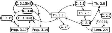
Figure 1: Road map of the main results and assumptions.

We complement our stability results in Section 4 with a discussion on how one can use existing results in the literature to obtain convergence of $(\theta_{i})_{i\geq 0}$ to a zero of $h$. Finally, we apply our theory to a new stochastic approximation expectation maximisation algorithm involving particle independent Metropolis–Hastings sampling in Section 5.

2 General stability results

We denote throughout the article the probability distribution associated to the process $(\theta_{i},X_{i})_{i\geq 0}$ defined in Algorithm 1.1 and starting at $(\theta_{0},X_{0})\equiv(\theta,x)\in\Theta\times\mathsf{X}$ as $\mathbb{P}_{\theta,x}(\cdot)$ and the associated expectation as $\mathbb{E}_{\theta,x}[\cdot]$. For any subset $A\subset E$ of some space $E$, we denote $A^{c}$ its complement in $E$. We also denote $\langle\cdot,\cdot\rangle$ the standard inner product and $|\cdot|$ the associated norm on $\Theta\subset\mathbb{R}^{d}$. We also use the notation $a\vee b:=\max\{a,b\}$ and $a\wedge b:=\min\{a,b\}$.

The approach we develop relies on the existence of a Lyapunov function $w\mathchoice{\nobreak\,\colon}{\nobreak\,\colon}{\nobreak\,\colon\;}{\nobreak\,\colon\;}\Theta\rightarrow[0,\infty)$ for the recursion on $\theta$ and the subsequent proof that $\{w(\theta_{i})\}$ is $\mathbb{P}_{\theta,x}$-a.s. under some adequate level. For any $M>0$, we define the level sets $\mathcal{W}_{M}:=\{\theta\in\Theta\colon\ w(\theta)\leq M\}$. Our general stability results are inspired by a proof due to Benveniste, Metivier and Priouret [8], Theorem 17, page 239, but differ in many respects as we shall see.

We consider two different settings concerning the way $w$ behaves on the boundary $\partial\Theta$ of $\Theta$. Section 2.1 assumes that $\lim_{\theta\rightarrow\partial\Theta}w(\theta)=\infty$, which is well suited for example to the case $\Theta=\mathbb{R}$ and $\partial\Theta=\{-\infty,\infty\}$. Section 2.2 considers the case where $w$ may not be unbounded, which requires stronger assumptions on the behaviour of $w$. This setting subsumes for example the case where $\Theta\subset\mathbb{R}$ and $\partial\Theta$ contains some points on the real line. Both of the scenarios share the following set of assumptions.

Condition 2.1.

There exists a twice continuously differentiable function $w\mathchoice{\nobreak\,\colon}{\nobreak\,\colon}{\nobreak\,\colon\;}{\nobreak\,\colon\;}\Theta\rightarrow[0,\infty)$ such that

1. [(iii)]

2. the Hessian matrix $\operatorname{Hess}_{w}\mathchoice{\nobreak\,\colon}{\nobreak\,\colon}{\nobreak\,\colon\;}{\nobreak\,\colon\;}\Theta\to\mathbb{R}^{d\times d}$ of $w$ is bounded so that

   $$C_{w}:=\sup_{\theta\in\Theta}\sup_{|\theta_{0}|=1}\bigl{|}\operatorname{Hess}_{w}(\theta)\theta_{0}\bigr{|}<\infty,$$

3. the projection sets are increasing subsets of $\Theta$, that is, $\mathcal{R}_{i}\subset\mathcal{R}_{i+1}$ for all $i\geq 0$, and $\hat{\Theta}:=\bigcup_{i=0}^{\infty}\mathcal{R}_{i}\subset\Theta$,

4. there exists a constant $M_{0}>0$ such that for any $\theta\in\mathcal{W}_{M_{0}}^{c}\cap\hat{\Theta}$

   $$\bigl{\langle}\nabla w(\theta),h(\theta)\bigr{\rangle}\leq 0,$$

5. the family of random variables $\{\theta_{i}^{\mathrm{proj}}\}_{i\geq 1}$ satisfies for all $i\geq 1$ whenever $\theta_{i}^{\ast}\notin\mathcal{R}_{i}$

   $$\theta_{i}^{\mathrm{proj}}\in\mathcal{R}_{i}\quad\mbox{and}\quad w\bigl{(}\theta_{i}^{\mathrm{proj}}\bigr{)}\leq w\bigl{(}\theta^{\ast}_{i}\bigr{)}\qquad\mathbb{P}_{\theta,x}\mbox{-a.s.},$$

6. there exists constants $\alpha_{w},c\in[0,\infty)$ and a non-decreasing sequence of constants $\xi_{i}\in[1,\infty)$ satisfying $\sup_{\theta\in\mathcal{R}_{i}}|\nabla w(\theta)|\leq c\xi_{i}^{\alpha_{w}}$ for all $i\geq 0$.

Remark 2.2.

Condition 2.1

1. [(iii)]

2. Can often be established by introducing a Lyapunov function defined through $w:=\psi\circ\tilde{w}$, where $\psi\mathchoice{\nobreak\,\colon}{\nobreak\,\colon}{\nobreak\,\colon\;}{\nobreak\,\colon\;}[0,\infty)\to[0,\infty)$ is a suitable concave function modifying the values of another Lyapunov function $\tilde{w}$ which satisfies the drift condition (iii) but does not have finite second derivatives; see [8], Remark on page 239.

3. Is often satisfied with $\hat{\Theta}=\Theta$, but accomodates also projections sets which do not cover $\Theta$, but only certain admissible values $\hat{\Theta}\subsetneq\Theta$. As an extreme case, this allows to use the present framework to check that a fixed projection does not induce spurious attractors on the boundary of $\hat{\Theta}$. Notice also that the function $H(\theta,x)$ and the corresponding mean field $h(\theta)$ need only be defined for values $\theta\in\hat{\Theta}$.

4. Will be replaced with a stricter drift in Theorem 2.8, where $w$ is not required to diverge on the boundary $\partial\hat{\Theta}$.

5. Is satisfied trivially by the choices $\theta_{i}^{\mathrm{proj}}:=\theta_{i-1}$ and $\theta_{i}^{\mathrm{proj}}:=\Pi_{\mathcal{R}_{i}}(\theta_{i}^{*})$, if the projection sets are defined as the level sets of the Lyapunov function, that is $\mathcal{R}_{i}:=\mathcal{W}_{M_{i}}$ for some $M_{i}>0$. In the Markovian case, the projections are assumed to satisfy an additional continuity condition; see Theorem 3.3.

6. Involves in practice a sequence that grows at most at a rate $\xi_{i}:=i\vee 1$, with some power $\alpha_{w}\in[0,1)$. The sequence $\xi_{i}$ plays a central role also in controlling the ergodicity rate of the Markov chain in $\mathcal{R}_{i}$; see Remark 3.2.

Hereafter, we denote the ‘centred’ version of $H$ as $\bar{H}(\theta,x):=H(\theta,x)-h(\theta)$. For the stability results, we shall introduce the following general condition on the noise sequence. In general terms, it is related to the rate at which $\{\theta_{i}\}$ may approach $\partial\hat{\Theta}$ in relation to the growth of $|H(\theta,x)|$ and the loss of ergodicity of $\{P_{\theta}\}$. Establishing practical and realistic conditions under which this assumption holds will be the topic of Section 3.

Condition 2.3.

For any $(\theta,x)\in\mathcal{R}_{0}\times\mathsf{X}$ it holds that

1. [(iii)]

2. $\mathbb{P}_{\theta,x}\Bigl{(}\displaystyle\lim_{i\to\infty}\Gamma_{i+1}\bigl{|}\nabla w(\theta_{i})\bigr{|}\cdot\bigl{|}H(\theta_{i},X_{i+1})\bigr{|}=0\Bigr{)}=1$,

3. $\mathbb{E}_{\theta,x}\Biggl{[}{\displaystyle\sum_{i=0}^{\infty}}\Gamma_{i+1}^{2}\bigl{|}H(\theta_{i},X_{i+1})\bigr{|}^{2}\Biggr{]}<\infty$,

4. $\mathbb{E}_{\theta,x}\Biggl{[}\displaystyle\sup_{k\geq 0}\Biggl{|}\sum_{i=0}^{k}\Gamma_{i+1}\bigl{\langle}\nabla w(\theta_{i}),\bar{H}(\theta_{i},X_{i+1})\bigr{\rangle}\Biggr{|}\Biggr{]}<\infty$.

In what follows, we shall focus on a single condition implying Condition 2.3(i) and (ii). It is slightly more stringent, but more convenient to check in practice.

Lemma 2.4

Suppose Condition 2.1 holds and

$$\mathbb{E}_{\theta,x}\Biggl{[}{\sum_{i=0}^{\infty}}\Gamma_{i+1}^{2}\xi_{i}^{2\alpha_{w}}\bigl{|}H(\theta_{i},X_{i+1})\bigr{|}^{2}\Biggr{]}<\infty.$$ (2)

Then, Condition 2.3(i) and (ii) hold.

Proof.

Note first that Condition 2.3(ii) holds trivially, because $\xi_{i}^{2\alpha_{w}}\geq 1$. For Condition 2.3(i), consider

$$\mathbb{E}_{\theta,x}\Biggl{[}{\sum_{i=0}^{\infty}}\bigl{(}\Gamma_{i+1}\bigl{|}\nabla w(\theta_{i})\bigr{|}\cdot\bigl{|}H(\theta_{i},X_{i+1})\bigr{|}\bigr{)}^{2}\Biggr{]}\leq c^{2}\mathbb{E}_{\theta,x}\Biggl{[}{\sum_{i=0}^{\infty}}\Gamma_{i+1}^{2}\xi_{i}^{2\alpha_{w}}\bigl{|}H(\theta_{i},X_{i+1})\bigr{|}^{2}\Biggr{]}.$$

∎

2.1 Unbounded Lyapunov function

When $\lim_{\theta\to\partial\hat{\Theta}}w(\theta)=\infty$, it is enough to show that the sequence $w(\theta_{i})$ is bounded in order to ensure the stability of $\theta_{i}$.

Theorem 2.5

Assume Conditions 2.1 and 2.3 hold. Then, for any $(\theta,x)\in\mathcal{R}_{0}\times\mathsf{X}$

$$\mathbb{P}_{\theta,x}\Bigl{(}\limsup_{i\to\infty}w(\theta_{i})<\infty\Bigr{)}=1.$$

Proof.

To show the $\mathbb{P}_{\theta,x}$-a.s. boundedness of $\{w(\theta_{i})\}$ we fix $(\theta,x)\in\mathcal{R}_{0}\times\mathsf{X}$ and introduce the following quantities. Let $M_{0}<M_{1}<\cdots<M_{n}\to\infty$ be an increasing sequence tending to infinity and consider the level sets $\mathcal{W}_{M_{i}}\subset\Theta$. We assume that $M_{0}$ is chosen large enough so that $\theta_{0}=\theta\in\mathcal{W}_{M_{0}}$. For any $n\geq 0$, we define the first exit time of $\theta_{i}$ from the level set $\mathcal{W}_{M_{n}}$ as

$$\sigma_{n}:=\inf\{i\geq 0\colon\ \theta_{i}\notin\mathcal{W}_{M_{n}}\},$$

with the usual convention that $\inf\{\varnothing\}=\infty$. For any $n\geq 0$, we define the time following the last exit of $\theta_{i}$ from $\mathcal{W}_{M_{0}}$ before $\sigma_{n}$ as

$$\tau_{n}:=1+\sup\{i\leq\sigma_{n}\colon\ \theta_{i}\in\mathcal{W}_{M_{0}}\},$$

which is finite at least whenever $\sigma_{n}$ is finite by our assumption that $\theta_{0}\in\mathcal{W}_{M_{0}}$. With these definitions, the claim holds once we show that $\lim_{n\to\infty}\mathbb{P}_{\theta,x}(\sigma_{n}<\infty)=0$.

To begin with, define for $n\geq 1$ the following sets characterising the jumps out of $\mathcal{W}_{M_{0}}$

$$D_{n}:=\biggl{\{}\mathbb{I}\{\tau_{n}<\infty\}\bigl{[}w(\theta_{\tau_{n}})-w(\theta_{\tau_{n}-1})\bigr{]}\leq\frac{M_{n}-M_{0}}{2}\biggr{\}}.$$

We first show that $\lim_{n\to\infty}\mathbb{P}_{\theta,x}(D_{n})=1$. Clearly

$$\tilde{D}_{n}:=\biggl{\{}\sup_{i\geq 0}\bigl{[}w(\theta_{i+1})-w(\theta_{i})\bigr{]}\leq\frac{M_{n}-M_{0}}{2}\biggr{\}}\subset D_{n}$$ (3)

and since $M_{n}\to\infty$, one has $\{\sup_{i\geq 0}[w(\theta_{i+1})-w(\theta_{i})]<\infty\}=\bigcup_{n=1}^{\infty}\tilde{D}_{n}$. Lemma 2.6 shows that $1=\mathbb{P}_{\theta,x}(\bigcup_{n=1}^{\infty}\tilde{D}_{n})=\lim_{n\rightarrow\infty}\mathbb{P}_{\theta,x}(\tilde{D}_{n})\leq\lim_{n\rightarrow\infty}\mathbb{P}_{\theta,x}(D_{n})$ because $\tilde{D}_{n}$ is an increasing sequence and by (3), respectively.

Now, it remains to focus on proving that

$$\lim_{n\rightarrow\infty}\mathbb{P}_{\theta,x}\bigl{(}D_{n}\cap\{\sigma_{n}<\infty\}\bigr{)}=0.$$

In order to achieve this observe first that $w(\theta_{\sigma_{n}})-w(\theta_{\tau_{n}-1})\geq M_{n}-M_{0}$ on $\{\sigma_{n}<\infty\},$ implying that on $D_{n}\cap\{\sigma_{n}<\infty\}$,

$$w(\theta_{\sigma_{n}})-w(\theta_{\tau_{n}})=w(\theta_{\sigma_{n}})-w(\theta_{\tau_{n}-1})-\bigl{[}w(\theta_{\tau_{n}})-w(\theta_{\tau_{n}-1})\bigr{]}\geq\frac{M_{n}-M_{0}}{2}.$$

This allows us to deduce the following bound

$$\mathbb{P}_{\theta,x}\bigl{(}D_{n}\cap\{\sigma_{n}<\infty\}\bigr{)} = \mathbb{E}_{\theta,x}\bigl{[}\mathbb{I}\bigl{\{}D_{n}\cap\{\sigma_{n}<\infty\}\bigr{\}}\bigr{]}$$

$$\leq \mathbb{E}_{\theta,x}\biggl{[}\mathbb{I}\bigl{\{}D_{n}\cap\{\sigma_{n}<\infty\}\bigr{\}}\frac{w(\theta_{\sigma_{n}})-w(\theta_{\tau_{n}})}{({1}/{2})(M_{n}-M_{0})}\biggr{]}$$

$$\leq \frac{2}{M_{n}-M_{0}}\mathbb{E}_{\theta,x}\bigl{[}\mathbb{I}\{\sigma_{n}<\infty\}\bigl{[}w(\theta_{\sigma_{n}})-w(\theta_{\tau_{n}})\bigr{]}\bigr{]}.$$

Since $M_{n}\to\infty$, the proof will be finished once we show that

$$\sup_{n\geq 0}\mathbb{E}_{\theta,x}\bigl{[}\mathbb{I}\{\sigma_{n}<\infty\}\bigl{[}w(\theta_{\sigma_{n}})-w(\theta_{\tau_{n}})\bigr{]}\bigr{]}<\infty.$$ (4)

Thanks to Condition 2.1(iv), we have for any $i\geq 0$ that $w(\theta_{i+1})\leq w(\theta_{i+1}^{*})$ and consequently

$$w(\theta_{i+1})-w(\theta_{i}) \leq \Gamma_{i+1}\bigl{\langle}\nabla w(\theta_{i}),h(\theta_{i})\bigr{\rangle}$$

$${}+\Gamma_{i+1}\bigl{\langle}\nabla w(\theta_{i}),\bar{H}(\theta_{i},X_{i+1})\bigr{\rangle}+\Gamma_{i+1}^{2}\frac{C_{w}}{2}\bigl{|}H(\theta_{i},X_{i+1})\bigr{|}^{2}.$$

So in particular, since $\langle\nabla w(\theta_{i}),h(\theta_{i})\rangle\leq 0$ whenever $\theta_{i}\in\mathcal{W}_{M_{0}}^{c}$,

$$\mathbb{I}\{\sigma_{n}<\infty\}\bigl{[}w(\theta_{\sigma_{n}})-w(\theta_{\tau_{n}})\bigr{]}$$

$$\quad=\mathbb{I}\{\sigma_{n}<\infty\}{\sum_{i=\tau_{n}}^{\sigma_{n}-1}}\bigl{[}w(\theta_{i+1})-w(\theta_{i})\bigr{]}$$

$$\quad\leq\mathbb{I}\{\sigma_{n}<\infty\}\Biggl{(}{\sum_{i=\tau_{n}}^{\sigma_{n}-1}}\Gamma_{i+1}\bigl{\langle}\nabla w(\theta_{i}),\bar{H}(\theta_{i},X_{i+1})\bigr{\rangle}+\Gamma_{i+1}^{2}\frac{C_{w}}{2}\bigl{|}H(\theta_{i},X_{i+1})\bigr{|}^{2}\Biggr{)}.$$

Recall the following estimate for partial sums

$$\Biggl{|}\sum_{i=j}^{k}a_{i}\Biggr{|}=\Biggl{|}\sum_{i=0}^{k}a_{i}-\sum_{i=0}^{j-1}a_{i}\Biggr{|}\leq\Biggl{|}\sum_{i=0}^{k}a_{i}\Biggr{|}+\Biggl{|}\sum_{i=0}^{j-1}a_{i}\Biggr{|}\leq 2\sup_{k\geq 0}\Biggl{|}\sum_{i=0}^{k}a_{i}\Biggr{|},$$ (5)

implying in our case that

$$\frac{1}{2}\mathbb{I}\{\sigma_{n}<\infty\}\bigl{[}w(\theta_{\sigma_{n}})-w(\theta_{\tau_{n}})\bigr{]}$$

$$\quad\leq\mathbb{I}\{\sigma_{n}<\infty\}\Biggl{(}\sup_{k\geq 0}\Biggl{|}\sum_{i=0}^{k}\Gamma_{i+1}\bigl{\langle}\nabla w(\theta_{i}),\bar{H}(\theta_{i},X_{i+1})\bigr{\rangle}\Biggr{|}+\sum_{i=0}^{\infty}\Gamma_{i+1}^{2}\frac{C_{w}}{2}\bigl{|}H(\theta_{i},X_{i+1})\bigr{|}^{2}\Biggr{)}.$$

Now, Condition 2.3(ii) and (iii) imply (4) allowing us to conclude. ∎

Lemma 2.6

Under Condition 2.3 we have, $\mathbb{P}_{\theta,x}$-almost surely

$$\limsup_{i\to\infty}\bigl{[}w(\theta_{i+1})-w(\theta_{i})\bigr{]} \leq 0,$$ (6)

$$\sup_{i\geq 0}\bigl{[}w(\theta_{i+1})-w(\theta_{i})\bigr{]} < \infty.$$ (7)

Proof.

We first prove that $\lim_{i\rightarrow\infty}|w(\theta_{i+1}^{\ast})-w(\theta_{i})|=0$, $\mathbb{P}_{\theta,x}$-a.s. By a Taylor expansion, we get

$$\bigl{|}w\bigl{(}\theta_{i+1}^{\ast}\bigr{)}-w(\theta_{i})\bigr{|}\leq\bigl{|}\nabla w(\theta_{i})\bigr{|}\cdot\bigl{|}\Gamma_{i+1}H(\theta_{i},X_{i+1})\bigr{|}+\Gamma_{i+1}^{2}C_{w}\bigl{|}H(\theta_{i},X_{i+1})\bigr{|}^{2}.$$

The terms on the right converge to zero $\mathbb{P}_{\theta,x}$-a.s. by Condition 2.3(i) and (ii), respectively. Now, (6) follows since by Condition 2.1(iv) $w(\theta_{i+1})-w(\theta_{i})\leq w(\theta_{i+1}^{*})-w(\theta_{i})$. We conclude by noting that (7) follows directly from (6). ∎

2.2 Bounded Lyapunov function

In the previous section, the Lyapunov function satisfied $\lim_{\theta\to\partial\hat{\Theta}}w(\theta)=\infty$. If this is not the case, we need to replace Condition 2.1(iii) with a more stringent condition quantifying the drift outside $\mathcal{W}_{M_{0}}$, while not requiring $\lim_{\theta\to\partial\hat{\Theta}}w(\theta)=\infty$.

Condition 2.7.

The Lyapunov function and the step size sequence satisfy

$$\delta_{i}:=\inf_{\theta\in\mathcal{R}_{i}\setminus\mathcal{W}_{M_{0}}}-\bigl{\langle}\nabla w(\theta),h(\theta)\bigr{\rangle}>0\quad\mbox{and}\quad\sum_{i=1}^{\infty}\Gamma_{i}\delta_{i}=\infty\qquad\mathbb{P}_{\theta,x}\mbox{-almost surely}.$$

Theorem 2.8

Assume Conditions 2.1, 2.3 and 2.7 hold, and in addition that the following condition on the noise holds

$$\lim_{m\to\infty}\sup_{k>m}\Biggl{|}\sum_{i=m}^{k}\Gamma_{i+1}\bigl{\langle}\nabla w(\theta_{i}),\bar{H}(\theta_{i},X_{i+1})\bigr{\rangle}\Biggr{|}=0.$$ (8)

Then for any $M>M_{0}$, the tails of the trajectories of $\{\theta_{i}\}$ are eventually contained within $\mathcal{W}_{M}$ $\mathbb{P}_{\theta,x}$-a.s., that is,

$$\mathbb{P}_{\theta,x}\biggl{(}\bigcup_{m\geq 0}\bigcap_{n\geq m}\{\theta_{n}\in\mathcal{W}_{M}\}\biggr{)}=1.$$

Proof.

We first show that $\theta_{n}$ must visit $\mathcal{W}_{M_{0}}$ infinitely often $\mathbb{P}_{\theta,x}$-a.s., in other words

$$\mathbb{P}_{\theta,x}\biggl{(}{\bigcup_{m\geq 1}}{\bigcap_{n\geq m}}\{\theta_{n}\notin\mathcal{W}_{M_{0}}\}\biggr{)}=0.$$ (9)

For any $m\geq 0$, we define the hitting times $\kappa_{m}:=\inf\{i>m\colon\ \theta_{i}\in\mathcal{W}_{M_{0}}\}$ and notice that

$${\bigcup_{m\geq 1}}{\bigcap_{n\geq m}}\{\theta_{n}\notin\mathcal{W}_{M_{0}}\}={\bigcup_{m\geq 1}}\{\theta_{m}\notin\mathcal{W}_{M_{0}}\}\cap\{\kappa_{m}=\infty\}.$$

Recall that for any $i\geq 0$

$$w(\theta_{i+1})-w(\theta_{i}) \leq \Gamma_{i+1}\bigl{\langle}\nabla w(\theta_{i}),h(\theta_{i})\bigr{\rangle}$$

$${}+\Gamma_{i+1}\bigl{\langle}\nabla w(\theta_{i}),\bar{H}(\theta_{i},X_{i+1})\bigr{\rangle}+\Gamma_{i+1}^{2}\frac{C_{w}}{2}\bigl{|}H(\theta_{i},X_{i+1})\bigr{|}^{2}.$$

So in particular, and thanks to Condition 2.7, for $n>m$

$$\mathbb{I}\{\theta_{m}\notin\mathcal{W}_{M_{0}}\}\bigl{[}w(\theta_{n\wedge\kappa_{m}})-w(\theta_{m})\bigr{]}$$

$$\quad=\mathbb{I}\{\theta_{m}\notin\mathcal{W}_{M_{0}}\}{\sum_{i=m}^{(n\wedge\kappa_{m})-1}}\mathbb{I}\{\theta_{i}\notin\mathcal{W}_{M_{0}}\}\bigl{[}w(\theta_{i+1})-w(\theta_{i})\bigr{]}$$

$$\quad\leq\mathbb{I}\{\theta_{m}\notin\mathcal{W}_{M_{0}}\}{\sum_{i=m}^{(n\wedge\kappa_{m})-1}}\Gamma_{i+1}\biggl{[}-\delta_{i}+\bigl{\langle}\nabla w(\theta_{i}),\bar{H}(\theta_{i},X_{i+1})\bigr{\rangle}+\Gamma_{i+1}\frac{C_{w}}{2}\bigl{|}H(\theta_{i},X_{i+1})\bigr{|}^{2}\biggr{]}.$$

From this, we obtain the following inequality holding $\mathbb{P}_{\theta,x}$-a.s. on $\{\theta_{m}\notin\mathcal{W}_{M_{0}}\}$ for any $n>m$

$$\mathbb{E}_{\theta,x}\Biggl{[}\mathbb{I}\{\kappa_{m}=\infty\}{\sum_{i=m}^{n-1}}\Gamma_{i+1}\delta_{i}\Bigl{|}\mathcal{F}_{m}\Biggr{]}-w(\theta_{m})$$

$$\quad\leq\mathbb{E}_{\theta,x}\Biggl{[}\mathbb{I}\{\kappa_{m}=\infty\}{\sum_{i=m}^{n-1}}\Gamma_{i+1}\bigl{\langle}\nabla w(\theta_{i}),\bar{H}(\theta_{i},X_{i+1})\bigr{\rangle}$$ (10)

$$\quad\hphantom{\leq\mathbb{E}_{\theta,x}\Biggl{[}\mathbb{I}\{\kappa_{m}=\infty\}{\sum_{i=m}^{n-1}}}{}+\Gamma_{i+1}^{2}\frac{C_{w}}{2}\bigl{|}H(\theta_{i},X_{i+1})\bigr{|}^{2}\Bigl{|}\mathcal{F}_{m}\Biggr{]}.$$

Using this inequality, we shall see that for any $m>0$

$$\mathbb{P}_{\theta,x}\bigl{(}\{\theta_{m}\notin\mathcal{W}_{M_{0}}\}\cap\{\kappa_{m}=\infty\}\bigr{)}=0.$$ (11)

Suppose the contrary, $\mathbb{P}_{\theta,x}(\{\theta_{m}\notin\mathcal{W}_{M_{0}}\}\cap\{\kappa_{m}=\infty\})>0$. Then, because of Condition 2.7, we observe that the conditional expectation on the left hand side of (2.2) necessarily tends to infinity almost surely as $n\to\infty$. Denote then the conditional expectation on the right hand side of (2.2) by $E_{\theta,x}^{(m,n)}$. As in the proof of Theorem 2.5, we have the following upper bound

$$\mathbb{E}_{\theta,x}\bigl{[}E_{\theta,x}^{(m,n)}\bigr{]}\leq\mathbb{E}_{\theta,x}\Biggl{[}\sup_{k\geq 0}\Biggl{|}\sum_{i=0}^{k}\Gamma_{i+1}\bigl{\langle}\nabla w(\theta_{i}),\bar{H}(\theta_{i},X_{i+1})\bigr{\rangle}\Biggr{|}+\sum_{i=0}^{\infty}\Gamma_{i+1}^{2}\frac{C_{w}}{2}\bigl{|}H(\theta_{i},X_{i+1})\bigr{|}^{2}\Biggr{]},$$

which is finite by Condition 2.3 and independent of $m$ and $n$. By letting $n\to\infty$ we end up with a contradiction, unless (11) holds. Consequently, the event

$${\bigcup_{m\geq 1}}\{\theta_{m}\notin\mathcal{W}_{M_{0}}\}\cap\{\kappa_{m}=\infty\}$$

has null probability and we obtain (9).

We now show that for any fixed $M>M_{0}$

$$\mathbb{P}_{\theta,x}\biggl{(}\bigcup_{m\geq 0}\bigcap_{n\geq m}\{\theta_{n}\in\mathcal{W}_{M}\}\biggr{)}=1.$$

We are going to apply Lemma 2.9 below with $\delta=M-M_{0}>0$ to the events

$$A_{m}=\{\theta_{m}\in\mathcal{W}_{M_{0}}\}\cap{\bigcup_{k>m}}\{\theta_{k}\notin\mathcal{W}_{M}\},$$

and denote

$$B_{m}:=\{\theta_{m}\in\mathcal{W}_{M_{0}}\}\setminus A_{m}=\{\theta_{m}\in\mathcal{W}_{M_{0}}\}\cap{\bigcap_{k>m}}\{\theta_{k}\in\mathcal{W}_{M}\}.$$

We may write

$${\bigcap_{n\geq 1}}{\bigcup_{m\geq n}}\{\theta_{m}\in\mathcal{W}_{M_{0}}\} = {\bigcap_{n\geq 1}}{\bigcup_{m\geq n}}A_{m}\cup B_{m}$$

$$= {\bigcap_{n\geq 1}}\biggl{[}\biggl{(}{\bigcup_{m\geq n}}A_{m}\biggr{)}\cup\biggl{(}{\bigcup_{m\geq n}}B_{m}\biggr{)}\biggr{]}.$$

Now, since ${\bigcup_{m\geq n}}A_{m}$ and ${\bigcup_{m\geq n}}B_{m}$ are both decreasing events with respect to $n\to\infty$, we have

$$1 = \lim_{n\rightarrow\infty}\mathbb{P}_{\theta,x}\biggl{(}{\bigcup_{m\geq n}}\{\theta_{m}\in\mathcal{W}_{M_{0}}\}\biggr{)}$$

$$= \lim_{n\rightarrow\infty}\biggl{[}\mathbb{P}_{\theta,x}\biggl{(}{\bigcup_{m\geq n}}A_{m}\biggr{)}+\mathbb{P}_{\theta,x}\biggl{(}{\bigcup_{m\geq n}}B_{m}\biggr{)}-\mathbb{P}_{\theta,x}\biggl{(}{\bigcup_{m\geq n}}A_{m}\cap{\bigcup_{m\geq n}}B_{m}\biggr{)}\biggr{]}.$$

By Lemma 2.9, $\lim_{n\to\infty}\mathbb{P}_{\theta,x}(\bigcup_{m\geq n}A_{m})=0$, so we end up with $\lim_{n\rightarrow\infty}\mathbb{P}_{\theta,x}(\bigcup_{m\geq n}B_{m})=1$, implying the claim. ∎

Lemma 2.9

Assume the conditions of Theorem 2.8, let $\delta>0$ and denote

$$A_{m}:=\{\theta_{m}\in\mathcal{W}_{M_{0}}\}\cap{\bigcup_{k>m}}\{\theta_{k}\notin\mathcal{W}_{M_{0}+\delta}\}.$$

Then, $\lim_{n\to\infty}\mathbb{P}_{\theta,x}(\bigcup_{m\geq n}A_{m})=0$.

Proof.

Define the random times $\sigma_{m}:=\inf\{i>m\colon\ \theta_{i}\notin\mathcal{W}_{M_{0}+\delta}\}$ and $\tau_{m}:=\sup\{i\in[m,\sigma_{m})\colon\ \theta_{i}\in\mathcal{W}_{M_{0}}\}+1$, both finite on $A_{m}$. Recall that on $\{\theta_{i}\in\mathcal{W}_{M_{0}}^{c}\}$ we have

$$w(\theta_{i+1})-w(\theta_{i})\leq\Gamma_{i+1}\bigl{\langle}\nabla w(\theta_{i}),\bar{H}(\theta_{i},X_{i+1})\bigr{\rangle}+\Gamma_{i+1}^{2}\frac{C_{w}}{2}\bigl{|}H(\theta_{i},X_{i+1})\bigr{|}^{2},$$

so on $A_{m}$ we may bound

$$w(\theta_{\sigma_{m}})-w(\theta_{\tau_{m}}) \leq \sum_{i=\tau_{m}}^{\sigma_{m}-1}\Gamma_{i+1}\bigl{\langle}\nabla w(\theta_{i}),\bar{H}(\theta_{i},X_{i+1})\bigr{\rangle}+\Gamma_{i+1}^{2}\frac{C_{w}}{2}\bigl{|}H(\theta_{i},X_{i+1})\bigr{|}^{2}$$

$$\leq 2\sup_{k>m}\Biggl{|}\sum_{i=m}^{k}\Gamma_{i+1}\bigl{\langle}\nabla w(\theta_{i}),\bar{H}(\theta_{i},X_{i+1})\bigr{\rangle}\Biggr{|}+\sum_{i=m}^{\infty}\Gamma_{i+1}^{2}\frac{C_{w}}{2}\bigl{|}H(\theta_{i},X_{i+1})\bigr{|}^{2}$$

$$\hphantom{:}=: C_{m}$$

by a similar argument as in (5). On $A_{m}$ one clearly has $w(\theta_{\sigma_{m}})-w(\theta_{\tau_{m}-1})>\delta$, implying that $C_{m}+w(\theta_{\tau_{m}})-w(\theta_{\tau_{m}-1})>\delta$. We deduce that

$$\tilde{A}_{m}:=\Bigl{\{}C_{m}+\sup_{i\geq m}\bigl{[}w(\theta_{i+1})-w(\theta_{i})\bigr{]}>\delta\Bigr{\}}\supset A_{m}.$$

The sets $\tilde{A}_{m}$ are clearly decreasing with respect to $m$ and $\lim_{m\to\infty}\mathbb{P}_{\theta,x}(\tilde{A}_{m})=0$ by Lemma 2.6 and because Condition 2.3(ii) and (8) imply $\lim_{m\to\infty}C_{m}=0$. This concludes the proof, because $\bigcup_{m\geq n}A_{m}\subset\bigcup_{m\geq n}\tilde{A}_{m}=\tilde{A}_{n}$. ∎

3 Verifying noise conditions

The aim of this section is to provide verifiable conditions which will imply the conditions of the stability theorems in Section 2. We proceed progressively and start by a general result in Theorem 3.3 which ensures both Condition 2.3 and that in (8) hold given a set of abstract conditions involving some expectations as well as properties of the solutions of the Poisson equation.

Condition 3.1, required in Theorem 3.3, shall be verified in detail below for a family of geometrically ergodic Markov kernels. In Section 3.1, we first gather general known results related to Condition 3.1(ii) and (iii). In Section 3.2, we consider the case where the mapping $\theta\to P_{\theta}$ is Hölder continuous, which allows us to establish Condition 3.1(iv). In Section 3.3, we consider the case where the aforementioned Hölder continuity may not hold, and a continuity is enforced by using a random step size sequence, allowing us to recover Condition 3.1(iv) in such situations.

Condition 3.1.

Condition 2.1 holds with constants $(\xi_{i})_{i\geq 0}$ and $\alpha_{w}\in(0,\infty)$. For all $\theta\in\hat{\Theta}$, the solution $g_{\theta}\mathchoice{\nobreak\,\colon}{\nobreak\,\colon}{\nobreak\,\colon\;}{\nobreak\,\colon\;}\mathsf{X}\to\Theta$ to the Poisson equation $g_{\theta}(x)-P_{\theta}g_{\theta}(x)\equiv\bar{H}(\theta,x)$ exists and for all $i\geq 0$ the step size $\Gamma_{i+1}$ is independent of $\mathcal{F}_{i}$ and $X_{i+1}$. Moreover, there exist a measurable function $V\mathchoice{\nobreak\,\colon}{\nobreak\,\colon}{\nobreak\,\colon\;}{\nobreak\,\colon\;}\mathsf{X}\to[1,\infty)$ and constants $c<\infty$, $\beta_{H},\beta_{g}\in[0,1/2]$ and $\alpha_{g},\alpha_{H},\alpha_{V}\in[0,\infty)$ such that for all $(\theta,x)\in\mathcal{R}_{0}\times\mathsf{X}$

1. [(vii)]

2. $\displaystyle\sup_{\theta\in\mathcal{R}_{i}}\bigl{|}H(\theta,x)\bigr{|}\leq c\xi_{i}^{\alpha_{H}}V^{\beta_{H}}(x)$,

3. $\mathbb{E}_{\theta,x}\bigl{[}V(X_{i})\bigr{]}\leq c\xi_{i}^{\alpha_{V}}V(x)$,

4. $\displaystyle\sup_{\theta\in\mathcal{R}_{i}}\bigl{[}\bigl{|}g_{\theta}(x)\bigr{|}+\bigl{|}P_{\theta}g_{\theta}(x)\bigr{|}\bigr{]}\leq c\xi_{i}^{\alpha_{g}}V^{\beta_{g}}(x)$,

5. $\displaystyle\sum_{i=1}^{\infty}\mathbb{E}[\Gamma_{i+1}]\xi_{i}^{\alpha_{w}}\mathbb{E}_{\theta,x}\bigl{[}\bigl{|}P_{\theta_{i}}g_{\theta_{i}}(X_{i})-P_{\theta_{i-1}}g_{\theta_{i-1}}(X_{i})\bigr{|}\bigr{]}<\infty$,

6. $\displaystyle\sum_{i=1}^{\infty}\mathbb{E}\bigl{[}\Gamma_{i}^{2}\bigr{]}\xi_{i}^{2\alpha_{w}+2((\alpha_{H}+\beta_{H}\alpha_{V})\vee(\alpha_{g}+\beta_{g}\alpha_{V}))}<\infty$,

7. $\displaystyle\sum_{i=1}^{\infty}\mathbb{E}[\Gamma_{i+1}\Gamma_{i}]\xi_{i}^{\alpha_{H}+\alpha_{g}+(\beta_{H}+\beta_{g})\alpha_{V}}<\infty$,

8. $\displaystyle\sum_{i=1}^{\infty}\bigl{|}\mathbb{E}[\Gamma_{i+1}-\Gamma_{i}]\bigr{|}\xi_{i}^{\alpha_{w}+\alpha_{g}+\beta_{g}\alpha_{V}}<\infty$,

where we write $\mathbb{E}:=\mathbb{E}_{\theta,x}$ whenever the expectation does not depend on $\theta$ and $x$.

Remark 3.2.

These assumptions call for various comments of practical relevance to the actual implementation of the algorithm with expanding projections. Once $H(\cdot,\cdot)$ and $\{P_{\theta}\}_{\theta\in\Theta}$ are chosen the user is left with the choice of $(\xi_{i})_{i\geq 0}$ and $(\Gamma_{i})_{i\geq 0}$, which must in particular satisfy the summability conditions above. For the purpose of efficiency we would like $(\xi_{i})_{i\geq 0}$ to grow as fast as possible, as we may otherwise slow convergence down. A common choice for the step-size sequence is $\Gamma_{i}=ci^{-\eta}$ for some constants $c\in(0,\infty)$ and $\eta\in(1/2,1]$ – this implies a required condition to establish convergence. The sequence $(\xi_{i})_{i\geq 0}$ is determined by the user through the choice of the sequence of reprojection sets $(\mathcal{R}_{i})_{i\geq 0}$ and we point out that the constants $\alpha_{H},\alpha_{V}$ and $\alpha_{g}$ typically depend on that choice (whereas $\beta_{H}$ and $\beta_{g}$ typically do not). We show how these constants can be obtained from the properties of $\{P_{\theta}\}_{\theta\in\Theta}$ in Sections 3.1–3.3. Now if $(\xi_{i})_{i\geq 0}$ is increasing at a rate slower than any power sequence, for example of the order $\log i$ or $i^{(\log i)^{-p}}$ for some $p\in(0,1)$, then it is easy to see that the summability conditions (v)–(vii) are always satisfied. In the situation where $\xi_{i}=i^{p}$ for $p\in(0,1]$, then the conditions (v)–(vii) require stricter assumptions on $\eta$ and the constants $\alpha_{H},\alpha_{V},\alpha_{g},\beta_{H}$ and $\beta_{g}$ which may not be satisfiable. We however point out a possible sub-optimality of the results stated above. Indeed, in order to simplify presentation we have decided to quantify the growth of the various quantities involved in the algorithm in terms of powers of $(\xi_{i})_{i\geq 0}$ only, whereas other scales may be possible, such as $\log(\xi_{i})$, in which case some of the constants $\alpha_{H},\alpha_{V}$ or $\alpha_{g}$ may be taken arbitrarily small in the statement above. It is also possible to revisit our proofs with such more precise estimates and obtain a set of weaker assumptions.

In practice, the conditions (iii) and (iv) add more requirements which are inter-related with (v)–(vii); Propositions 3.17 and 3.19 summarise the conditions when $\theta\mapsto P_{\theta}$ admits a Hölder-continuity, and when a random step size sequence is used to satisfy (iv), respectively. Appendix D contains a summary of the related constants.

Theorem 3.3

Suppose Conditions 2.1 and 3.1 hold and for all $i\geq 0$ the projections satisfy $|\theta_{i+1}-\theta_{i}|\leq|\theta_{i+1}^{*}-\theta_{i}|$. Then, for all $(\theta,x)\in\mathcal{R}_{0}\times\mathsf{X}$,

$$\mathbb{E}_{\theta,x}\Biggl{[}{\sum_{i=0}^{\infty}}\Gamma_{i+1}^{2}\xi_{i}^{2\alpha_{w}}\bigl{|}H(\theta_{i},X_{i+1})\bigr{|}^{2}\Biggr{]} < \infty,$$ (12)

$$\lim_{m\to\infty}\mathbb{E}_{\theta,x}\Biggl{[}\sup_{n\geq m}\Biggl{|}\sum_{i=m}^{n}\Gamma_{i+1}\bigl{\langle}\nabla w(\theta_{i}),\bar{H}(\theta_{i},X_{i+1})\bigr{\rangle}\Biggr{|}\Biggr{]} = 0.$$ (13)

Proof.

Throughout the proof, $C$ denotes a constant which may have a different value upon each appearance. For (12), we may use Condition 3.1(i) and (ii) with Jensen’s inequality to obtain

$$\mathbb{E}_{\theta,x}\Biggl{[}{\sum_{i=0}^{\infty}}\Gamma_{i+1}^{2}\xi_{i}^{2\alpha_{w}}\bigl{|}H(\theta_{i},X_{i+1})\bigr{|}^{2}\Biggr{]} \leq C{\sum_{i=0}^{\infty}}\mathbb{E}\bigl{[}\Gamma_{i+1}^{2}\bigr{]}\xi_{i}^{2\alpha_{w}+2\alpha_{H}}\mathbb{E}_{\theta,x}\bigl{[}V^{2\beta_{H}}(X_{i+1})\bigr{]}$$

$$\leq CV^{2\beta_{H}}(x){\sum_{i=0}^{\infty}}\mathbb{E}\bigl{[}\Gamma_{i+1}^{2}\bigr{]}\xi_{i}^{2\alpha_{w}+2\alpha_{H}+2\beta_{H}\alpha_{V}},$$

where the sum converges by Condition 3.1(v).

Consider then (13), and denote the partial sums for $n\geq m\geq 1$ as

$$A_{m,n}:=\sum_{i=m}^{n}\Gamma_{i+1}\bigl{\langle}\nabla w(\theta_{i}),\bar{H}(\theta_{i},X_{i+1})\bigr{\rangle}.$$

Since $\bar{H}(\theta_{i},X_{i+1})=g_{\theta_{i}}(X_{i+1})-P_{\theta_{i}}g_{\theta_{i}}(X_{i+1})$, we may write

$$\Gamma_{i+1}\bigl{\langle}\nabla w(\theta_{i}),\bar{H}(\theta_{i},X_{i+1})\bigr{\rangle}$$

$$\quad=\Gamma_{i+1}\bigl{\langle}\nabla w(\theta_{i}),g_{\theta_{i}}(X_{i+1})-P_{\theta_{i}}g_{\theta_{i}}(X_{i})\bigr{\rangle}$$

$$\qquad{}+\Gamma_{i+1}\bigl{\langle}\nabla w(\theta_{i}),P_{\theta_{i}}g_{\theta_{i}}(X_{i})-P_{\theta_{i-1}}g_{\theta_{i-1}}(X_{i})\bigr{\rangle}$$

$$\qquad{}+\Gamma_{i+1}\bigl{\langle}\nabla w(\theta_{i}),P_{\theta_{i-1}}g_{\theta_{i-1}}(X_{i})-P_{\theta_{i}}g_{\theta_{i}}(X_{i+1})\bigr{\rangle},$$

where the last term can be written as

$$\Gamma_{i+1}\bigl{\langle}\nabla w(\theta_{i}),P_{\theta_{i-1}}g_{\theta_{i-1}}(X_{i})-P_{\theta_{i}}g_{\theta_{i}}(X_{i+1})\bigr{\rangle}$$

$$\quad=\Gamma_{i+1}\bigl{\langle}\nabla w(\theta_{i})-\nabla w(\theta_{i-1}),P_{\theta_{i-1}}g_{\theta_{i-1}}(X_{i})\bigr{\rangle}$$

$$\qquad{}+\Gamma_{i}\bigl{\langle}\nabla w(\theta_{i-1}),P_{\theta_{i-1}}g_{\theta_{i-1}}(X_{i})\bigr{\rangle}-\Gamma_{i+1}\bigl{\langle}\nabla w(\theta_{i}),P_{\theta_{i}}g_{\theta_{i}}(X_{i+1})\bigr{\rangle}$$

$$\qquad{}+(\Gamma_{i+1}-\Gamma_{i})\bigl{\langle}\nabla w(\theta_{i-1}),P_{\theta_{i-1}}g_{\theta_{i-1}}(X_{i})\bigr{\rangle}.$$

When summing up, the middle term on the right is telescoping, so in total we may write $A_{m,n}=\sum_{k=1}^{5}R_{m,n}^{k}$ where

$$R_{m,n}^{1} := \sum_{i=m}^{n}\Gamma_{i+1}\bigl{\langle}\nabla w(\theta_{i}),g_{\theta_{i}}(X_{i+1})-P_{\theta_{i}}g_{\theta_{i}}(X_{i})\bigr{\rangle},$$

$$R_{m,n}^{2} := \sum_{i=m}^{n}\Gamma_{i+1}\bigl{\langle}\nabla w(\theta_{i}),P_{\theta_{i}}g_{\theta_{i}}(X_{i})-P_{\theta_{i-1}}g_{\theta_{i-1}}(X_{i})\bigr{\rangle},$$

$$R_{m,n}^{3} := \sum_{i=m}^{n}\Gamma_{i+1}\bigl{\langle}\nabla w(\theta_{i})-\nabla w(\theta_{i-1}),P_{\theta_{i-1}}g_{\theta_{i-1}}(X_{i})\bigr{\rangle},$$

$$R_{m,n}^{4} := \Gamma_{m}\bigl{\langle}\nabla w(\theta_{m-1}),P_{\theta_{m-1}}g_{\theta_{m-1}}(X_{m})\bigr{\rangle}-\Gamma_{n+1}\bigl{\langle}\nabla w(\theta_{n}),P_{\theta_{n}}g_{\theta_{n}}(X_{n+1})\bigr{\rangle},$$

$$R_{m,n}^{5} := \sum_{i=m}^{n}(\Gamma_{i+1}-\Gamma_{i})\bigl{\langle}\nabla w(\theta_{i-1}),P_{\theta_{i-1}}g_{\theta_{i-1}}(X_{i})\bigr{\rangle}.$$

We shall show that (13) holds for each of these five terms in turn, which is sufficient to yield the claim.

Notice that $\{R_{m,i}^{1}\}_{i=m}^{n}$ is a martingale with respect to the filtration $\{\mathcal{F}_{i}\}_{i=m}^{n}$, whence

$$\mathbb{E}_{\theta,x}\bigl{[}\bigl{|}R_{m,n}^{1}\bigr{|}^{2}\bigr{]} = \sum_{i=m}^{n}\mathbb{E}_{\theta,x}\bigl{[}\Gamma_{i+1}^{2}\bigl{|}\bigl{\langle}\nabla w(\theta_{i}),g_{\theta_{i}}(X_{i+1})-P_{\theta_{i}}g_{\theta_{i}}(X_{i})\bigr{\rangle}\bigr{|}^{2}\bigr{]}$$

$$\leq C\sum_{i=m}^{n}\xi_{i}^{2\alpha_{w}}\mathbb{E}\bigl{[}\Gamma_{i+1}^{2}\bigr{]}\mathbb{E}_{\theta,x}\bigl{[}\bigl{|}g_{\theta_{i}}(X_{i+1})\bigr{|}^{2}+\bigl{|}P_{\theta_{i}}g_{\theta_{i}}(X_{i})\bigr{|}^{2}\bigr{]}$$

$$\leq C\sum_{i=m}^{n}\xi_{i}^{2\alpha_{w}+2\alpha_{g}}\mathbb{E}\bigl{[}\Gamma_{i+1}^{2}\bigr{]}\mathbb{E}_{\theta,x}\bigl{[}V^{2\beta_{g}}(X_{i+1})+V^{2\beta_{g}}(X_{i})\bigr{]}$$

$$\leq CV^{2\beta_{g}}(x)\sum_{i=m}^{n}\xi_{i+1}^{2\alpha_{w}+2\alpha_{g}+2\beta_{g}\alpha_{V}}\mathbb{E}\bigl{[}\Gamma_{i+1}^{2}\bigr{]},$$

by the fact that $\Gamma_{i+1}$ is independent of $\mathcal{F}_{i}$ and $X_{i+1}$, Condition 2.1(v), Condition 3.1(ii) and (iii). Now, Jensen’s and Doob’s inequality imply

$$\Bigl{(}\mathbb{E}_{\theta,x}\Bigl{[}\sup_{n\geq m}\bigl{|}R_{m,n}^{1}\bigr{|}\Bigr{]}\Bigr{)}^{2}\leq\mathbb{E}_{\theta,x}\Bigl{[}\sup_{n\geq m}\bigl{|}R_{m,n}^{1}\bigr{|}^{2}\Bigr{]}\leq CV^{2\beta_{g}}(x)\sum_{i=m}^{\infty}\xi_{i+1}^{2\alpha_{w}+2\alpha_{g}+2\beta_{g}\alpha_{V}}\mathbb{E}\bigl{[}\Gamma_{i+1}^{2}\bigr{]}.$$

This yields $\lim_{m\rightarrow\infty}\mathbb{E}_{\theta,x}[\sup_{n\geq m}|R_{m,n}^{1}|]=0$, because the term on the right tends to zero as $m\to\infty$ by Condition 3.1(v).

For the second term $R_{m,n}^{2}$, we may simply write

$$\mathbb{E}_{\theta,x}\Bigl{[}\sup_{n\geq m}\bigl{|}R_{m,n}^{2}\bigr{|}\Bigr{]} \leq \mathbb{E}_{\theta,x}\Biggl{[}{\sum_{i=m}^{\infty}}\bigl{|}\Gamma_{i+1}\bigl{\langle}\nabla w(\theta_{i}),P_{\theta_{i}}g_{\theta_{i}}(X_{i})-P_{\theta_{i-1}}g_{\theta_{i-1}}(X_{i})\bigr{\rangle}\bigr{|}\Biggr{]}$$

$$\leq C\sum_{i=m}^{\infty}\xi_{i}^{\alpha_{w}}\mathbb{E}[\Gamma_{i+1}]\mathbb{E}_{\theta,x}\bigl{[}\bigl{|}P_{\theta_{i}}g_{\theta_{i}}(X_{i})-P_{\theta_{i-1}}g_{\theta_{i-1}}(X_{i})\bigr{|}\bigr{]},$$

which converges to zero as $m\to\infty$ by Condition 3.1(iv).

Now we inspect $R_{m,n}^{3}$. First, since the Hessian is bounded as in Condition 2.1(i), we have

$$\bigl{|}\nabla w(\theta_{i})-\nabla w(\theta_{i-1})\bigr{|} \leq C_{w}|\theta_{i}-\theta_{i-1}|\leq C_{w}\bigl{|}\theta_{i}^{*}-\theta_{i-1}\bigr{|}=C_{w}\Gamma_{i}\bigl{|}H(\theta_{i-1},X_{i})\bigr{|}$$

$$\leq C_{w}\xi_{i}^{\alpha_{H}}\Gamma_{i}V^{\beta_{H}}(X_{i}),$$

and consequently

$$\mathbb{E}_{\theta,x}\Bigl{[}\sup_{n\geq m}\bigl{|}R_{m,n}^{3}\bigr{|}\Bigr{]} \leq C\sum_{i=m}^{\infty}\mathbb{E}[\Gamma_{i+1}\Gamma_{i}]\xi_{i}^{\alpha_{g}+\alpha_{H}}\mathbb{E}_{\theta,x}\bigl{[}V^{\beta_{g}+\beta_{H}}(X_{i})\bigr{]}$$

$$\leq CV^{\beta_{g}+\beta_{H}}(x)\sum_{i=m}^{\infty}\mathbb{E}[\Gamma_{i+1}\Gamma_{i}]\xi_{i}^{\alpha_{g}+\alpha_{H}+(\beta_{g}+\beta_{H})\alpha_{V}},$$

by Condition 3.1(i), (ii) and (iii). The claim follows for $R_{m,n}^{3}$ by Condition 3.1(vi).

Let us then focus on $R_{m,n}^{4}$. We have for any $i\geq m$

$$\bigl{|}\Gamma_{i}\bigl{\langle}\nabla w(\theta_{i-1}),P_{\theta_{i-1}}g_{\theta_{i-1}}(X_{i})\bigr{\rangle}\bigr{|} \leq C\Gamma_{i}\xi_{i}^{\alpha_{w}+\alpha_{g}}V^{\beta_{g}}(X_{i}).$$

Now we have

$$\mathbb{E}_{\theta,x}\Bigl{[}\sup_{n\geq m}\bigl{|}R_{m,n}^{4}\bigr{|}^{2}\Bigr{]} \leq C\sum_{i=m}^{\infty}\xi_{i}^{2\alpha_{w}+2\alpha_{g}}\mathbb{E}\bigl{[}\Gamma_{i}^{2}\bigr{]}\mathbb{E}_{\theta,x}\bigl{[}V^{2\beta_{g}}(X_{i})\bigr{]}$$

$$\leq CV^{2\beta_{g}}(x)\sum_{i=m}^{\infty}\xi_{i}^{2\alpha_{w}+2\alpha_{g}+2\beta_{g}\alpha_{V}}\mathbb{E}\bigl{[}\Gamma_{i}^{2}\bigr{]},$$

so (13) holds for $R_{m,n}^{4}$ by Condition 3.1(v).

We shall apply Lemma 3.4 below for the last term $R_{m,n}^{5}$, with $Z_{i}:=\Gamma_{i}$ and

$$B_{i-1}:=\bigl{\langle}\nabla w(\theta_{i-1}),P_{\theta_{i-1}}g_{\theta_{i-1}}(X_{i})\bigr{\rangle}\qquad\mbox{with }|B_{i-1}|\leq C\xi_{i-1}^{\alpha_{w}+\alpha_{g}}V^{\beta_{g}}(X_{i}).$$

By the independence of $\Gamma_{i+1}$ and $\Gamma_{i}$, and because $\xi_{i+1}\geq\xi_{i}\geq\xi_{i-1}$, we easily establish the required bounds

$$\sum_{i=1}^{\infty}\operatorname{Var}(\Gamma_{i+1}-\Gamma_{i})\mathbb{E}_{\theta,x}\bigl{[}B_{i-1}^{2}\bigr{]} \leq CV^{2\beta_{g}}(x)\sum_{i=1}^{\infty}\mathbb{E}\bigl{[}\Gamma_{i}^{2}\bigr{]}\xi_{i}^{2\alpha_{w}+2\alpha_{g}+2\beta_{g}\alpha_{V}}<\infty,$$

$$\sum_{i=1}^{\infty}\bigl{|}\mathbb{E}[\Gamma_{i+1}-\Gamma_{i}]\bigr{|}\mathbb{E}[|B_{i-1}|] \leq CV^{\beta_{g}}(x)\sum_{i=1}^{\infty}\bigl{|}\mathbb{E}[\Gamma_{i+1}-\Gamma_{i}]\bigr{|}\xi_{i}^{\alpha_{w}+\alpha_{g}+\beta_{g}\alpha_{V}}<\infty,$$

by Condition 3.1(v) and (vii), respectively. ∎

Lemma 3.4

Let $\{\mathcal{G}_{i}\}_{i\geq 0}$ be a filtration and for all $i\geq 0$ let $B_{i}$ and $Z_{i}$ be $\mathcal{G}_{i}$-adapted random variables so that $Z_{i}$ is independent of $\mathcal{G}_{i-1}$ and

$$\sum_{i=1}^{\infty}\operatorname{Var}(Z_{i+1}-Z_{i})\mathbb{E}\bigl{[}B_{i-1}^{2}\bigr{]}<\infty\quad\mbox{and}\quad\sum_{i=1}^{\infty}\bigl{|}\mathbb{E}[Z_{i+1}-Z_{i}]\bigr{|}\mathbb{E}[|B_{i-1}|]<\infty.$$

Then,

$$\lim_{m\to\infty}\mathbb{E}\Biggl{[}\sup_{n\geq m}\Biggl{|}\sum_{i=m}^{n}(Z_{i+1}-Z_{i})B_{i-1}\Biggr{|}\Biggr{]}=0.$$

Proof.

Suppose for now that $m$ is even and $n$ odd and denote $m=2\bar{m}$ and $n=2\bar{n}+1$. Write the sum

$$\sum_{i=m}^{n}(Z_{i+1}-Z_{i})B_{i-1}=\sum_{j=\bar{m}}^{\bar{n}}(Z_{2j+1}-Z_{2j})B_{2j-1}+\sum_{k=\bar{m}}^{\bar{n}}(Z_{2k+2}-Z_{2k+1})B_{2k}.$$ (14)

We shall first show that the claim holds for the first term on the right. Denote $\bar{\mathcal{G}}_{j}=\mathcal{G}_{2j+1}$, $\bar{Z}_{j}=Z_{2j+1}-Z_{2j}$ and $\bar{B}_{j-1}=B_{2j-1}$. Observe that $\mathbb{E}[\bar{Z}_{j}|\bar{\mathcal{G}}_{j-1}]=\mathbb{E}[\bar{Z}_{j}]$ and write

$$\sum_{j=\bar{m}}^{\bar{n}}(Z_{2j+1}-Z_{2j})B_{2j-1}=\sum_{j=\bar{m}}^{\bar{n}}\bigl{(}\bar{Z}_{j}-\mathbb{E}[\bar{Z}_{j}]\bigr{)}\bar{B}_{j-1}+\sum_{j=\bar{m}}^{\bar{n}}\mathbb{E}[\bar{Z}_{j}]\bar{B}_{j-1}.$$

Now, the first term on the right-hand side is a martingale with respect to $\bar{\mathcal{G}}_{j}$, and so by Doob’s inequality and by assumption

$$\mathbb{E}\Biggl{[}\sup_{\bar{n}\geq\bar{m}}\Biggl{(}\sum_{j=\bar{m}}^{\bar{n}}\bigl{(}\bar{Z}_{j}-\mathbb{E}[\bar{Z}_{j}]\bigr{)}\bar{B}_{j-1}\Biggr{)}^{2}\Biggr{]}\leq 4\sum_{j=\bar{m}}^{\infty}\operatorname{Var}(\bar{Z}_{j})\mathbb{E}\bigl{[}\bar{B}_{j-1}^{2}\bigr{]}\mathop{\hbox to30.0pt{\rightarrowfill}}^{\bar{m}\to\infty}0.$$

For the second term, by assumption

$$\mathbb{E}\Biggl{[}\sup_{\bar{n}\geq\bar{m}}\Biggl{|}\sum_{j=\bar{m}}^{\bar{n}}\mathbb{E}[\bar{Z}_{j}]\bar{B}_{j-1}\Biggr{|}\Biggr{]}\leq\sum_{j=\bar{m}}^{\infty}\bigl{|}\mathbb{E}[\bar{Z}_{j}]\bigr{|}\mathbb{E}\bigl{[}|\bar{B}_{j-1}|\bigr{]}\mathop{\hbox to30.0pt{\rightarrowfill}}^{\bar{m}\to\infty}0.$$

The same arguments apply also for the second term on the right-hand side of (14), and for any integers $m\geq n\geq 1$, by a change of the indices. ∎

3.1 Geometrically ergodic Markov kernels

In this section, we focus on the scenario where for any $\theta\in\Theta$ the kernel $P_{\theta}$ is geometrically ergodic. This condition is satisfied by numerous Markov chains of practical interest, see for example, [22, 17, 18] and references therein. This section gathers together standard results about the regularity of the solutions to the Poisson equation (see, e.g., [3, 4]).

Throughout this section, suppose $V\mathchoice{\nobreak\,\colon}{\nobreak\,\colon}{\nobreak\,\colon\;}{\nobreak\,\colon\;}\mathsf{X}\to[1,\infty)$ is a fixed measurable function. We shall denote the $V$-norm of a measurable function $f\mathchoice{\nobreak\,\colon}{\nobreak\,\colon}{\nobreak\,\colon\;}{\nobreak\,\colon\;}\mathsf{X}\to\mathbb{R}^{d}$ by $\|f\|_{V}:=\sup_{x}|f(x)|/V(x)$. We also assume that for each $\theta\in\hat{\Theta}$, the Markov kernel $P_{\theta}$ admits a unique invariant probability measure $\pi_{\theta}$.

Condition 3.5.

For any $r\in(0,1]$ and any $\theta\in\hat{\Theta}$, there exist constants $M_{\theta,r}\in[0,\infty)$ and $\rho_{\theta,r}\in(0,1)$, such that for any function $\|f\|_{V^{r}}<\infty$

$$\bigl{|}P_{\theta}^{k}(x,f)-\pi_{\theta}(f)\bigr{|}\leq V^{r}(x)\|f\|_{V^{r}}M_{\theta,r}\rho_{\theta,r}^{k}$$

for all $k\geq 0$ and all $x\in\mathsf{X}$.

Having Condition 3.5 one can bound the $V^{r}$-norm of the solutions of the Poisson equation, making the dependence on $\theta$ explicit. This result is a restatement of [3], Proposition 3, in quantitative form; we provide it here for the reader’s convenience.

Proposition 3.6

Assume Condition 3.5 holds. Then, for any function $\|f\|_{V^{r}}<\infty$, the functions $g_{\theta}\mathchoice{\nobreak\,\colon}{\nobreak\,\colon}{\nobreak\,\colon\;}{\nobreak\,\colon\;}\mathsf{X}\to\mathbb{R}^{d}$ defined for all $\theta\in\hat{\Theta}$ by

$$g_{\theta}(x):={\sum_{k=0}^{\infty}}\bigl{[}P_{\theta}^{k}f(x)-\pi_{\theta}(f)\bigr{]}$$

exist, solve the Poisson equation $g_{\theta}(x)-P_{\theta}g_{\theta}(x)\equiv f(x)-\pi_{\theta}(f)$, and satisfy the bound

$$\|g_{\theta}\|_{V^{r}}\vee\|P_{\theta}g_{\theta}\|_{V^{r}}\leq M_{\theta,r}(1-\rho_{\theta,r})^{-1}\|f\|_{V^{r}}.$$ (15)

Proof.

It is evident that $g_{\theta}$ solves the Poisson equation whenever the sum converges. By the definition of $g_{\theta}$ and Condition 3.5, we have

$$\|g_{\theta}\|_{V^{r}}\leq\sum_{k=0}^{\infty}\bigl{\|}P_{\theta}^{k}f-\pi_{\theta}(f)\bigr{\|}_{V^{r}}\leq M_{\theta,r}\|f\|_{V^{r}}\sum_{k=0}^{\infty}\rho_{\theta,r}^{k}=M_{\theta,r}(1-\rho_{\theta,r})^{-1}\|f\|_{V^{r}}.$$

The same bound applies clearly also for $P_{\theta}g_{\theta}$, establishing (15). ∎

We also need the following simple lemma in order to establish Condition 3.1(ii).

Lemma 3.7

Suppose that for all $i\geq 0$ there exist constants $\lambda_{i}\in[0,1)$ and $b_{i}\in[0,\infty)$ such that

$$\sup_{\theta\in\mathcal{R}_{i}}P_{\theta}V(x)\leq\lambda_{i}V(x)+b_{i}\qquad\mbox{for all }x\in\mathsf{X},$$ (16)

and that both $(\lambda_{i})_{i\geq 0}$ and $(b_{i})_{i\geq 0}$ are non-decreasing. Then, for any $(\theta,x)\in\mathcal{R}_{0}\times\mathsf{X}$ and $i\geq 0$, the bound $\mathbb{E}_{\theta,x}[V(X_{i+1})]\leq(1-\lambda_{i})^{-1}(b_{i}\vee V(x))$ holds.

Proof.

By construction, for all $i\geq 1$ we have $\mathbb{E}_{\theta,x}[V(X_{i})|\mathcal{F}_{i-1}]=P_{\theta_{i-1}}V(X_{i-1})$ and $\theta_{i-1}\in\mathcal{R}_{i-1}$, so we may use (16) iteratively to obtain

$$\mathbb{E}_{\theta,x}\bigl{[}V(X_{i+1})\bigr{]}\leq\mathbb{E}_{\theta,x}\bigl{[}\lambda_{i}V(X_{i})+b_{i}\bigr{]}\leq\cdots\leq\bigl{(}b_{i}\vee V(x)\bigr{)}\sum_{k=0}^{i}\lambda_{i}^{k}\leq\frac{b_{i}\vee V(x)}{1-\lambda_{i}}.$$

∎

Let us consider next a case where the ergodicity rates in each projection set $\mathcal{R}_{i}$ are controlled by the sequence $\xi_{i}$.

Condition 3.8.

Suppose Condition 3.5 holds with constants $M_{\theta,r},\rho_{\theta,r}$ satisfying

$$\sup_{\theta\in\mathcal{R}_{i}}M_{\theta,r}\leq c_{r}\xi_{i}^{\alpha_{M}}\quad\mbox{and}\quad\sup_{\theta\in\mathcal{R}_{i}}(1-\rho_{\theta,r})^{-1}\leq c_{r}\xi_{i}^{\alpha_{\rho}}$$

for some constants $\alpha_{M},\alpha_{\rho}\in[0,\infty)$, and a constant $c_{r}\in[0,\infty)$ depending only on $r$.

Proposition 3.9

If Condition 3.8 holds, then Condition 3.1(iii) holds with $\alpha_{g}=\alpha_{H}+\alpha_{M}+\alpha_{\rho}$ and $\beta_{g}=\beta_{H}$.

Proof.

Corollary of Proposition 3.6 with $r=\beta_{g}$. ∎

Finally, we shall state a result similar to [25], Lemma 3, yielding Condition 3.5 from simultaneous, but $\theta$-dependent, drift and minorisation conditions. These conditions can be verified for random-walk Metropolis kernels with a target distribution having super-exponential tail decay and sufficiently regular tail contours [18, 3, 25, 29].

Condition 3.10.

Suppose that $P$ is an irreducible and aperiodic Markov kernel with invariant distribution $\pi$, that there exists a Borel set $C\subset\mathsf{X}$, a probability measure $\nu$ concentrated on $C$, constants $\lambda\in[0,1)$, $b<\infty$ and $\delta\in(0,1]$ such that $v:=\sup_{x\in C}V(x)<\infty$ and

$$PV(x) \leq \lambda V(x)+b\mathbb{I}\{x\in C\}\qquad\mbox{for all }x\in\mathsf{X},$$

$$P(x,A) \geq \delta\nu(A)\qquad\mbox{for all }x\in C\mbox{ and any Borel set }A\subset\mathsf{X}.$$

Proposition 3.11

Assume Condition 3.10. Then, for any $r\in(0,1]$ there exists a constant $c_{r}^{*}\in[1,\infty)$ depending only on $r$ such that for all $\|f\|_{V^{r}}<\infty$ and $k\geq 1$

$$\bigl{\|}P^{k}(x,f)-\pi(f)\bigr{\|}_{V^{r}}\leq V^{r}(x)M_{r}\rho_{r}^{k}\|f\|_{V^{r}},$$

where the constants $M_{r}\in[1,\infty)$ and $\rho_{r}\in(0,1)$ are defined in terms of the constants in Condition 3.10 as follows

$$\rho_{r} := 1-\bigl{[}c_{r}^{*}(1-\lambda)^{-4}\delta^{-13}\bar{b}^{6}\bigr{]}^{-1},$$

$$M_{r} := c_{r}^{*}(1-\lambda)^{-4}\delta^{-15}\bar{b}^{7},$$

where $\bar{b}:=b\vee v\geq 1$.

The proof of Proposition 3.11 is given in Appendix A.

3.2 Smooth family of Markov kernels

In many practically interesting settings, the mapping $\theta\mapsto P_{\theta}$, possibly restricted to a suitable set, satisfies a Hölder continuity condition. This continuity allows one to establish Condition 3.1(iv) in a natural way [3, 4, 8]. We restate these results in a quantitative manner below, so that they are directly applicable in the present setting. The Hölder continuity condition is given as follows.

Condition 3.12.

Suppose Condition 3.5 holds and for any $\theta,\theta^{\prime}\in\hat{\Theta}$, there exist a constant $D_{\theta,\theta^{\prime},r}\in[0,\infty)$ and a constant $\beta_{D}\in(0,\infty)$ independent of $\theta$, $\theta^{\prime}$ and $r$ such that for any function $\|f\|_{V^{r}}<\infty$

$$\|P_{\theta}f-P_{\theta^{\prime}}f\|_{V^{r}}\leq\|f\|_{V^{r}}D_{\theta,\theta^{\prime},r}|\theta-\theta^{\prime}|^{\beta_{D}}.$$

We consider below only the case when $P_{\theta}$ and $P_{\theta^{\prime}}$ admit the same stationary measure; this is a commonly encountered in adaptive Markov chain Monte Carlo. The general case is slightly more involved, but can be handled as well; we refer the reader to [4] for details. We start by a lemma characterising the difference of the iterates of the kernels.

Lemma 3.13

Assume Condition 3.12 holds and $f$ is a measurable function with $\|f\|_{V^{r}}<\infty$ and that $\pi_{\theta}=\pi_{\theta^{\prime}}=:\pi$. Then, for any $k\geq 0$

$$\bigl{\|}P_{\theta}^{k}f-P_{\theta^{\prime}}^{k}f\bigr{\|}_{V^{r}}\leq M_{\theta,r}M_{\theta^{\prime},r}D_{\theta,\theta^{\prime},r}k(\rho_{\theta,r}\vee\rho_{\theta^{\prime},r})^{k-1}\bigl{|}\theta-\theta^{\prime}\bigr{|}^{\beta_{D}}\|f\|_{V^{r}}.$$

Proof.

We use the following telescoping decomposition

$$P_{\theta}^{k}f-P_{\theta^{\prime}}^{k}f=\sum_{j=1}^{k}P_{\theta}^{k-j}(P_{\theta}-P_{\theta^{\prime}})P_{\theta^{\prime}}^{j-1}f=\sum_{j=1}^{k}\bigl{(}P_{\theta}^{k-j}-\Pi\bigr{)}(P_{\theta}-P_{\theta^{\prime}})\bigl{(}P_{\theta^{\prime}}^{j-1}f-\pi(f)\bigr{)},$$

where $\Pi(x,A):=\pi(A)$ for all $x\in\mathsf{X}$ and all measurable $A\subset\mathsf{X}$.

By Condition 3.5 and Condition 3.12,

$$\bigl{\|}(P_{\theta}-P_{\theta^{\prime}})\bigl{(}P_{\theta^{\prime}}^{j-1}f-\pi(f)\bigr{)}\bigr{\|}_{V^{r}} \leq \bigl{\|}P_{\theta^{\prime}}^{j-1}f-\pi(f)\bigr{\|}_{V^{r}}D_{\theta,\theta^{\prime},r}\bigl{|}\theta-\theta^{\prime}\bigr{|}^{\beta_{D}}$$

$$\leq D_{\theta,\theta^{\prime},r}M_{\theta^{\prime},r}\rho_{\theta^{\prime},r}^{j-1}\|f\|_{V^{r}}\bigl{|}\theta-\theta^{\prime}\bigr{|}^{\beta_{D}}.$$

Writing then

$$\bigl{\|}P_{\theta}^{k}f-P_{\theta^{\prime}}^{k}f\bigr{\|}_{V^{r}} \leq k\displaystyle\sup_{1\leq j\leq k}\bigl{\|}\bigl{(}P_{\theta}^{k-j}-\Pi\bigr{)}(P_{\theta}-P_{\theta^{\prime}})\bigl{(}P_{\theta^{\prime}}^{j-1}f-\pi(f)\bigr{)}\bigr{\|}_{V^{r}},$$

and applying Condition 3.5 once more yields the claim. ∎

Proposition 3.14

Assume Condition 3.12 holds, $\pi_{\theta}=\pi_{\theta^{\prime}}=:\pi$ and $\|f_{\theta}\|_{V^{r}}\vee\|f_{\theta^{\prime}}\|_{V^{r}}<\infty$. Then, the solutions of the Poisson equation defined as $g_{\theta}:=\sum_{k=0}^{\infty}[P_{\theta}^{k}f_{\theta}-\pi_{\theta}(f_{\theta})]$ satisfy

$$\|g_{\theta}-g_{\theta^{\prime}}\|_{V^{r}}\vee\|P_{\theta}g_{\theta}-P_{\theta^{\prime}}g_{\theta^{\prime}}\|_{V^{r}} \leq \frac{M_{\theta,r}M_{\theta^{\prime},r}D_{\theta,\theta^{\prime},r}}{(1-(\rho_{\theta,r}\vee\rho_{\theta^{\prime},r}))^{2}}|\theta-\theta^{\prime}|^{\beta_{D}}\|f_{\theta}\|_{V^{r}}$$

$${}+M_{\theta^{\prime},r}(1-\rho_{\theta^{\prime},r})^{-1}\|f_{\theta}-f_{\theta^{\prime}}\|_{V^{r}}.$$

Proof.

With the estimate from Lemma 3.13,

$$\|g_{\theta}-g_{\theta^{\prime}}\|_{V^{r}} \leq \sum_{k=0}^{\infty}\bigl{(}\bigl{\|}P_{\theta}^{k}f_{\theta}-P_{\theta^{\prime}}^{k}f_{\theta}\bigr{\|}_{V^{r}}+\bigl{\|}P_{\theta^{\prime}}^{k}(f_{\theta}-f_{\theta^{\prime}})-\pi(f_{\theta}-f_{\theta^{\prime}})\bigr{\|}_{V^{r}}\bigr{)}$$

$$\leq M_{\theta,r}M_{\theta^{\prime},r}D_{\theta,\theta^{\prime},r}\bigl{|}\theta-\theta^{\prime}\bigr{|}^{\beta_{D}}\|f_{\theta}\|_{V^{r}}\sum_{k=0}^{\infty}k(\rho_{\theta,r}\vee\rho_{\theta^{\prime},r})^{k-1}$$

$${}+M_{\theta^{\prime},r}(1-\rho_{\theta^{\prime},r})^{-1}\|f_{\theta}-f_{\theta^{\prime}}\|_{V^{r}}.$$

The same bound clearly holds also for $\|P_{\theta}g_{\theta}-P_{\theta^{\prime}}g_{\theta^{\prime}}\|_{V^{r}}$ yielding (3.14). ∎

We shall provide some sufficient conditions to verify Condition 3.1(iv).

Condition 3.15.

Condition 3.12 holds with constants satisfying $\sup_{(\theta,\theta^{\prime})\in\mathcal{R}_{i}^{2}}D_{\theta,\theta^{\prime},r}\leq c_{r}^{D}\xi_{i}^{\alpha_{D}}$ for some constant $c_{r}^{D}\in[0,\infty)$ depending only on $r\in(0,1]$, Condition 3.1(i) and (ii) hold with constants $\alpha_{H},\beta_{H}$ and $\alpha_{V}$, and there exist constants $c<\infty$, $\alpha_{\Delta}\in[0,\infty)$ and $\beta_{\Delta}>0$ such that

$$\sup_{(\theta,\theta^{\prime})\in\mathcal{R}_{i}^{2}}\bigl{\|}H(\theta,\cdot)-H\bigl{(}\theta^{\prime},\cdot\bigr{)}\bigr{\|}_{V^{\beta_{H}}}\leq c\xi_{i}^{\alpha_{\Delta}}\bigl{|}\theta-\theta^{\prime}\bigr{|}^{\beta_{\Delta}}.$$

Proposition 3.16

Suppose Conditions 3.1(i) and (ii), 3.8 and 3.15 hold, the constants $\beta_{D},\beta_{\Delta}\in(0,1/\beta_{H}-1]$, for any $i\geq 0$ the step size $\Gamma_{i}$ is independent of $X_{i}$ and the projections satisfy $|\theta_{i+1}-\theta_{i}|\leq|\theta_{i+1}^{*}-\theta_{i}|$. Then, the solutions $g_{\theta}$ to the Poisson equation $g_{\theta}-P_{\theta}g_{\theta}=\bar{H}(\theta,\cdot)$ exist for all $\theta\in\hat{\Theta}$, and there is a constant $c<\infty$ such that for all $(\theta,x)\in\mathcal{R}_{0}\times\mathsf{X}$

$$\mathbb{E}_{\theta,x}\bigl{|}P_{\theta_{i}}g_{\theta_{i}}(X_{i})-P_{\theta_{i-1}}g_{\theta_{i-1}}(X_{i})\bigr{|}$$

$$\quad\leq c\mathbb{E}\bigl{[}\Gamma_{i}^{\beta_{D}}\bigr{]}\xi_{i}^{2\alpha_{M}+2\alpha_{\rho}+\alpha_{D}+(\beta_{D}+1)(\beta_{H}\alpha_{V}+\alpha_{H})}V^{(\beta_{D}+1)\beta_{H}}(x)$$

$$\qquad{}+c\mathbb{E}\bigl{[}\Gamma_{i}^{\beta_{\Delta}}\bigr{]}\xi_{i}^{\alpha_{M}+\alpha_{\rho}+\alpha_{\Delta}+\beta_{\Delta}\alpha_{H}+(\beta_{\Delta}+1)\beta_{H}\alpha_{V}}V^{(\beta_{\Delta}+1)\beta_{H}}(x).$$

Proof.

By assumption, both $\theta_{i}$ and $\theta_{i-1}$ are in $\mathcal{R}_{i}$, so $|\theta_{i}-\theta_{i-1}|\leq\Gamma_{i}|H(\theta_{i-1},X_{i})|\leq c\Gamma_{i}\xi_{i}^{\alpha_{H}}V^{\beta_{H}}(X_{i})$. Proposition 3.14 yields, with $r=\beta_{H}$ and denoting $H_{\theta}(x):=H(\theta,x)$,

$$\|P_{\theta_{i}}g_{\theta_{i}}-P_{\theta_{i-1}}g_{\theta_{i-1}}\|_{V^{\beta_{H}}}$$

$$\quad\leq M_{\theta_{i},\beta_{H}}M_{\theta_{i-1},\beta_{H}}D_{\theta_{i},\theta_{i-1},\beta_{H}}\bigl{(}1-(\rho_{\theta_{i},\beta_{H}}\vee\rho_{\theta_{i-1},\beta_{H}})\bigr{)}^{-2}|\theta_{i}-\theta_{i-1}|^{\beta_{D}}\|H_{\theta_{i}}\|_{V^{\beta_{H}}}$$

$$\qquad{}+M_{\theta_{i-1},\beta_{H}}(1-\rho_{\theta_{i-1},\beta_{H}})^{-1}\|H_{\theta_{i}}-H_{\theta_{i-1}}\|_{V^{\beta_{H}}}$$

$$\quad\leq c\xi_{i}^{2\alpha_{M}+2\alpha_{\rho}+\alpha_{D}}|\theta_{i}-\theta_{i-1}|^{\beta_{D}}\|H_{\theta_{i}}\|_{V^{\beta_{H}}}+c\xi_{i}^{\alpha_{M}+\alpha_{\rho}}\|H_{\theta_{i}}-H_{\theta_{i-1}}\|_{V^{\beta_{H}}}$$

$$\quad\leq c\xi_{i}^{2\alpha_{M}+2\alpha_{\rho}+\alpha_{D}+\alpha_{H}(1+\beta_{D})}\Gamma_{i}^{\beta_{D}}V^{\beta_{D}\beta_{H}}(X_{i})+c\xi_{i}^{\alpha_{M}+\alpha_{\rho}+\alpha_{\Delta}+\beta_{\Delta}\alpha_{H}}\Gamma_{i}^{\beta_{\Delta}}V^{\beta_{\Delta}\beta_{H}}(X_{i}).$$

The independence of $\Gamma_{i}$ and $X_{i}$ and Condition 3.1(ii) with Jensen’s inequality (we have $(1+(\beta_{D}\vee\beta_{\Delta}))\beta_{H}\in(0,1]$) imply the claim. ∎

Now, we shall consider the common case where $(\Gamma_{i})_{i\geq 1}$ is a deterministic power sequence. Then, Condition 3.1 can be established.

Proposition 3.17

Suppose $\Gamma_{i}\equiv ci^{-\eta}$ for all $i\geq 1$ with some $c<\infty$ and $\eta\in(1/2,1]$. Then, if the conditions of Proposition 3.16 hold and

$$\sum_{i=1}^{\infty}i^{-(1+\beta_{D})\eta}\xi_{i}^{\alpha_{w}+2\alpha_{M}+2\alpha_{\rho}+\alpha_{D}+(\beta_{D}+1)(\beta_{H}+\alpha_{V}+\alpha_{H})} < \infty,$$ (18)

$$\sum_{i=1}^{\infty}i^{-(1+\beta_{\Delta})\eta}\xi_{i}^{\alpha_{M}+\alpha_{\rho}+\alpha_{\Delta}+\beta_{\Delta}\alpha_{H}+(\beta_{\Delta}+1)\beta_{H}\alpha_{V}} < \infty,$$ (19)

$$\sum_{i=1}^{\infty}i^{-2\eta}\xi_{i}^{2\alpha_{w}+2(\alpha_{H}+\alpha_{M}+\alpha_{\rho}+\beta_{H}+\alpha_{V})} < \infty,$$ (20)

then, Condition 3.1 holds.

Proof.

Condition 3.1(i) and (ii) hold by assumption. Propositions 3.9 and 3.16 imply Condition 3.1(iii) with $\alpha_{g}=\alpha_{H}+\alpha_{M}+\alpha_{\rho}$ and $\beta_{g}=\beta_{H}$. Condition 3.1(iv) follows from Proposition 3.16 with (18) and (19).

Observe then that $\Gamma_{i+1}\Gamma_{i}\leq\Gamma_{i}^{2}=c^{2}i^{-2\eta}$ and by the mean value theorem $|\Gamma_{i+1}-\Gamma_{i}|=c\eta(i+h_{i})^{-\eta-1}\leq c\eta i^{-\eta-1}\leq\eta\Gamma_{i}^{2}$ where $h_{i}\in[0,1]$. Conditions 3.1(v)–(vii) follow easily from (20), by the fact $\alpha_{g}=\alpha_{H}+\alpha_{M}+\alpha_{\rho}$ and $\beta_{g}=\beta_{H}$. ∎

3.3 Non-smooth family of Markov kernels

When the mapping $\theta\to P_{\theta}$ does not admit (local) Hölder-continuity as discussed above, establishing Condition 3.1 is more involved, but possible using a random step size sequence which, in intuitive terms, enforce continuity in a stochastic manner. We focus on a specific step size sequence given as $\Gamma_{i}:=\gamma_{i}\mathbb{I}\{U_{i}\leq p_{i}\}$ where the $U_{i}$ are independent uniform $[0,1]$ random variables and both sequences $\gamma_{i}$ and $p_{i}$ decay to zero. It will be clear later on that these sequences must satisfy $\sum_{i}\gamma_{i}p_{i}=\infty$, $\sum_{i}\gamma_{i}^{2}p_{i}<\infty$ and $\sum_{i}\gamma_{i}p_{i}^{2}<\infty$; for simplicity of exposition, we shall consider below the particular example where $\gamma_{i}$ and $p_{i}$ decay with a power law.

The definition of $(\Gamma_{i})_{i\geq 1}$ above will result in practice in keeping the value of $\theta_{i}$ fixed for longer and longer (random) periods. We remark that one could consider inducing such a behaviour also in a deterministic manner, but we do not pursue this here.

Proposition 3.18

Assume Conditions 2.1 and 3.8 hold and for all $i\geq 1$ the step size $\Gamma_{i}$ is independent of $X_{i}$. Suppose also that Condition 3.1(i) holds with $\alpha_{H}\in[0,\infty)$ and $\beta_{H}\in[0,1/2]$, and Condition 3.1(ii) holds with $\alpha_{V}\in[0,\infty)$.

Then, the solutions $g_{\theta}$ to the Poisson equation $g_{\theta}-P_{\theta}g_{\theta}=\bar{H}(\theta,\cdot)$ exist for all $\theta\in\hat{\Theta}$, and there exists a constant $c<\infty$ such that for any $(\theta,x)\in\mathcal{R}_{0}\times\mathsf{X}$

$$\mathbb{E}_{\theta,x}\bigl{[}\bigl{|}P_{\theta_{i}}g_{\theta_{i}}(X_{i})-P_{\theta_{i-1}}g_{\theta_{i-1}}(X_{i})\bigr{|}\bigr{]}\leq c\mathbb{P}(\Gamma_{i}\neq 0)\xi_{i}^{\alpha_{M}+\alpha_{\rho}+\alpha_{H}+\beta_{H}\alpha_{V}}V^{\beta_{H}}(x).$$

Proof.

The solutions $g_{\theta}$ to the Poisson equation exist by Proposition 3.6. If $\Gamma_{i}=0$ then clearly $\theta_{i}=\theta_{i-1}$ and so

$$\bigl{|}P_{\theta_{i}}g_{\theta_{i}}(X_{i})-P_{\theta_{i-1}}g_{\theta_{i-1}}(X_{i})\bigr{|}$$

$$\quad=\mathbb{I}\{\Gamma_{i}\neq 0\}\bigl{|}P_{\theta_{i}}g_{\theta_{i}}(X_{i})-P_{\theta_{i-1}}g_{\theta_{i-1}}(X_{i})\bigr{|}$$

$$\quad\leq c\mathbb{I}\{\Gamma_{i}\neq 0\}\bigl{(}\xi_{i}^{\alpha_{M}+\alpha_{\rho}}\bigl{\|}H(\theta_{i},\cdot)\bigr{\|}_{V^{\beta_{H}}}+\xi_{i-1}^{\alpha_{M}+\alpha_{\rho}}\bigl{\|}H(\theta_{i-1},\cdot)\bigr{\|}_{V^{\beta_{H}}}\bigr{)}V^{\beta_{H}}(X_{i}),$$

by Proposition 3.6. The claim follows by Conditions 3.1(i) and (ii), and by the independence of $\Gamma_{i}$ and $X_{i}$. ∎

Next, we shall consider the particular case where $(\Gamma_{i})_{i\geq 1}$ is defined by two sequences with a power decay.

Proposition 3.19

Let $(U_{i})_{i\geq 1}$ be a sequence of independent and uniformly distributed random variables on $[0,1]$, and assume $\Gamma_{i}\equiv\gamma_{i}\mathbb{I}\{U_{i}\leq p_{i}\}$, where the constant sequences $(\gamma_{i})_{i\geq 1}\subset(0,1)$ and $(p_{i})_{i\geq 1}\subset[0,1]$ are defined as $\gamma_{i}:=c_{\gamma}i^{-\eta_{\gamma}}$ and $p_{i}:=c_{p}i^{-\eta_{p}}$ for some $c_{\gamma},c_{p}\in(0,\infty)$ and $\eta_{\gamma},\eta_{p}\in(0,1)$ such that $\eta_{\gamma}+\eta_{p}\leq 1$, $2\eta_{\gamma}+\eta_{p}>1$ and $\eta_{\gamma}+2\eta_{p}>1$.

If Conditions 3.1(i) and (ii) and Condition 3.8 hold, and

$$\sum_{i=1}^{\infty}i^{-\eta_{\gamma}-2\eta_{p}}\xi_{i}^{\alpha_{w}+\alpha_{M}+\alpha_{\rho}+\alpha_{H}+\beta_{H}\alpha_{V}} < \infty,$$ (21)

$$\sum_{i=1}^{\infty}i^{-2\eta_{\gamma}-\eta_{p}}\xi_{i}^{2(\alpha_{w}+\alpha_{H}+\alpha_{M}+\alpha_{\rho}+\beta_{H}\alpha_{V})} < \infty,$$ (22)

then, Condition 3.1 is satisfied.

Proof.

Proposition 3.9 implies Condition 3.1(iii) with $\beta_{g}=\beta_{H}$ and $\alpha_{g}=\alpha_{H}+\alpha_{M}+\alpha_{\rho}$. Compute $\mathbb{E}[\Gamma_{i+1}]\mathbb{P}(\Gamma_{i}\neq 0)=\gamma_{i+1}p_{i+1}p_{i}\leq ci^{-\eta_{\gamma}-2\eta_{p}}$. Then, Proposition 3.18 with (21) imply Condition 3.1(iv).

Let us then compute $\mathbb{E}[\Gamma_{i}^{2}]=\gamma_{i}^{2}p_{i}=ci^{-2\eta_{\gamma}-\eta_{p}}$, and observe that $\mathbb{E}[\Gamma_{i+1}\Gamma_{i}]=ci^{-2\eta_{\gamma}-2\eta_{p}}\leq ci^{-2\eta_{\gamma}-\eta_{p}}$ and that $|\mathbb{E}[\Gamma_{i+1}-\Gamma_{i}]|\leq ci^{-\eta_{\gamma}-\eta_{p}-1}\leq ci^{-2\eta_{\gamma}-\eta_{p}}$. With these bounds, (22) implies Conditions 3.1(v)–(vii). ∎

Remark 3.20.

We emphasise that while our conditions on $(\Gamma_{i})_{i\geq 1}$ are only sufficient, it is necessary that the random step sizes decay to zero, that is $\limsup_{i\to\infty}\Gamma_{i}=0$. Otherwise, the procedure might not converge; see [24], Example 4, for a related result in the context of adaptive Markov chain Monte Carlo.

4 Convergence

Up to this point, we have only considered the stability of the stochastic approximation process with expanding projections. Indeed, after showing the stability we know that the projections can occur only finitely often (almost surely), and the noise sequence can typically be controlled. Given this, the stochastic approximation literature provides several alternatives to show the convergence (e.g., [7, 8, 9, 11, 21]).

In some special cases, one can employ our stability results directly to establish convergence; namely, if the strict drift condition (8) holds outside an arbitrary small neighbourhood of the zeros of $h$. We believe, however, that such a result has only a limited applicability, because we suspect that it is often useful to consider two different Lyapunov functions $w$ and $\hat{w}$ to establish the stability and convergence, respectively.

In many practical scenarios, the ‘true’ Lyapunov function $\hat{w}$, which would yield convergence, cannot be given in a closed form. It is also possible that $\hat{w}$ does not satisfy Condition 2.1 at all. We believe that it is often possible to find a simpler ‘approximate Lyapunov function’ $w$ satisfying Condition 2.1, which yields a suitable drift away from the boundary of the space, but does not necessarily qualify as a true Lyapunov function to establish the convergence.

We formulate below a more general convergence result following [4] for reader’s convenience.

Condition 4.1.

The set $\Theta\subset\mathbb{R}^{d}$ is open, the mean field $h\mathchoice{\nobreak\,\colon}{\nobreak\,\colon}{\nobreak\,\colon\;}{\nobreak\,\colon\;}\Theta\to\mathbb{R}^{d}$ is continuous, and there exists a continuously differentiable function $\hat{w}\mathchoice{\nobreak\,\colon}{\nobreak\,\colon}{\nobreak\,\colon\;}{\nobreak\,\colon\;}\Theta\to[0,\infty)$ such that

1. [(iii)]

2. there exists a constant $M_{0}>0$ such that

   $$\mathcal{L}:=\bigl{\{}\theta\in\Theta\mathchoice{\nobreak\,\colon}{\nobreak\,\colon}{\nobreak\,\colon\;}{\nobreak\,\colon\;}\bigl{\langle}\nabla\hat{w}(\theta),h(\theta)\bigr{\rangle}=0\bigr{\}}\subset\bigl{\{}\theta\in\Theta\mathchoice{\nobreak\,\colon}{\nobreak\,\colon}{\nobreak\,\colon\;}{\nobreak\,\colon\;}\hat{w}(\theta)<M_{0}\bigr{\}},$$

3. there exists $M_{1}\in(M_{0},\infty]$ such that $\{\theta\in\Theta\mathchoice{\nobreak\,\colon}{\nobreak\,\colon}{\nobreak\,\colon\;}{\nobreak\,\colon\;}\hat{w}(\theta)\leq M_{1}\}$ is compact,

4. for all $\theta\in\Theta\setminus\mathcal{L}$, the inner product $\langle\nabla\hat{w}(\theta),\hat{h}(\theta)\rangle<0$, and

5. the closure of $\hat{w}(\mathcal{L})$ has an empty interior.

Theorem 4.2

Assume Condition 4.1 holds, and let $\mathcal{K}\subset\Theta$ be a compact set intersecting $\mathcal{L}$, that is, $\mathcal{K}\cap\mathcal{L}\neq\varnothing$. Suppose that $(\gamma_{i})_{i\geq 1}$ is a sequence of non-negative real numbers satisfying $\lim_{i\to\infty}\gamma_{i}=0$ and $\sum_{i=1}^{\infty}\gamma_{i}=\infty$. Consider the sequence $(\theta_{i})_{i\geq 0}$ taking values in $\Theta$ and defined through the recursion $\theta_{i}=\theta_{i-1}+\gamma_{i}h(\theta_{i-1})+\gamma_{i}\varepsilon_{i}$ for all $i\geq 1$, where $(\varepsilon_{i})_{i\geq 1}$ take values in $\mathbb{R}^{d}$.

If there exists an integer $i_{0}$ such that $\{\theta_{i}\}_{i\geq i_{0}}\subset\mathcal{K}$ and $\lim_{m\to\infty}\sup_{n\geq m}|\sum_{i=m}^{n}\gamma_{i}\varepsilon_{i}|=0$, then $\lim_{n\to\infty}\inf_{x\in\mathcal{L}\cap\mathcal{K}}|\theta_{n}-x|=0$.

Proof.

Theorem 4.2 is a restatement of [4], Theorem 2.3, but without the monotonicity assumption on the sequence $(\gamma_{i})_{i\geq 1}$. The proof of [4], Theorem 2.3, applies unchanged, but the reader can also consult [5], Theorem 5, which is a slight generalisation of Theorem 4.2. ∎

Remark 4.3.

The stability results of the present paper ensure that $\theta_{i}$ are eventually contained in a level set of $w$ which can usually be assumed compact. Then, one can take $\mathcal{K}=\mathcal{W}_{M^{\prime}}$ for some (random) $M^{\prime}>0$, and the trajectories of $(\theta_{i})_{i\geq 0}$ are eventually contained within $\mathcal{K}$, and there are only finitely many projections, almost surely. To employ Theorem 4.2, it then suffices to show that for any $M$ in the possible range of $w$

$$\lim_{m\to\infty}\sup_{n\geq m}\Biggl{|}\sum_{i=m}^{n}\Gamma_{i}\bar{H}(\theta_{i},X_{i+1})\mathbb{I}\{\theta_{i}\in\mathcal{W}_{M}\}\Biggr{|}=0.$$ (23)

For the sake of completeness and because our setting involves the random step sizes $(\Gamma_{i})_{i\geq 1}$, we give a detailed theorem to establish this noise condition, by a straightforward modification of Theorem 3.3.

Theorem 4.4

Suppose that for all $i\geq 1$, the step size $\Gamma_{i}$ is independent of $\mathcal{F}_{i-1}$ and $X_{i}$, and the sums $\sum_{i\geq 1}\mathbb{E}[\Gamma_{i}^{2}]$ and $\sum_{i\geq 1}|\mathbb{E}[\Gamma_{i+1}-\Gamma_{i}]|$ are finite. Let $\mathcal{R}\subset\hat{\Theta}$ be a compact set such that there exists a constant $c<\infty$ so that for any $(\theta,x)\in\mathcal{R}\times\mathsf{X}$

$$\sup_{i\geq 0}\mathbb{E}_{\theta,x}\bigl{[}V(X_{i+1})\mathbb{I}\bigl{\{}A_{\mathcal{R}}^{i}\bigr{\}}\bigr{]} \leq cV(x),$$ (24)

$$\sup_{\theta\in\mathcal{R}}\bigl{[}\bigl{|}g_{\theta}(x)\bigr{|}+\bigl{|}P_{\theta}g_{\theta}(x)\bigr{|}\bigr{]} \leq cV^{\beta_{g}}(x),$$ (25)

$$\sum_{i=1}^{\infty}\mathbb{E}[\Gamma_{i+1}]\mathbb{E}_{\theta,x}\bigl{[}\bigl{|}P_{\theta_{i}}g_{\theta_{i}}(X_{i})-P_{\theta_{i-1}}g_{\theta_{i-1}}(X_{i})\bigr{|}\mathbb{I}\bigl{\{}A_{\mathcal{R}}^{i}\bigr{\}}\bigr{]} < \infty,$$ (26)

where $g_{\theta}$ is the solution of the Poisson equation as in Proposition 3.6 and $A_{\mathcal{R}}^{i}:=\bigcap_{n=0}^{i}\{\theta_{n}\in\mathcal{R}\}$. Then, (23) holds for $\mathbb{P}_{\theta,x}$-almost every $\omega\in\bigcap_{i\geq 0}A_{\mathcal{R}}^{i}$.

The proof of Theorem 4.4 is given in Appendix B.

Remark 4.5.

The condition (26) may be checked in practice either with Proposition 3.16 or with Proposition 3.19. To apply Theorem 4.2 in the case of random step sizes, one must check also that $\sum_{i=1}^{\infty}\Gamma_{i}$ diverges almost surely. Assuming the conditions of Theorem 4.4, it is sufficient to ensure that $\sum_{i=1}^{\infty}\mathbb{E}[\Gamma_{i}]=\infty$, because $Z_{n}:=\sum_{i=1}^{n}(\Gamma_{i}-\mathbb{E}[\Gamma_{i}])$ form an a.s. convergent $L^{2}$-martingale.

5 Application: Particle independent Metropolis–Hastings expectation maximisation

We consider a stochastic approximation expectation maximisation (EM) algorithm [14] for static parameter maximum likelihood estimation in time series models, employing a particle independent Metropolis–Hastings (PIMH) sampler [2] in order to approximate the expectation step of the EM algorithm. We present the generic algorithm in Section 5.1. Then, we focus on a specific example involving a Poisson count model with an intensity determined by a latent process. The model is given in Section 5.2 and the employed particle filter is discussed in Section 5.3. We establish the stability of the algorithm in Section 5.4 and conclude with a brief numerical experiment in Section 5.5.

5.1 Generic PIMH-EM algorithm

We assume a state space setting where a latent process $X_{1:n}:=(X_{1},X_{2},\ldots,X_{n})$ defined on some measurable space $\mathcal{X}$ gives rise to an observation process $Y_{1:n}:=(Y_{1},Y_{2},\ldots,Y_{n})$ taking values in a measurable space $\mathcal{Y}$ and assumed to consist of independent random variables given the latent process $X_{1:n}$. The process $X_{1:n}$ typically follows a Markov model parameterised by a vector $\zeta$ taking values in a measurable parameter space $\Xi$. The conditional marginal distributions of the observations given the latent process are also assumed to be parameterised by $\zeta$. This allows one to define the so-called complete-data likelihood $p_{\zeta}(x_{1:n},y_{1:n})$ for any $x_{1:n}\in\mathcal{X}^{n}$ and $y_{1:n}\in\mathcal{Y}^{n}$ and, when applicable, the EM algorithm allows one to iteratively maximise the likelihood $p_{\zeta}(y_{1:n})$. We will assume below that for any $x_{1:n}\in\mathcal{X}^{n}$ and $y_{1:n}\in\mathcal{Y}^{n}$ there exists a unique parameter value $\hat{\zeta}\in\Xi$ maximising the complete-data likelihood, which is also assumed to be uniquely determined through a vector of sufficient statistics taking values in an open set $\Theta\subset\mathbb{R}^{d}$.

Application of the EM algorithm requires one to compute the expectation of the complete-data log-likelihood with respect to $p_{\zeta}(\mathrm{d}x_{1:n}|y_{1:n})$. When this is not possible analytically one resorts to numerical methods, and we focus here on the use of Markov chain Monte Carlo (MCMC) algorithms. More precisely, we focus on the use of a methodology recently introduced in [2] which combines MCMC and particle filters and is particularly well suited to sampling in state-space models. Let us denote by $(\tilde{\mathbf{X}},\mathbf{A})\sim\operatorname{PF}(y_{1:n},\zeta)$ the full output of a particle filter targeting the conditional distribution $p_{\zeta}(\mathrm{d}x_{1:n}|y_{1:n})$ of the model with the parameter value $\zeta$. This output consists of all the random variables generated by the particle filter, that is, the state variables before resampling $\tilde{\mathbf{X}}\in\mathcal{X}^{n\times N}$ and the ancestor indices $\mathbf{A}\in\mathbb{N}^{(n-1)\times N}$; see [2] for details. The sample trajectories relevant to the approximation of quantities dependent on $p_{\zeta}(\mathrm{d}x_{1:n}|y_{1:n})$, denoted $X_{1:n,k}\in\mathcal{X}^{n}$ hereafter, and the associated weights $W_{k}\in[0,1]$ for $k=1,\ldots,N$ can be recovered from $\tilde{\mathbf{X}}$ and $\mathbf{A}$ through functions $\bar{x}_{1:n}\mathchoice{\nobreak\,\colon}{\nobreak\,\colon}{\nobreak\,\colon\;}{\nobreak\,\colon\;}\mathcal{X}^{n\times N}\times\mathbb{N}^{(n-1)\times N}\times\mathbb{N}\to\mathcal{X}^{n}$ and $\bar{w}\mathchoice{\nobreak\,\colon}{\nobreak\,\colon}{\nobreak\,\colon\;}{\nobreak\,\colon\;}\mathcal{X}^{n\times N}\times\mathbb{N}^{(n-1)\times N}\times\mathbb{N}\to[0,1]$, such that

$$X_{1:n,k}:=\bar{x}_{1:n}(\tilde{\mathbf{X}},\mathbf{A},k)\quad\mbox{and}\quad W_{k}:=\bar{w}(\tilde{\mathbf{X}},\mathbf{A},k).$$

We also introduce a ‘sufficient statistics’ function $t\mathchoice{\nobreak\,\colon}{\nobreak\,\colon}{\nobreak\,\colon\;}{\nobreak\,\colon\;}\mathcal{X}^{n}\times\mathcal{Y}^{n}\to\Theta$ which, given a set of observations and one trajectory of the latent state variables, returns the sufficient statistics underpinning the complete-data likelihood. From our earlier assumption, we can define the function $\hat{\zeta}\mathchoice{\nobreak\,\colon}{\nobreak\,\colon}{\nobreak\,\colon\;}{\nobreak\,\colon\;}\Theta\to\Xi$ which returns the parameter value maximising the conditional likelihood given some sufficient statistics $\theta\in\Theta$.

We can now summarise our PIMH-EM algorithm with the projections $\Pi_{\mathcal{R}_{i}}\mathchoice{\nobreak\,\colon}{\nobreak\,\colon}{\nobreak\,\colon\;}{\nobreak\,\colon\;}\Theta\to\mathcal{R}_{i}$ to the sets $\mathcal{R}_{0}\subset\mathcal{R}_{1}\subset\cdots\subset\Theta$ as follows.

Algorithm 5.1.

Choose an initial value for the parameters $\zeta_{0}\in\Xi$ and set

$$\bigl{(}\tilde{\mathbf{X}}^{(0)},\mathbf{A}^{(0)}_{*}\bigr{)} \sim \operatorname{PF}(y_{1:n},\zeta_{0}),$$ (27)

$$\theta_{0} := \Pi_{\mathcal{R}_{0}}\Biggl{[}\sum_{k=1}^{N}W_{k}^{(0)}t\bigl{(}X_{1:n,k}^{(0)},y_{1:n}\bigr{)}\Biggr{]}.$$ (28)

For $i\geq 1$, proceed recursively as follows:

$$\bigl{(}\tilde{\mathbf{X}}^{(i)}_{*},\mathbf{A}^{(i)}_{*}\bigr{)} \sim \operatorname{PF}\bigl{(}y_{1:n},\hat{\zeta}(\theta_{i-1})\bigr{)},$$ (29)

$$\bigl{(}\tilde{\mathbf{X}}^{(i)},\mathbf{A}^{(i)}\bigr{)} := \cases{\bigl{(}\tilde{\mathbf{X}}^{(i)}_{*},\mathbf{A}^{(i)}_{*}\bigr{)},&\mbox{with probability} $\min\biggl{\{}1,\displaystyle\frac{\hat{Z}_{\hat{\zeta}(\theta_{i-1})}(\tilde{\mathbf{X}}^{(i)}_{*})}{\hat{Z}_{\hat{\zeta}(\theta_{i-1})}(\tilde{\mathbf{X}}^{(i-1)})}\biggr{\}}$,\cr\bigl{(}\tilde{\mathbf{X}}^{(i-1)},\mathbf{A}^{(i-1)}\bigr{)},&\mbox{otherwise,}}$$ (30)

$$\theta_{i} := \Pi_{\mathcal{R}_{i}}\Biggl{[}\theta_{i-1}+\Gamma_{i}\Biggl{(}\sum_{k=1}^{N}W_{k}^{(i)}t\bigl{(}X_{1:n,k}^{(i)},y_{1:n}\bigr{)}-\theta_{i-1}\Biggr{)}\Biggr{]},$$ (31)

where the step (30) implements an accept-reject mechanism, and $\hat{Z}_{\zeta}(\hat{\mathbf{X}})$ stands for the estimate of the likelihood $p_{\zeta}(y_{1:n})$ computed with the given particles $\hat{\mathbf{X}}$ [2] and $(\Gamma_{i})_{i\geq 1}$ is a random step size sequence taking values in $[0,\infty)$.

We can rewrite the steps (29) and (30) as $(\tilde{\mathbf{X}}^{(i)},\mathbf{A}^{(i)})\sim P_{\hat{\zeta}(\theta_{i-1})}^{\mathrm{PIMH}}((\tilde{\mathbf{X}}^{(i-1)},\mathbf{A}^{(i-1)}),\cdot)$, in terms of a Markov kernel $P_{\zeta}^{\mathrm{PIMH}}$ with the invariant distribution $\pi^{\mathrm{PIMH}}_{\zeta}(\mathrm{d}\tilde{\mathbf{x}},\mathrm{d}\mathbf{a})$. As shown in [2], $\pi^{\mathrm{PIMH}}_{\zeta}(\mathrm{d}\tilde{\mathbf{x}},\mathrm{d}\mathbf{a})$ has the property that for any function $f\mathchoice{\nobreak\,\colon}{\nobreak\,\colon}{\nobreak\,\colon\;}{\nobreak\,\colon\;}\mathcal{X}^{n}\rightarrow\mathbb{R}$

$$\int\sum_{k=1}^{N}\bar{w}(\tilde{\mathbf{x}},\mathbf{a},k)f\bigl{(}\bar{x}_{1:n}(\tilde{\mathbf{x}},\mathbf{a},k)\bigr{)}\pi^{\mathrm{PIMH}}_{\zeta}(\mathrm{d}\tilde{\mathbf{x}},\mathrm{d}\mathbf{a})=\int f(x_{1:n})p_{\zeta}(\mathrm{d}x_{1:n}|y_{1:n}),$$

whenever the integrals above are well-defined. Note that it is possible to further improve on this scheme by using smoothing procedures within the particle filtering procedure, but we do not consider such a possibility here. Given this, we define $H(\theta,(\tilde{\mathbf{x}},\mathbf{a})):=\sum_{k=1}^{N}\bar{w}(\tilde{\mathbf{x}},\mathbf{a},k)t(\bar{x}_{1:n}(\tilde{\mathbf{x}},\mathbf{a},\allowbreak k))-\theta$. Assuming $\Pi_{\mathcal{R}_{i}}(\theta)=\theta$ for all $\theta\in\mathcal{R}_{i}$, we can rewrite (29)–(31) in our generic stochastic approximation framework as follows

$$\mathfrak{X}_{i} \sim P_{\theta_{i-1}}(\mathfrak{X}_{i-1},\cdot),$$

$$\theta_{i}^{*} = \theta_{i-1}+\Gamma_{i}H(\theta_{i-1},\mathfrak{X}_{i}),$$ (32)

$$\theta_{i} = \theta_{i}^{*}\mathbb{I}\bigl{\{}\theta_{i}^{*}\in\mathcal{R}_{i}\bigr{\}}+\theta_{i}^{\mathrm{proj}}\mathbb{I}\bigl{\{}\theta_{i}^{*}\notin\mathcal{R}_{i}\bigr{\}},$$

where $\mathfrak{X}_{i}:=(\tilde{\mathbf{X}}^{(i)},\mathbf{A}^{(i)})$ stands for the state variable, $P_{\theta_{i}}:=P_{\hat{\zeta}(\theta_{i})}^{\mathrm{PIMH}}$ and $\theta_{i}^{\mathrm{proj}}=\Pi_{\mathcal{R}_{i}}(\theta_{i}^{*})$. Note also that the initial value $\theta_{0}$ computed in (27) and (28) belongs to the initial projection set $\mathcal{R}_{0}$.

Remark 5.2.

A similar algorithm to our PIMH-EM algorithm has been independently developed recently by Donnet and Samson [15]. They apply the algorithm to the problem of maximum likelihood estimation of static parameters in continuous-time diffusion models. Our work differs in various ways: at a theoretical level, Donnet and Samson [15] (essentially) assume a compact state space $\mathcal{X}$, which, among other things, eliminates the need to establish the stability of the recursion. At a methodological level, apart from the stabilisation procedure through the expanding projections scheme, our algorithm differs in that we use a random step size sequence, which allows us to consider families of Markov kernels $\{P_{\theta}\}_{\theta\in\Theta}$ which do not satisfy Hölder-continuity as discussed in Section 3.2.

5.2 Example: Poisson count model with random intensity

Our specific example is a Poisson count model with an intensity determined by a autoregressive process [31, 10, 16]. The latent stationary $\operatorname{AR}(1)$ process is determined by an initial distribution $X_{1}\sim N(0,(1-\rho^{2})^{-1}\sigma^{2})$ and for $2\leq k\leq n$ through

$$X_{k}=\rho X_{k-1}+\sigma\epsilon_{k},$$

where $\epsilon_{k}$ are independent standard Gaussian random variables. The observations are conditionally independent following the law

$$Y_{k}|X_{k}\sim\operatorname{Poisson}\bigl{(}\mathrm{e}^{\alpha+X_{k}}\bigr{)}.$$

For brevity, we keep $\rho\in(-1,1)$ and $\sigma^{2}>0$ fixed, so that the unknown parameter of the model is $\zeta:=\alpha\in\Xi:=\mathbb{R}$.

The complete data log-likelihood for the model considered satisfies $\log(p_{\zeta}(x_{1:n},y_{1:n}))=L(x_{1:n},\zeta)+c$ where $c=c(\rho,\sigma^{2})\in\mathbb{R}$ is a constant and

$$L(x_{1:n},\zeta):=\sum_{i=1}^{n}\bigl{[}y_{i}(\alpha+x_{i})-\mathrm{e}^{\alpha+x_{i}}\bigr{]}-\frac{1}{2\sigma^{2}}\Biggl{[}x_{1}^{2}+x_{n}^{2}+\bigl{(}1+\rho^{2}\bigr{)}\sum_{i=2}^{n-1}x_{i}^{2}-2\rho\sum_{i=2}^{n}x_{i}x_{i-1}\Biggr{]}.$$

Let us introduce a sufficient statistics function $t(x_{1:n},y_{1:n}):=t(x_{1:n}):=\sum_{i=1}^{n}\mathrm{e}^{x_{i}}$ taking values in $\Theta:=(0,\infty)$. Then, denoting with $\mathbb{E}_{\zeta}$ the expectation with respect to $p_{\zeta}(\mathrm{d}x_{1:n}|y_{1:n})$, we can write the mean field of the stochastic approximation as

$$h(\theta)=\mathbb{E}_{\hat{\zeta}(\theta)}\bigl{(}t(X_{1:N})\bigr{)}-\theta.$$

It is straightforward to check that the unique parameter value maximising the complete-data likelihood is $\hat{\zeta}(\theta):=\hat{\alpha}(\theta)=\log(\frac{\bar{y}}{\theta})$, where $\bar{y}:=\sum_{i=1}^{n}y_{i}$.

5.3 Particle filter for the example

We use the $\operatorname{AR}(1)$ process prior as a proposal distribution in our particle filter, that is,

$$q_{\zeta}(x_{i}|x_{1:i-1},y_{1:i}):=p_{\zeta}(x_{i}|x_{i-1})=N\bigl{(}x_{i};\rho x_{i-1},\sigma^{2}\bigr{)}.$$ (33)

For our convenience, we augment the state space by adding an artificial initial state $X_{0}\sim N(0,(1-\rho^{2})^{-1}\sigma^{2})$ with no associated observations, which we sample perfectly.

For our analysis, we need to quantify the dependence on $\zeta$ of the (geometric) rates of ergodicity of the PIMH kernel for a particular drift function. We shall see that for this it is sufficient to upper bound the weights of the particle filter and to lower bound the true likelihood.

Proposition 5.3

The weights of the particle filter for $1\leq i\leq n$

$$w_{\zeta}(x_{i},x_{i-1}):=\frac{p_{\zeta}(y_{i}|x_{i})p_{\zeta}(x_{i}|x_{i-1})}{q_{\zeta}(x_{i}|x_{1:i-1},y_{1:i})}$$ (34)

with the proposal distribution $q_{\zeta}(x_{i}|x_{1:i-1},y_{1:i})$ given in (33), applied to the model described in Section 5.2 satisfy for all $i\geq 1$

$$\sup_{(x_{i},x_{i-1})\in\mathbb{R}^{2}}w_{\zeta}(x_{i},x_{i-1})\leq 1.$$ (35)

Proof.

Because we use the prior proposal, the particle weights are determined by the likelihood. The observations are discrete, so the likelihood is upper bounded by one. ∎

Proposition 5.4

The log-likelihood of the model satisfies, with $\bar{y}:=\sum_{i=1}^{n}y_{i}$, the bound

$$\log p_{\zeta}(y_{1:n})\geq-\sum_{i=1}^{n}\log y_{i}!+\bar{y}\alpha-n\exp\biggl{(}\alpha+\frac{\sigma^{2}}{2(1-\rho^{2})}\biggr{)}.$$ (36)

Proof.

We may write the log-likelihood in terms of an expectation with respect to the stationary latent process $X_{1:n}$, and use Jensen’s inequality to obtain

$$\log p_{\zeta}(y_{1:n}) = \log\mathbb{E}\Biggl{[}\prod_{i=1}^{n}p(y_{i}|X_{i},\zeta)\Biggr{]}\geq\sum_{i=1}^{n}\mathbb{E}\bigl{[}\log p(y_{i}|X_{i},\zeta)\bigr{]}$$

$$= \sum_{i=1}^{n}\mathbb{E}\bigl{[}y_{i}(\alpha+Z)-\mathrm{e}^{\alpha+Z}-\log(y_{i}!)\bigr{]},$$

where $Z$ follows the stationary distribution of $X_{1:n}$, that is, $Z$ is zero-mean Gaussian with the variance $\sigma_{Z}^{2}:=(1-\rho^{2})^{-1}\sigma^{2}$. By recalling that the mean of a log-Gaussian random variable $\mathrm{e}^{Z}$ is $\exp(\sigma_{Z}^{2}/2)$, we obtain the desired bound (36). ∎

We now turn to the particle independent Metropolis–Hastings (PIMH) kernel in this context. Denote by $q_{\zeta}^{\operatorname{PF}}$ the overall distribution of the random variables $(\tilde{\mathbf{X}},\mathbf{A})$ generated by the particle filter with the proposal distribution $q_{\zeta}(x_{i}|x_{1:i-1},y_{1:i})$ given in (33) and targeting $p_{\zeta}(x_{1:n},y_{1:n})$. The PIMH is nothing but an ordinary independent Metropolis–Hastings algorithm with the proposal distribution $q_{\zeta}^{\operatorname{PF}}$ and the target distribution $\pi_{\zeta}^{\mathrm{PIMH}}$.

Proposition 5.5

The ratio of the overall distribution of the particle filter and the target density satisfies the bound

$$\inf_{(\tilde{\mathbf{x}},\mathbf{a})\in\mathsf{X}}\frac{\mathrm{d}q^{\operatorname{PF}}_{\zeta}}{\mathrm{d}\pi^{\mathrm{PIMH}}_{\zeta}}(\tilde{\mathbf{x}},\mathbf{a})\geq c_{1}\exp\bigl{[}\bar{y}\alpha-c_{2}\mathrm{e}^{\alpha}\bigr{]},$$ (37)

with constants $c_{1}=c_{1}(y_{1:n})>0$ and $c_{2}=c_{2}(\rho,\sigma^{2},n)>0$.

Proof.

In case of the Particle IMH, [2], page 299,

$$\frac{\mathrm{d}\pi^{\mathrm{PIMH}}_{\zeta}}{\mathrm{d}q^{\operatorname{PF}}_{\zeta}}(\tilde{\mathbf{x}},\mathbf{a})=\frac{\hat{Z}_{\zeta}(\tilde{\mathbf{x}},\mathbf{a})}{Z_{\zeta}}={\prod_{k=1}^{n}\frac{1}{N}\sum_{i=1}^{N}w_{\zeta}\bigl{(}\tilde{x}_{k,i},\tilde{x}_{k-1,i}^{a}\bigr{)}}\Bigl{/}{p_{\zeta}(y_{1:n})},$$

where $N$ is the number of particles, $w_{\zeta}$ are the unnormalised particle weights given in (34) and $\tilde{x}_{k,i}$ and $\tilde{x}_{k-1,i}^{a}$ stand for the $i$th particle at time $k$ and its ancestor, respectively. The bound (37) follows directly from the bounds (35) and (36) established in Propositions 5.3 and 5.4, respectively. ∎

The bound on the ratio of the proposal and target densities in Proposition 5.5 ensures a uniform ergodicity of the PIMH sampler. We, however, must be able to analyse the ergodic behaviour of the algorithm for unbounded functions. Therefore, we consider geometric ergodicity with a certain ‘drift’ function $V$, which will allow us to control averages of functions $f$ such that $\sup_{x\in\mathsf{X}}|f(x)|/V(x)<\infty$.

Proposition 5.6

Let $q_{\zeta}^{\operatorname{PF}}(\mathrm{d}\tilde{\mathbf{x}},\mathrm{d}\mathbf{a})$ stand for the overall proposal density of the particle filter with the one-step proposal density $q_{\zeta}(x_{i}|x_{1:i-1},y_{1:i})$ given in (33) and denote

$$V(\tilde{\mathbf{x}},\mathbf{a}):=\sum_{i=1}^{n}\sum_{j=1}^{N}\mathrm{e}^{2|\tilde{x}_{i}^{j}|}.$$

Then, the following bounds hold

$$q_{\zeta}(V) \leq 2nN^{n}\exp\biggl{(}\frac{2\sigma^{2}}{1-\rho^{2}}\biggr{)},$$ (38)

$$\sup_{(\tilde{\mathbf{x}},\mathbf{a})\in\mathsf{X}}\frac{H(\theta,(\tilde{\mathbf{x}},\mathbf{a}))}{V^{1/2}(\tilde{\mathbf{x}},\mathbf{a})} \leq \sqrt{n}N+\frac{|\theta|}{V^{1/2}(\tilde{\mathbf{x}},\mathbf{a})}.$$ (39)

Proof.

The overall proposal density of the particle filter without selection $\hat{q}_{\zeta}(x_{1:n})$ is in fact the finite-dimensional distribution of the stationary $\operatorname{AR}(1)$ prior. Denote by $\hat{X}_{1:n}\sim\hat{q}_{\zeta}$. We obtain by a crude bound

$$q_{\zeta}(V)\leq\sum_{i=1}^{n}N^{i}\mathbb{E}\bigl{[}\mathrm{e}^{2|\hat{X}_{i}|}\bigr{]}\leq nN^{n}\sup_{1\leq i\leq n}\mathbb{E}\bigl{[}\mathrm{e}^{-2\hat{X}_{i}}+\mathrm{e}^{2\hat{X}_{i}}\bigr{]}.$$

Our $\hat{X}_{i}$ are Gaussian with zero mean and variance $\sigma^{2}/(1-\rho^{2})$, and $\mathbb{E}[\exp(\pm\hat{X}_{i})]=\exp(\operatorname{Var}(\hat{X}_{i})/2)$. We obtain (38).

Consider then (39). Because $|\bar{w}|\leq 1$, we have

$$\bigl{|}H(\theta,(\tilde{\mathbf{x}},\mathbf{a})\bigr{|}\leq N\sup_{1\leq k\leq N}\bigl{|}t\bigl{(}\bar{x}_{1:n}(\tilde{\mathbf{x}},\mathbf{a},k)\bigr{)}\bigr{|}+|\theta|.$$

Because $\bar{x}_{1:n}$ only chooses a path among the state variables $\tilde{\mathbf{x}}$ and the sufficient statistics of the chosen paths satisfy

$$t\bigl{(}\bar{x}_{1:n}(\tilde{\mathbf{x}},\mathbf{a},k)\bigr{)}^{2}=\Biggl{(}\sum_{i=1}^{n}\exp\bigl{(}\bar{x}_{i}(\tilde{\mathbf{x}},\mathbf{a},k)\bigr{)}\Biggr{)}^{2}\leq n\sum_{i=1}^{n}\exp\bigl{(}2\bar{x}_{i}(\tilde{\mathbf{x}},\mathbf{a},k)\bigr{)},$$

where $\bar{x}_{i}(\tilde{\mathbf{x}},\mathbf{a},k)=\tilde{x}_{i,j(k,i)}$ for some integer $1\leq j(k,i)\leq N$. Therefore, $|t(\bar{x}_{1:n}(\tilde{\mathbf{x}},\mathbf{a},k))|\leq\sqrt{n}V^{1/2}(\tilde{\mathbf{x}},\mathbf{a})$, and we get (39). ∎

5.4 Stability of the PIMH-EM

We already have most of the ingredients to establish the stability of the PIMH-EM algorithm with expanding projections applied to our example Poisson count model with random intensity. What remains is to identify a Lyapunov function $w$ for the sufficient statistic. For this purpose, we study the properties of the mean field $h(\theta)$.

Proposition 5.7

For any constant $c\in(1,\infty)$ there exists a $c_{\theta}=c_{\theta}(c,\sigma^{2},\rho,y_{1:n})\in(0,1]$ such that

$$h(\theta) \geq c\theta^{1-({1}/{2})\mathbf{1}^{T}\Sigma^{-1}\mathbf{1}\log\theta}\qquad\mbox{for all }\theta\in\bigl{(}0,c_{\theta}],$$ (40)

$$h(\theta) \leq -c^{-1}\theta\qquad\mbox{for all }\theta\in[c_{\theta}^{-1},\infty\bigr{)}.$$ (41)

Proof.

Observe first that we may write, up to a constant,

$$p_{\zeta}(x_{1:n},y_{1:n})=\det\bigl{(}\Sigma^{-1/2}\bigr{)}\exp\Biggl{(}-\frac{1}{2}x_{1:n}^{T}\Sigma^{-1}x_{1:n}+\sum_{i=1}^{n}\bigl{[}y_{i}(\alpha+x_{i})-\mathrm{e}^{\alpha+x_{i}}\bigr{]}\Biggr{)},$$

where $\Sigma^{-1}=\Sigma^{-1}(\rho,\sigma^{2})\in\mathbb{R}^{n\times n}$ is a symmetric and positive definite matrix with all elements equal to zero except the diagonal elements which satisfy $\Sigma^{-1}_{1,1}=\Sigma^{-1}_{n,n}=1/\sigma^{2}$ and $\Sigma^{-1}_{2,2}=\cdots=\Sigma^{-1}_{n-1,n-1}=(1+\rho^{2})/\sigma^{2}$, and the first diagonal above and below the main diagonal which are such that $\Sigma^{-1}_{i,i-1}=\Sigma^{-1}_{i-1,i}=-\rho/\sigma^{2}$ for $i=2,\ldots,n$.

We may write the mean field as

$$h(\theta) = \int_{\mathbb{R}^{n}}\Biggl{(}\sum_{i=1}^{n}\mathrm{e}^{x_{i}}-\theta\Biggr{)}\frac{p_{\hat{\alpha}(\theta)}(x_{1:n},y_{1:n})}{p_{\hat{\alpha}(\theta)}(y_{1:n})}\,\mathrm{d}x_{1:n}$$

$$= \theta{\int_{\mathbb{R}^{n}}\exp\Biggl{(}-\frac{1}{2}x^{T}\Sigma^{-1}x+\sum_{i=1}^{n}y_{i}x_{i}-\bar{y}\sum_{i=1}^{n}\frac{\mathrm{e}^{x_{i}}}{\theta}\Biggr{)}\Biggl{(}\sum_{i=1}^{n}\frac{\mathrm{e}^{x_{i}}}{\theta}-1\Biggr{)}\,\mathrm{d}x}$$

$${}\Bigl{/}{\int_{\mathbb{R}^{n}}\exp\Biggl{(}-\frac{1}{2}x^{T}\Sigma^{-1}x+\sum_{i=1}^{n}y_{i}x_{i}-\bar{y}\sum_{i=1}^{n}\frac{\mathrm{e}^{x_{i}}}{\theta}\Biggr{)}\,\mathrm{d}x}.$$

For (41), it is enough to observe that by dominated convergence $\lim_{\theta\to\infty}h(\theta)/\theta=-1$.

Let us then consider the case where $\theta$ is small (40). Denote the numerator in (5.4) by $N_{h}$, and use the change of variables $u_{i}:=e^{x_{i}}/\theta$ for all $i=1,\ldots,n$ to write

$$N_{h}=\int_{\mathbb{R}_{+}^{n}}\exp\biggl{(}-\frac{1}{2}(\log\theta\times\mathbf{1}+\log u)^{T}\Sigma^{-1}(\log\theta\times\mathbf{1}+\log u)\biggr{)}\Biggl{(}\sum_{i=1}^{n}u_{i}-1\Biggr{)}$$

$$\hphantom{N_{h}=\int_{\mathbb{R}_{+}^{n}}}{}\times\exp\Biggl{(}\sum_{i=1}^{n}y_{i}\log(\theta u_{i})-\bar{y}\sum_{i=1}^{n}u_{i}\Biggr{)}\frac{\mathrm{d}u}{\prod_{i=1}^{n}u_{i}},$$

where we use the convention $\log u:=[\log u_{1},\ldots,\log u_{n}]^{T}$ and $\mathbf{1}:=[1,\ldots,1]^{T}$. By rearranging the terms, this can be written as

$$N_{h}=\theta^{\bar{y}-({1}/{2})\mathbf{1}^{T}\Sigma^{-1}\mathbf{1}\log\theta}\int_{\mathbb{R}_{+}^{n}}\theta^{-\mathbf{1}^{T}\Sigma^{-1}\log u}\Biggl{(}\sum_{i=1}^{n}u_{i}-1\Biggr{)}g_{\Sigma}(u)\,\mathrm{d}u,$$ (43)

where the function $g_{\Sigma}$ is independent of $\theta$ and for all $u\in\mathbb{R}_{+}^{n}$ and all $\Sigma^{-1}\in\mathbb{R}^{n\times n}$,

$$g_{\Sigma}(u):=\exp\Biggl{(}-\frac{1}{2}\log u^{T}\Sigma^{-1}\log u+\sum_{i=1}^{n}(y_{i}-1)\log u_{i}-\bar{y}\sum_{i=1}^{n}u_{i}\Biggr{)}>0.$$

We shall partition the domain $\mathbb{R}_{+}^{n}$ according to the sign of the integrand in (43) as $I_{-}:=\{u\in\mathbb{R}_{+}^{n}\colon\ \sum_{i=1}^{n}u_{i}<1\}$ and $I_{+}:=\mathbb{R}_{+}^{n}\setminus I_{-}$. Observe that for all $u\in I_{-}$, the elements of $\log u$ are all negative, and the row sums of $\Sigma^{-1}$ are all positive. Therefore, $-\mathbf{1}^{T}\Sigma^{-1}\log u>0$ for all $u\in I_{-}$ and because the integral is finite for any fixed $\theta>0$,

$$\lim_{\theta\to 0+}\int_{I_{-}}\theta^{-\mathbf{1}^{T}\Sigma^{-1}\log u}\Biggl{(}\sum_{i=1}^{n}u_{i}-1\Biggr{)}g_{\Sigma}(u)\,\mathrm{d}u=0.$$

On the other hand, considering the subset $\hat{I}_{+}:=\{u\in\mathbb{R}_{+}^{n}\colon\ \forall i=1,\ldots,n\ \log(u_{i})>0\}\subset I_{+}$, then similarly $-\mathbf{1}^{T}\Sigma^{-1}\log u<0$ for all $u\in\hat{I}_{+}$, whence

$$\lim_{\theta\to 0+}\int_{\hat{I}_{+}}\theta^{-\mathbf{1}^{T}\Sigma^{-1}\log u}\Biggl{(}\sum_{i=1}^{n}u_{i}-1\Biggr{)}g_{\Sigma}(u)\,\mathrm{d}u=\infty.$$

Overall, we deduce that for any constant $c^{\prime}>0$ there exists a $c_{\theta}=c_{\theta}(c^{\prime},\Sigma,y_{1:n})>0$ such that for all $\theta\in(0,c_{\theta})$,

$$N_{h}\geq c^{\prime}c_{\Sigma}\theta^{\bar{y}-({1}/{2})\mathbf{1}^{T}\Sigma^{-1}\mathbf{1}\log\theta}>0.$$

We are left with upper bounding the denominator $D_{h}$ in (5.4), which we write as an expectation with respect to a random variable $X\sim N(0,\Sigma)$

$$D_{h}=c_{\Sigma}\mathbb{E}\Biggl{[}\exp\Biggl{(}\sum_{i=1}^{n}y_{i}X_{i}-\frac{\bar{y}}{\theta}\sum_{i=1}^{n}\mathrm{e}^{X_{i}}\Biggr{)}\Biggr{]}.$$

By elementary calculus, one can compute that for $y,\bar{y},\theta>0$

$$\sup_{x\in\mathbb{R}}\exp\biggl{(}yx-\frac{\bar{y}}{\theta}\mathrm{e}^{x}\biggr{)}=\theta^{y}\exp\biggl{(}y\log\frac{y}{\bar{y}}-y\biggr{)},$$

so $D_{h}\leq c_{y_{1:n},\Sigma}\theta^{\bar{y}}$, and we deduce (40) by choosing $c^{\prime}$ sufficiently large. ∎

Now we are ready to establish the stability of the PIMH-EM in our example setting.

Proposition 5.8

Consider Algorithm 5.1 applied to the model specified in Section 5.2, with the projections (5.1). The projection sets are defined as $\mathcal{R}_{i}:=\{\theta\in\Theta\colon\ \underline{\theta}_{i}\leq\theta\leq\bar{\theta}_{i}\}$ and the projections as $\theta_{i}^{\mathrm{proj}}:=(\underline{\theta}_{i}\vee\theta_{i}^{*})\wedge\bar{\theta}_{i}$, with the constant sequences $\underline{\theta}_{i}\downarrow 0$ and $\bar{\theta}_{i}\uparrow\infty$ satisfying

$$\liminf_{i\to\infty}\underline{\theta}_{i}\log(i)=\infty\quad\mbox{and}\quad\limsup_{i\to\infty}\frac{\bar{\theta}_{i}}{i^{\epsilon}}=0$$

for all $\epsilon>0$. The step sizes are defined as $\Gamma_{i}:=c_{\gamma}i^{-\eta_{\gamma}}\mathbb{I}\{U_{i}\leq c_{p}i^{-\eta_{p}}\}$ where $c_{\gamma},c_{p}\in(0,\infty)$, and the constants $\eta_{\gamma},\eta_{p}\in(0,1)$ satisfy $\eta_{\gamma}+\eta_{p}<1$, $2\eta_{\gamma}+\eta_{p}>1$ and $\eta_{\gamma}+2\eta_{p}>1$, and $(U_{i})_{i\geq 1}$ are uniform $(0,1)$ distributed random variables independent on the history $\mathcal{F}_{i-1}$ and $X_{i}$.

Then, there exists $0<c_{1}<c_{2}<\infty$ such that for any $(\theta,x)\in\mathcal{R}_{0}\times\mathsf{X}$,

$$\mathbb{P}_{\theta,x}\Biggl{(}\bigcup_{m=1}^{\infty}\bigcap_{n=m}^{\infty}\{c_{1}\leq\theta_{i}\leq c_{2}\}\Biggr{)}=1.$$

Proof.

Let $c_{\theta}\in(0,1)$ be the constant from Proposition 5.7 applied with, say, $c=1$, and define $\hat{w}(\theta):=|\theta-c_{\theta}^{*}|$ with $c_{\theta}^{*}:=(c_{\theta}+c_{\theta}^{-1})/2$. Define $w$ as the smoothed version of $\hat{w}$ through the convolution $w:=\hat{w}*\phi$ with a $C^{\infty}$-mollifier $\phi$ supported on a sufficiently small $[-\epsilon_{\phi},\epsilon_{\phi}]$, so that $w=\hat{w}$ on $(0,c_{\theta}]\cup[c_{\theta}^{-1},\infty)$. Then, $w$ is twice differentiable with bounded derivatives, $w(\theta)<w(\theta^{\prime})$ for all $\theta\in\mathcal{W}_{M_{0}}=[c_{\theta},c_{\theta}^{-1}]$ and $\theta^{\prime}\in\mathbb{R}\setminus\mathcal{W}_{M_{0}}$, where $M_{0}:=c_{\theta}^{*}-c_{\theta}>0$. To sum up, letting $\xi_{i}:=i\vee 1$ for $i\geq 0$, Conditions 2.1(i), (ii), (iv) and (v) hold with $\alpha_{w}=0$ and with some constant $c<\infty$.

Now, we turn into establishing Condition 2.7. The bounds from Proposition 5.7 imply $\delta:=\inf_{\theta\geq c_{\theta}}-\langle h(\theta),\nabla w(\theta)\rangle>0$ and

$$\delta_{i} := \inf_{\theta\in[\underline{\theta}_{i},c_{\theta}^{-1}]}-\bigl{\langle}h(\theta),\nabla w(\theta)\bigr{\rangle}\geq c\inf_{\theta\in[\underline{\theta}_{i},c_{\theta}^{-1}]}\theta^{1-c_{h}\log(\theta)}$$

$$= c\underline{\theta}_{i}^{1-c_{h}\log(\underline{\theta}_{i})}\geq c_{1}(\log i)^{-c_{2}\log\log i}$$

for $i\geq 2$, where $c_{1},c_{2}\in(0,\infty)$. Therefore, with our choice of the step sizes $\sum_{i=1}^{\infty}(\delta\wedge\delta_{i})\mathbb{E}[\Gamma_{i}]=\infty$, implying that $\sum_{i=1}^{\infty}(\delta\wedge\delta_{i})\Gamma_{i}=\infty$ almost surely.

Recalling that $\hat{\alpha}(\theta)=\log(\bar{y}/\theta)$, we bound by Proposition 5.5

$$\hat{\epsilon}(\theta):=\inf_{(\tilde{\mathbf{x}},\mathbf{a})\in\mathsf{X}}\frac{\mathrm{d}q^{\operatorname{PF}}_{\hat{\alpha}(\theta)}}{\mathrm{d}\pi^{\mathrm{PIMH}}_{\hat{\alpha}(\theta)}}(\tilde{\mathbf{x}},\mathbf{a})\geq c_{1}\biggl{(}\frac{\mathrm{e}^{-c_{2}/\theta}}{\theta}\biggr{)}^{\bar{y}},$$

where $c_{1},c_{2}<\infty$ are constants independent of $\theta$. Now, fix an $\varepsilon>0$. Then, it is straightforward to check that there exists a constant $c<\infty$ such that for all $i\geq 1$

$$\sup_{\theta\in\mathcal{R}_{i}}\frac{1}{\hat{\epsilon}(\theta)}=\biggl{(}\sup_{\theta\in[\underline{\theta}_{i},1]}\frac{1}{\hat{\epsilon}(\theta)}\biggr{)}\vee\biggl{(}\sup_{\theta\in[1,\bar{\theta}_{i}]}\frac{1}{\hat{\epsilon}(\theta)}\biggr{)}\leq c\xi_{i}^{\varepsilon}.$$

Without loss of generality, we may assume $\hat{\epsilon}(\theta)\leq 1/2$, so Corollary C.2 implies that the $P_{\theta}$ is geometrically ergodic with constants $\hat{M}=\hat{M}(\hat{\epsilon}(\theta))=c\hat{\epsilon}^{-2}(\theta)$ and $\hat{\rho}=\hat{\rho}(\hat{\epsilon}(\theta))=(1-\hat{\epsilon}(\theta)/2)$. It is easy to see that then Condition 3.8 holds with $\alpha_{M}=2\varepsilon$ and $\alpha_{\rho}=\varepsilon$.

Let $V$ be defined as in Proposition 5.6. Then, there exists a constant $c<\infty$ such that

$$\sup_{\theta\in\mathcal{R}_{i}}\bigl{\|}H(\theta,\cdot)\bigr{\|}_{V^{1/2}}\leq c_{2}+\sup_{\theta\in\mathcal{R}_{i}}|\theta|=c_{2}+\bar{\theta}_{i}\leq c\xi_{i}^{\varepsilon},$$

implying Condition 3.1(i) with $\beta_{H}=1/2$ and $\alpha_{H}=\varepsilon$. The drift condition assumed in Lemma 3.7 holds with $\lambda_{i}=1-\inf_{\theta\in\mathcal{R}_{i}}\hat{\epsilon}(\theta)$ and $b_{i}=b<\infty$ due to Corollary C.2. This implies Condition 3.1(ii) with $\alpha_{V}=\alpha_{\rho}=\varepsilon$.

Now, Proposition 3.19 is applicable as soon as we choose $\varepsilon>0$ above sufficiently small so that

$$\alpha_{w}+\alpha_{M}+\alpha_{\rho}+\alpha_{H}+\beta_{H}\alpha_{V}<(\eta_{\gamma}+2\eta_{p}-1)\wedge\frac{2\eta_{\gamma}+\eta_{p}-1}{2}.$$

Proposition 3.19 implies Condition 3.1, allowing us to establish the noise condition in Theorem 3.3. Finally, Theorem 2.8 yields the claim with $c_{1}=c_{\theta}$ and $c_{2}=c_{\theta}^{-1}$. ∎

We remark that the condition for $\bar{\theta}_{i}$ in Proposition 5.8 can be relaxed by only assuming it to hold with a certain fixed $\epsilon>0$ depending on $\bar{y}$, $\eta_{\gamma}$ and $\eta_{p}$.

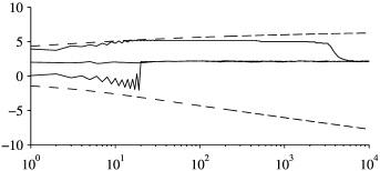
Figure 2: Trajectories of the estimate $\hat{\alpha}(\theta_{i})$ corresponding the PIMH-EM started from three different initial values for $\hat{\alpha}_{0}$. The dashed lines correspond to the boundaries induced to $\hat{\alpha}(\theta_{i})$ by $(\underline{\theta}_{i})_{i\geq 0}$ and $(\bar{\theta}_{i})_{i\geq 0}$. Notice the logarithmic scale on the $x$-axis (iterations).

5.5 Numerical experiment

We illustrate our algorithm briefly in practice in the setup of Proposition 5.8. We consider the same setting as Fort and Moulines [16]: we have $n=100$ simulated observations of the model of Section 5.2 with parameters $\alpha=2$, $\rho=0.4$ and $\sigma^{2}=1$.

We use the following projection sequences to control the sufficient statistic

$$\underline{\theta}_{i}:=\underline{c}\log^{\underline{\epsilon}-1}(i+2)\quad\mbox{and}\quad\bar{\theta}_{i}:=\bar{c}_{1}(i+2)^{\bar{c}_{2}/\log^{\bar{\epsilon}}(i+2)},$$

with the constants $\underline{c}=0.1m_{\theta}$, $\bar{c}_{1}=10m_{\theta}$, $\underline{\epsilon}=\bar{\epsilon}=0.1$ and $\bar{c}_{2}=1$, where $m_{\theta}:=n\exp(\frac{\sigma^{2}}{2(1-\rho^{2})})$ is the prior expectation of the sufficient statistic. The step size sequence parameters are $c_{\gamma}=6$, $c_{p}=3$ and $\gamma_{\eta}=\gamma_{p}=0.35$. The number of particles is set to $N=1000$.

Figure 2 shows the trajectories of the estimates $\hat{\alpha}(\theta_{i})$ for $10\mathord{,}000$ iterations of the algorithm starting from three different initial values $\hat{\alpha}_{0}\in\{0,2,4\}$. The final values of the estimates $\hat{\alpha}$ are within 2.10–2.16. The average acceptance rate during the runs varied between 46–72%. Notice the unstable initial behaviour of the estimates in Figure 2, which is controlled by the projections.

Appendix A Geometric ergodicity from drift condition

Before the proof of Proposition 3.11, we restate the result by Meyn and Tweedie [23] upon which the proof relies.

Theorem A.1 ((Meyn and Tweedie [23] Theorem 2.3))

Suppose Condition 3.10 holds. Then, for all $k\geq 0$ and $\|f\|_{V}<\infty$

$$\bigl{|}P_{s}^{k}(x,f)-\pi(f)\bigr{|}\leq V(x)(1+\gamma)\frac{\rho}{\rho-\vartheta}\rho^{k}\|f\|_{V}$$

for any $\rho>\vartheta=1-\tilde{M}^{-1}$, for

$$\tilde{M}=\frac{1}{(1-\check{\lambda})^{2}}\bigl{[}1-\check{\lambda}+\check{b}+\check{b}^{2}+\bar{\zeta}\bigl{(}\check{b}(1-\check{\lambda})+\check{b}^{2}\bigr{)}\bigr{]},$$

defined in terms of

$$\gamma=\delta^{-2}[4b+2\delta\lambda v],\qquad\check{\lambda}=(\lambda+\gamma)/(1+\gamma)<1\quad\mbox{and}\quad\check{b}=v+\gamma<\infty,$$

and the bound

$$\bar{\zeta}\leq\frac{4-\delta^{2}}{\delta^{5}}\biggl{(}\frac{b}{1-\lambda}\biggr{)}^{2}.$$

Proof of Proposition 3.11 Let us first consider the claim for $r=1$. Define first

$$\bar{\zeta}:=\bigl{(}4-\delta^{2}\bigr{)}\delta^{-5}b^{2}(1-\lambda)^{-2}\leq 4\delta^{-5}\bar{b}^{2}(1-\lambda)^{-2},$$

and observe that $\gamma:=\delta^{-2}[4b+2\delta\lambda v]\leq 6\delta^{-2}\bar{b}$. We also have

$$\check{\lambda}:=\frac{\lambda+\gamma}{1+\gamma}\leq\frac{\lambda+6\delta^{-2}\bar{b}}{1+6\delta^{-2}\bar{b}}\quad\mbox{implying}\quad\frac{1}{1-\check{\lambda}}\leq\frac{1+6\delta^{-2}\bar{b}}{1-\lambda}\leq\frac{7\delta^{-2}\bar{b}}{1-\lambda}.$$

We have also $\check{b}:=v+\gamma\leq 7\delta^{-2}\bar{b}$. Now, we can bound

$$\tilde{M} := \frac{1}{(1-\check{\lambda})^{2}}\bigl{[}1-\check{\lambda}+\check{b}+\check{b}^{2}+\bar{\zeta}\bigl{(}\check{b}(1-\check{\lambda})+\check{b}^{2}\bigr{)}\bigr{]}$$

$$\leq \frac{1}{(1-\check{\lambda})^{2}}\bar{\zeta}\bigl{(}5\check{b}^{2}\bigr{)}\leq 48\mbox{,}020(1-\lambda)^{-4}\delta^{-13}\bar{b}^{6}.$$

Now we can take $\rho_{1}:=1-[100\mbox{,}000(1-\lambda)^{-4}\delta^{-13}\bar{b}^{6}]^{-1}$ satisfying $\rho_{1}>1-\tilde{M}^{-1}/2$. Finally, the claim holds with $c_{1}^{*}=c^{*}:=336\mbox{,}140$ by setting

$$M_{1}:=(1+\gamma)\frac{\rho}{\rho-(1-\tilde{M}^{-1})}\leq(1+\gamma)2\tilde{M}\leq 336\mbox{,}140(1-\lambda)^{-4}\delta^{-15}\bar{b}^{7}.$$

Let us consider then the case $r\in(0,1)$. Observe first that by Jensen’s inequality

$$PV^{r}(x) \leq \bigl{(}PV(x)\bigr{)}^{r}\leq\lambda^{r}V^{r}(x)\qquad\mbox{for all }x\notin C,$$

$$PV^{r}(x) \leq \Bigl{(}\sup_{z\in C}V(z)+b\Bigr{)}^{r}\leq 2^{r}(v\vee b)^{r}\qquad\mbox{for all }x\in C.$$

That is, Condition 3.10 holds for $V^{r}$ with $\lambda_{r}:=\lambda^{r}$, $\bar{b}_{r}:=2\bar{b}^{r}$, and $v_{r}:=\sup_{x\in C}V^{r}(x)=(\sup_{x\in C}V(x))^{r}=v^{r}$. Because $t\mapsto t^{r}$ is concave, $\lambda^{r}\leq 1-r(1-\lambda)$ and so $(1-\lambda^{r})^{-1}\leq r^{-1}(1-\lambda)^{-1}$. We may take $c_{r}^{*}:=(2r^{-1})^{4}c^{*}$.

Appendix B Noise condition for convergence theorem

Proof of Theorem 4.4 We give only the required modifications to the proof of Theorem 3.3 regarding (13). First, by symbolically substituting $\nabla{w}\equiv 1$, it is sufficient to show that claim holds for the following four terms in turn:

$$R_{m,n}^{1} := \sum_{i=m}^{n}\Gamma_{i+1}\bigl{(}g_{\theta_{i}}(X_{i+1})-P_{\theta_{i}}g_{\theta_{i}}(X_{i})\bigr{)}\mathbb{I}\bigl{\{}A_{\mathcal{R}}^{i}\bigr{\}},$$

$$R_{m,n}^{2} := \sum_{i=m}^{n}\Gamma_{i+1}\bigl{(}P_{\theta_{i}}g_{\theta_{i}}(X_{i})-P_{\theta_{i-1}}g_{\theta_{i-1}}(X_{i})\bigr{)}\mathbb{I}\bigl{\{}A_{\mathcal{R}}^{i}\bigr{\}},$$

$$R_{m,n}^{4} := \bigl{(}\Gamma_{m}P_{\theta_{m-1}}g_{\theta_{m-1}}(X_{m})-\Gamma_{n+1}P_{\theta_{n}}g_{\theta_{n}}(X_{n+1})\bigr{)}\mathbb{I}\bigl{\{}A_{\mathcal{R}}^{n}\bigr{\}},$$

$$R_{m,n}^{5} := \sum_{i=m}^{n}(\Gamma_{i+1}-\Gamma_{i})P_{\theta_{i-1}}g_{\theta_{i-1}}(X_{i})\mathbb{I}\bigl{\{}A_{\mathcal{R}}^{i-1}\bigr{\}}.$$

The first term $R_{m,n}^{1}$ is a martingale, so by Doob’s inequality, (24) and (25),

$$\Bigl{(}\mathbb{E}_{\theta,x}\Bigl{[}\sup_{n\geq m}\bigl{|}R_{m,n}^{1}\bigr{|}\Bigr{]}\Bigr{)}^{2} \leq C\sum_{i=m}^{\infty}\mathbb{E}_{\theta,x}\bigl{[}\Gamma_{i+1}^{2}\bigl{|}g_{\theta_{i}}(X_{i+1})-P_{\theta_{i}}g_{\theta_{i}}(X_{i})\bigr{|}^{2}\mathbb{I}\bigl{\{}A_{\mathcal{R}}^{i}\bigr{\}}\bigr{]}$$

$$\leq CV^{2\beta_{g}}(x)\sum_{i=m}^{\infty}\mathbb{E}\bigl{[}\Gamma_{i+1}^{2}\bigr{]}\mathop{\hbox to30.0pt{\rightarrowfill}}^{m\to\infty}0.$$

The claim for the second term is implied directly by (26). For the term $R_{m,n}^{4}$, it is enough to observe that

$$\mathbb{E}_{\theta,x}\Bigl{[}\sup_{n\geq m}\bigl{(}R_{m,n}^{4}\bigr{)}^{2}\Bigr{]}\leq 4\sum_{i=m}^{\infty}\mathbb{E}\bigl{[}\Gamma_{i}^{2}\bigr{]}\mathbb{E}_{\theta,x}\bigl{[}\bigl{|}P_{\theta_{i-1}}g_{\theta_{i-1}}(X_{i})\bigr{|}^{2}\mathbb{I}\bigl{\{}A_{\mathcal{R}}^{i-1}\bigr{\}}\bigr{]}\leq CV^{2\beta_{g}}(x)\sum_{i=m}^{\infty}\mathbb{E}\bigl{[}\Gamma_{i}^{2}\bigr{]}.$$

Finally, we may employ Lemma 3.4 for $R_{m,n}^{5}$ with $U_{i}:=\Gamma_{i}$ and $B_{i-1}\break:=|P_{\theta_{i-1}}g_{\theta_{i-1}}(X_{i})|\mathbb{I}\{A_{\mathcal{R}}^{i-1}\}$ because $\mathbb{E}_{\theta,x}[|B_{i-1}|]\leq CV^{\beta_{g}}(x)$ and $\mathbb{E}_{\theta,x}[B_{i-1}^{2}]\leq CV^{2\beta_{g}}(x)$.

Appendix C Geometric ergodicity of IMH

We provide here quantitative bounds for the ergodicity constants for independent Metropolis–Hastings kernels. To our knowledge, the results here are new, and can be useful also in other settings.

Recall that the independent Metropolis–Hastings kernel with target density $\pi$ and proposal density $q$ on space $\mathsf{X}\subset\mathbb{R}^{d}$ is defined as

$$P(x,A):=\int_{A}\alpha(x,y)q(y)\,\mathrm{d}y+\mathbb{I}\{x\in A\}\biggl{(}1-\int_{\mathsf{X}}\alpha(x,y)q(y)\,\mathrm{d}y\biggr{)}$$

for all $x\in\mathsf{X}$ and measurable $A\subset\mathsf{X}$, where the acceptance probability $\alpha(x,y)$ is defined as

$$\alpha(x,y):=\min\biggl{\{}1,\frac{\pi(y)/q(y)}{\pi(x)/q(x)}\biggr{\}}.$$

Proposition C.1

Assume $P$ is the independent Metropolis–Hastings kernel with target density $\pi$ and proposal density $q$ satisfying $\epsilon:=\inf_{x\in\mathsf{X}}q(x)/\pi(x)>0$. Let $V\mathchoice{\nobreak\,\colon}{\nobreak\,\colon}{\nobreak\,\colon\;}{\nobreak\,\colon\;}\mathsf{X}\to[1,\infty)$ be a function with $q(V)<\infty$. Then,

1. [(ii)]

2. the drift inequality

   $$PV(x)\leq\rho V(x)+q(V)\qquad\mbox{for all }x\in\mathsf{X}$$

   holds with the constant $\rho:=1-\epsilon$, and

3. the following bound holds for any measurable function $f\mathchoice{\nobreak\,\colon}{\nobreak\,\colon}{\nobreak\,\colon\;}{\nobreak\,\colon\;}\mathsf{X}\to\mathbb{R}^{d}$ with $\|f\|_{V}:=\sup_{x\in\mathsf{X}}|f(x)|/V(x)<\infty$, all $k\geq 1$ and all $x\in\mathsf{X}$

   $$\bigl{|}P^{k}f(x)-\pi(f)\bigr{|}\leq kM(1-\epsilon)^{k}\|f\|_{V}V(x),$$

   where the constant $M=q(V)[1+\epsilon^{-1}+(1-\epsilon)^{-1}]$.

Proof.

Denote by $r(x):=\pi(x)/q(x)$ so that $\alpha(x,y)=\min\{1,r(x)/r(y)\}$ and compute

$$\frac{PV(x)}{V(x)}-1=\frac{\int V(y)\alpha(x,y)q(y)\,\mathrm{d}y}{V(x)}-\int\min\bigl{\{}r^{-1}(y),r^{-1}(x)\bigr{\}}\pi(y)\,\mathrm{d}y\leq\frac{q(V)}{V(x)}-\epsilon.$$

This readily implies (i).

Observe then that for any measurable $A\subset\mathsf{X}$, the following uniform minorisation inequality holds

$$P(x,A)\geq\int_{A}\alpha(x,y)q(y)\,\mathrm{d}y\geq\epsilon\pi(A).$$

By this inequality, one can define a Markov kernel $Q(x,A):=(1-\epsilon)^{-1}(P(x,A)-\epsilon\pi(A))$. By (i), we have $QV(x)\leq(1-\epsilon)^{-1}(\rho V(x)+q(V))=V(x)+(1-\epsilon)^{-1}q(V)$ so by induction we obtain

$$Q^{k}V(x)\leq V(x)+k(1-\epsilon)^{-1}q(V).$$

Observe that for any probability measure $\nu$ with $\nu(V)<\infty$, one has $\nu(|f|)\leq\|f\|_{V}\nu(V)$, and that

$$\pi(V)=\int\frac{\pi(x)}{q(x)}V(x)q(x)\,\mathrm{d}x\leq\epsilon^{-1}q(V).$$

Note that $\pi Q=\pi$, whence by denoting $\Pi(x,\cdot):=\pi(\cdot)$ one can compute for any $k\geq 1$

$$\bigl{|}P^{k}f(x)-\pi(f)\bigr{|} = \bigl{|}(P-\Pi)P^{k-1}f(x)\bigr{|}=(1-\epsilon)\bigl{|}(Q-\Pi)P^{k-1}f(x)\bigr{|}$$

$$= (1-\epsilon)\bigl{|}QP^{k-1}f(x)-\pi(f)\bigr{|}={\cdots}=(1-\epsilon)^{k}\bigl{|}Q^{k}f(x)-\pi(f)\bigr{|}$$

$$\leq (1-\epsilon)^{k}\bigl{(}V(x)+k(1-\epsilon)^{-1}+\epsilon^{-1}\bigr{)}\|f\|_{V}q(V),$$

establishing (ii). ∎

Corollary C.2

In Proposition C.1, the bound (ii) can be replaced with the following

$$\bigl{|}P^{k}f(x)-\pi(f)\bigr{|}\leq M^{\prime}(1-\zeta\epsilon)^{k}\|f\|_{V}V(x),$$

where $\zeta\in(0,1)$ can be chosen arbitrarily and where

$$M^{\prime}=\frac{M}{\mathrm{e}}\biggl{[}\log\biggl{(}\frac{1-\zeta\epsilon}{1-\epsilon}\biggr{)}\biggr{]}^{-1}.$$

If $\epsilon\leq 1/2$, then $M^{\prime}$ can be taken as $M^{\prime}=2M[\mathrm{e}(1-\zeta)\epsilon]^{-1}$.

Proof.

From Proposition C.1, we obtain

$$\bigl{|}P^{k}f(x)-\pi(f)\bigr{|} \leq kM(1-\epsilon)^{k}\|f\|_{V}V(x)$$

$$\leq M^{\prime}(1-\zeta\epsilon)^{k}\|f\|_{V}V(x),$$

with

$$M^{\prime}:=M\sup_{k\geq 1}k\biggl{(}\frac{1-\epsilon}{1-\zeta\epsilon}\biggr{)}^{k}\leq\frac{M}{\mathrm{e}}\biggl{[}\log\biggl{(}\frac{1-\zeta\epsilon}{1-\epsilon}\biggr{)}\biggr{]}^{-1},$$

since by a straightforward calculation one obtains for any $a\in(0,1)$ that $\sup_{x>0}xa^{x}=(\mathrm{e}\log(1/a))^{-1}$. Suppose then that $\epsilon\leq 1/2$ and notice that for any $h>0$ one has $\log(1+h)\geq h-\frac{1}{2}h^{2}$ and so

$$\log\biggl{(}\frac{1-\zeta\epsilon}{1-\epsilon}\biggr{)}\geq\frac{(1-\zeta)\epsilon}{1-\epsilon}\biggl{(}1-\frac{1}{2}\frac{(1-\zeta)\epsilon}{1-\epsilon}\biggr{)}\geq\frac{1}{2}(1-\zeta)\epsilon.$$

∎

Appendix D Nomenclature

• $\alpha_{w}$ in Condition 2.1, page 2.1, related to the growth of $\sup_{\theta\in\mathcal{R}_{i}}|\nabla w(\theta)|$.

• $\alpha_{H},\beta_{H}$ in Condition 3.1, page 3.1, characterise $\sup_{\theta\in\mathcal{R}_{i}}|H(\theta,x)|$.

• $\alpha_{V},\beta_{V}$ in Condition 3.1, page 3.1, characterise $\mathbb{E}_{\theta,x}[V(X_{i})]$.

• $\alpha_{g},\beta_{g}$ in Condition 3.1, page 3.1, characterise $\sup_{\theta\in\mathcal{R}_{i}}[|g_{\theta}(x)|+|P_{\theta}g_{\theta}(x)|]$.

• $\beta_{D}$ in Condition 3.12, page 3.12, characterises the Hölder continuity of $\|P_{\theta}f-P_{\theta^{\prime}}f\|_{V^{r}}$.

• $\alpha_{\Delta},\beta_{\Delta}$ in Condition 3.15, page 3.15, characterise the size of $\sup_{(\theta,\theta^{\prime})\in\mathcal{R}_{i}^{2}}\|H(\theta,\cdot)-H(\theta^{\prime},\cdot)\|_{V^{\beta_{H}}}$.

• $\alpha_{M}$ and $\alpha_{\rho}$ are defined in Condition 3.8, page 3.8, and characterise the loss of ergodicity through the growth of geometric ergodicity constants $\sup_{\theta\in\mathcal{R}_{i}}M_{\theta,r}$ and $\sup_{\theta\in\mathcal{R}_{i}}(1-\rho_{\theta,r})^{-1}$, respectively.

References

- [1] {barticle}[mr] \bauthor\bsnmAndradóttir, \bfnmSigrún\binitsS. (\byear1995). \btitleA stochastic approximation algorithm with varying bounds. \bjournalOper. Res. \bvolume43 \bpages1037–1048. \biddoi=10.1287/opre.43.6.1037, issn=0030-364X, mr=1488889 \bptokimsref\endbibitem
- [2] {barticle}[mr] \bauthor\bsnmAndrieu, \bfnmChristophe\binitsC., \bauthor\bsnmDoucet, \bfnmArnaud\binitsA. &\bauthor\bsnmHolenstein, \bfnmRoman\binitsR. (\byear2010). \btitleParticle Markov chain Monte Carlo methods. \bjournalJ. R. Stat. Soc. Ser. B Stat. Methodol. \bvolume72 \bpages269–342. \biddoi=10.1111/j.1467-9868.2009.00736.x, issn=1369-7412, mr=2758115 \bptnotecheck related \bptokimsref\endbibitem
- [3] {barticle}[mr] \bauthor\bsnmAndrieu, \bfnmChristophe\binitsC. &\bauthor\bsnmMoulines, \bfnmÉric\binitsÉ. (\byear2006). \btitleOn the ergodicity properties of some adaptive MCMC algorithms. \bjournalAnn. Appl. Probab. \bvolume16 \bpages1462–1505. \biddoi=10.1214/105051606000000286, issn=1050-5164, mr=2260070 \bptokimsref\endbibitem
- [4] {barticle}[mr] \bauthor\bsnmAndrieu, \bfnmChristophe\binitsC., \bauthor\bsnmMoulines, \bfnmÉric\binitsÉ. &\bauthor\bsnmPriouret, \bfnmPierre\binitsP. (\byear2005). \btitleStability of stochastic approximation under verifiable conditions. \bjournalSIAM J. Control Optim. \bvolume44 \bpages283–312. \biddoi=10.1137/S0363012902417267, issn=0363-0129, mr=2177157 \bptokimsref\endbibitem
- [5] {btechreport}[author] \bauthor\bsnmAndrieu, \bfnmChristophe\binitsC., \bauthor\bsnmMoulines, \bfnmÉric\binitsÉ. &\bauthor\bsnmVolkov, \bfnmStanislav\binitsS. (\byear2004). \btitleConvergence of stochastic approximation for Lyapunov stable dynamics: A proof from first principles \btypeTechnical report. \bptokimsref\endbibitem
- [6] {bmisc}[author] \bauthor\bsnmAndrieu, \bfnmChristophe\binitsC., \bauthor\bsnmTadić, \bfnmVladislav B.\binitsV.B. &\bauthor\bsnmVihola, \bfnmMatti\binitsM. (\byear2012). \btitleOn the stability of controlled Markov chains and its applications to stochastic approximation with Markovian dynamic. \bnoteAvailable at arXiv:\arxivurl1205.4181v1. \bptokimsref\endbibitem
- [7] {bincollection}[mr] \bauthor\bsnmBenaïm, \bfnmMichel\binitsM. (\byear1999). \btitleDynamics of stochastic approximation algorithms. In \bbooktitleSéminaire de Probabilités, XXXIII. \bseriesLecture Notes in Math. \bvolume1709 \bpages1–68. \blocationBerlin: \bpublisherSpringer. \biddoi=10.1007/BFb0096509, mr=1767993 \bptokimsref\endbibitem
- [8] {bbook}[mr] \bauthor\bsnmBenveniste, \bfnmAlbert\binitsA., \bauthor\bsnmMétivier, \bfnmMichel\binitsM. &\bauthor\bsnmPriouret, \bfnmPierre\binitsP. (\byear1990). \btitleAdaptive Algorithms and Stochastic Approximations. \bseriesApplications of Mathematics (New York) \bvolume22. \blocationBerlin: \bpublisherSpringer. \bnoteTranslated from the French by Stephen S. Wilson. \bidmr=1082341 \bptokimsref\endbibitem
- [9] {bbook}[mr] \bauthor\bsnmBorkar, \bfnmVivek S.\binitsV.S. (\byear2008). \btitleStochastic Approximation: A Dynamical Systems Viewpoint. \blocationCambridge: \bpublisherCambridge Univ. Press. \bidmr=2442439 \bptokimsref\endbibitem
- [10] {barticle}[mr] \bauthor\bsnmChan, \bfnmK. S.\binitsK.S. &\bauthor\bsnmLedolter, \bfnmJohannes\binitsJ. (\byear1995). \btitleMonte Carlo EM estimation for time series models involving counts. \bjournalJ. Amer. Statist. Assoc. \bvolume90 \bpages242–252. \bidissn=0162-1459, mr=1325132 \bptokimsref\endbibitem
- [11] {bbook}[mr] \bauthor\bsnmChen, \bfnmHan-Fu\binitsH.-F. (\byear2002). \btitleStochastic Approximation and Its Applications. \bseriesNonconvex Optimization and Its Applications \bvolume64. \blocationDordrecht: \bpublisherKluwer Academic. \bidmr=1942427 \bptokimsref\endbibitem
- [12] {barticle}[mr] \bauthor\bsnmChen, \bfnmHan Fu\binitsH.F., \bauthor\bsnmLei, \bfnmGuo\binitsG. &\bauthor\bsnmGao, \bfnmAi Jun\binitsA.J. (\byear1988). \btitleConvergence and robustness of the Robbins–Monro algorithm truncated at randomly varying bounds. \bjournalStochastic Process. Appl. \bvolume27 \bpages217–231. \biddoi=10.1016/0304-4149(87)90039-1, issn=0304-4149, mr=0931029 \bptokimsref\endbibitem
- [13] {barticle}[mr] \bauthor\bsnmChen, \bfnmHan Fu\binitsH.F. &\bauthor\bsnmZhu, \bfnmYun Min\binitsY.M. (\byear1986). \btitleStochastic approximation procedures with randomly varying truncations. \bjournalSci. Sinica Ser. A \bvolume29 \bpages914–926. \bidissn=0253-5831, mr=0869196 \bptokimsref\endbibitem
- [14] {barticle}[mr] \bauthor\bsnmDelyon, \bfnmBernard\binitsB., \bauthor\bsnmLavielle, \bfnmMarc\binitsM. &\bauthor\bsnmMoulines, \bfnmEric\binitsE. (\byear1999). \btitleConvergence of a stochastic approximation version of the EM algorithm. \bjournalAnn. Statist. \bvolume27 \bpages94–128. \biddoi=10.1214/aos/1018031103, issn=0090-5364, mr=1701103 \bptokimsref\endbibitem
- [15] {bmisc}[author] \bauthor\bsnmDonnet, \bfnmSophie\binitsS. &\bauthor\bsnmSamson, \bfnmAdeline\binitsA. (\byear2011). \btitleEM algorithm coupled with particle filter for maximum likelihood parameter estimation of stochastic differential mixed-effect models. \bhowpublishedTechnical Report hal-00519576 v2, Universite Paris Descartes MAP5. \bptokimsref\endbibitem
- [16] {barticle}[mr] \bauthor\bsnmFort, \bfnmGersende\binitsG. &\bauthor\bsnmMoulines, \bfnmEric\binitsE. (\byear2003). \btitleConvergence of the Monte Carlo expectation maximization for curved exponential families. \bjournalAnn. Statist. \bvolume31 \bpages1220–1259. \biddoi=10.1214/aos/1059655912, issn=0090-5364, mr=2001649 \bptokimsref\endbibitem
- [17] {barticle}[mr] \bauthor\bsnmFort, \bfnmG.\binitsG., \bauthor\bsnmMoulines, \bfnmE.\binitsE., \bauthor\bsnmRoberts, \bfnmG. O.\binitsG.O. &\bauthor\bsnmRosenthal, \bfnmJ. S.\binitsJ.S. (\byear2003). \btitleOn the geometric ergodicity of hybrid samplers. \bjournalJ. Appl. Probab. \bvolume40 \bpages123–146. \bidissn=0021-9002, mr=1953771 \bptokimsref\endbibitem
- [18] {barticle}[mr] \bauthor\bsnmJarner, \bfnmSøren Fiig\binitsS.F. &\bauthor\bsnmHansen, \bfnmErnst\binitsE. (\byear2000). \btitleGeometric ergodicity of Metropolis algorithms. \bjournalStochastic Process. Appl. \bvolume85 \bpages341–361. \biddoi=10.1016/S0304-4149(99)00082-4, issn=0304-4149, mr=1731030 \bptokimsref\endbibitem
- [19] {barticle}[mr] \bauthor\bsnmKamal, \bfnmSameer\binitsS. (\byear2012). \btitleStabilization of stochastic approximation by step size adaptation. \bjournalSystems Control Lett. \bvolume61 \bpages543–548. \biddoi=10.1016/j.sysconle.2012.02.005, issn=0167-6911, mr=2910330 \bptokimsref\endbibitem
- [20] {bbook}[mr] \bauthor\bsnmKushner, \bfnmHarold J.\binitsH.J. &\bauthor\bsnmClark, \bfnmDean S.\binitsD.S. (\byear1978). \btitleStochastic Approximation Methods for Constrained and Unconstrained Systems. \bseriesApplied Mathematical Sciences \bvolume26. \blocationNew York: \bpublisherSpringer. \bidmr=0499560 \bptokimsref\endbibitem
- [21] {bbook}[mr] \bauthor\bsnmKushner, \bfnmHarold J.\binitsH.J. &\bauthor\bsnmYin, \bfnmG. George\binitsG.G. (\byear2003). \btitleStochastic Approximation and Recursive Algorithms and Applications, \bedition2nd ed. \bseriesApplications of Mathematics (New York): Stochastic Modelling and Applied Probability \bvolume35. \blocationNew York: \bpublisherSpringer. \bidmr=1993642 \bptokimsref\endbibitem
- [22] {barticle}[mr] \bauthor\bsnmMengersen, \bfnmK. L.\binitsK.L. &\bauthor\bsnmTweedie, \bfnmR. L.\binitsR.L. (\byear1996). \btitleRates of convergence of the Hastings and Metropolis algorithms. \bjournalAnn. Statist. \bvolume24 \bpages101–121. \biddoi=10.1214/aos/1033066201, issn=0090-5364, mr=1389882 \bptokimsref\endbibitem
- [23] {barticle}[mr] \bauthor\bsnmMeyn, \bfnmSean P.\binitsS.P. &\bauthor\bsnmTweedie, \bfnmR. L.\binitsR.L. (\byear1994). \btitleComputable bounds for geometric convergence rates of Markov chains. \bjournalAnn. Appl. Probab. \bvolume4 \bpages981–1011. \bidissn=1050-5164, mr=1304770 \bptokimsref\endbibitem
- [24] {barticle}[mr] \bauthor\bsnmRoberts, \bfnmGareth O.\binitsG.O. &\bauthor\bsnmRosenthal, \bfnmJeffrey S.\binitsJ.S. (\byear2007). \btitleCoupling and ergodicity of adaptive Markov chain Monte Carlo algorithms. \bjournalJ. Appl. Probab. \bvolume44 \bpages458–475. \biddoi=10.1239/jap/1183667414, issn=0021-9002, mr=2340211 \bptokimsref\endbibitem
- [25] {barticle}[mr] \bauthor\bsnmSaksman, \bfnmEero\binitsE. &\bauthor\bsnmVihola, \bfnmMatti\binitsM. (\byear2010). \btitleOn the ergodicity of the adaptive Metropolis algorithm on unbounded domains. \bjournalAnn. Appl. Probab. \bvolume20 \bpages2178–2203. \biddoi=10.1214/10-AAP682, issn=1050-5164, mr=2759732 \bptokimsref\endbibitem
- [26] {barticle}[mr] \bauthor\bsnmSharia, \bfnmT.\binitsT. (\byear1997). \btitleTruncated recursive estimation procedures. \bjournalProc. A. Razmadze Math. Inst. \bvolume115 \bpages149–159. \bidissn=1512-0007, mr=1639120 \bptokimsref\endbibitem
- [27] {bmisc}[author] \bauthor\bsnmSharia, \bfnmTeo\binitsT. (\byear2011). \btitleTruncated stochastic approximation with moving bounds: Convergence. \bnoteAvailable at arXiv:\arxivurl1101.0031v3. \bptokimsref\endbibitem
- [28] {barticle}[mr] \bauthor\bsnmTadić, \bfnmVladislav\binitsV. (\byear1998). \btitleStochastic approximation with random truncations, state-dependent noise and discontinuous dynamics. \bjournalStochastics Stochastics Rep. \bvolume64 \bpages283–326. \bidissn=1045-1129, mr=1709288 \bptokimsref\endbibitem
- [29] {barticle}[mr] \bauthor\bsnmVihola, \bfnmMatti\binitsM. (\byear2011). \btitleOn the stability and ergodicity of adaptive scaling Metropolis algorithms. \bjournalStochastic Process. Appl. \bvolume121 \bpages2839–2860. \biddoi=10.1016/j.spa.2011.08.006, issn=0304-4149, mr=2844543 \bptokimsref\endbibitem
- [30] {barticle}[mr] \bauthor\bsnmYounes, \bfnmLaurent\binitsL. (\byear1999). \btitleOn the convergence of Markovian stochastic algorithms with rapidly decreasing ergodicity rates. \bjournalStochastics Stochastics Rep. \bvolume65 \bpages177–228. \bidissn=1045-1129, mr=1687636 \bptokimsref\endbibitem
- [31] {barticle}[mr] \bauthor\bsnmZeger, \bfnmScott L.\binitsS.L. (\byear1988). \btitleA regression model for time series of counts. \bjournalBiometrika \bvolume75 \bpages621–629. \biddoi=10.1093/biomet/75.4.621, issn=0006-3444, mr=0995107 \bptokimsref\endbibitem