Stellar population models in the UV: I. Characterisation of the New Generation Stellar Library

Abstract

Context. The spectral predictions of stellar population models are not as accurate in the ultra-violet (UV) as in the optical wavelength domain. One of the reasons is the lack of high-quality stellar libraries. The New Generation Stellar Library (NGSL), recently released, represents a significant step towards the improvement of this situation.

Aims. To prepare NGSL for population synthesis, we determined the atmospheric parameters of its stars, we assessed the precision of the wavelength calibration and characterised its intrinsic resolution. We also measured the Galactic extinction for each of the NGSL stars.

Methods. For our analyses we used ULySS, a full spectrum fitting package, fitting the NGSL spectra against the MILES interpolator.

Results. We find that the wavelength calibration is precise up to 0.1 px, after correcting a systematic effect in the optical range. The spectral resolution varies from 3 Å in the UV to 10 Å in the near-infrared (NIR), corresponding to a roughly constant reciprocal resolution $R=\lambda/\delta\lambda\approx 1000$ and an instrumental velocity dispersion $\sigma_{ins}\approx 130$ km s^-1. We derived the atmospheric parameters homogeneously. The precision for the FGK stars is 42 K, 0.24 and 0.09 dex for T_eff, $log$g and [Fe/H], respectively. The corresponding mean errors are 29 K, 0.50 and 0.48 dex for the M stars, and for the OBA stars they are 4.5 percent, 0.44 and 0.18 dex. The comparison with the literature shows that our results are not biased.

1 Introduction

The stellar libraries are collections of spectra that share identical spectral coverage and resolution. They have several important applications: They are used as references to classify stars and to determine their atmospheric parameters (e.g. Wu et al.  2011b, and the reference therein), as templates to recover the line-of-sight velocity distribution of galaxies (e.g. Cappellari & Emsellem  2004), or to calibrate photometry (see Bessell  2005, for a review). They are one of the critical ingredients in the stellar population synthesis (e.g. Vazdekis et al.  2010). To produce high-quality stellar population in the blue is the goal of this series of papers.

The stellar libraries can be theoretical or observational. The theoretical libraries can, in principle, be computed for any value of temperature, gravity, metallicity and detailed chemical composition, and the resolution is essentially limited by the computing power (e.g. Kurucz  1979; Hauschildt et al.  2003; Palacios et al.  2010). They would be the ideal references if they were able to reproduce the observations accurately. In fact, the physical approximations (1D, LTE, convection, …) and the lack of complete databases of atomic and molecular transition result in discrepancies between these stellar models and observations (Martins & Coelho  2007; Prugniel et al.  2011; Beifiori et al.  2011). The observational libraries, on the other side, have the advantage to be assembled from real stars, but they suffer from instrumental limitations (finite resolution) and limited atmospheric parameter coverage. Because these libraries are constructed from Galactic stars, they are bound to the chemical composition found in the Galaxy, and more specifically that of the solar neighbourhood. It is possible to combine the observed and theoretical libraries to predict the differential effect of changing some physical ingredients. These semi-empirical libraries were used to extend the range of the parameter space (Prugniel et al.  2011) or to compute the effect of a variable abundance of $\alpha$-elements in models of stellar populations (Cervantes et al.  2007; Prugniel et al.  2007a; Walcher et al.  2009).

The most important property of the stellar libraries is the coverage of the atmospheric parameters, such as effective temperature, gravity, metallicity. Recently, the detailed abundances are beginning to be considered as important parameters, too. Other properties to be considered are the spectral resolution, the wavelength coverage, the flux, and the wavelength calibration of the spectra. Fortunately, we have optical libraries that cover the parameter space reasonably well: ELODIE (Prugniel & Soubiran  2001; Prugniel et al.  2007b), CFLIB (Valdes et al.  2004), and MILES (Sánchez-Blázquez et al.  2006). These empirical libraries have a fair spectral resolution ($\lambda/\Delta\lambda=R\sim 2000-10000$) that is compatible with the resolution of the most widely used optical spectrographs for galactic studies, and they have a good flux calibration (except CFLIB, Bruzual A.  2007). They are built from normal stars in all luminosity classes and spectral types from O to M. They cover a wide range in metallicities ($-3.0\lesssim{\rm[Fe/H]}\lesssim 1.0$). The stars in these three libraries, as in any other empirical library, have the abundance pattern of the solar neighbourhood (see Wheeler et al.  1989, for a review).

None of these three libraries extend further blue-ward than 3500 Å. The importance of the UV as a gate to understand the physics of the stellar systems was recognised back in the 1980s (e.g. Faber  1983). In particular, the UV is irreplaceable to characterise the metallicity and the star-formation history (SFH) of young populations, to study the enhancement of $\alpha$-elements or the contribution of blue horizontal branch stars to the integrated fluxes. It is also of prime importance studying distant galaxies whose restframe UV is observed in the optical, where the current instrumentation is most developed.

In a simple stellar population (SSP) the blue wavelengths are predominantly sensitive to the hottest stars. At any age greater than 10 Myr, those are the dwarfs at the main-sequence turn-off. After $\sim$1 Gyr of evolution, the He-burning stars may become bluer (hotter) than the RR Lyrae pulsating stars and populate the so-called blue-horizontal branch (BHB). Together with the blue stragglers (BS, low-mass, main-sequence stars with excessive blue colours) they may have an important contribution to the integrated spectra (Lee et al.  2002; Cenarro et al.  2008) and mimic young populations (e.g. Maraston & Thomas  2000; Koleva et al.  2008; Ocvirk  2010; Percival & Salaris  2011). Our ability to distinguish between the real young stars and these exotic populations relies on their different contribution to the different parts of the spectral energy distribution (SED). Thus, combining optical and UV data can lift the degeneracy (Rose  1984; Schiavon et al.  2004; Percival & Salaris  2011).

Blue-horizontal branch stars and blue stragglers are frequently observed in Galactic clusters and were also detected in Local Group galaxies (e.g. Mapelli et al.  2007). The presence of the BHB and BS is connected with some properties of the populations (e.g. the metallicity for the BHB) but may also be related with the environment and with some large scale properties of the host systems. Therefore, the ability to distinguish these stars in integrated spectra would be a major step toward the understanding for the genesis and evolution of stellar systems.

It has been shown that the effects of $\alpha$-elements enhanced partition are emphasised blue-ward, both in stars (e.g. Cassisi et al.  2004) and in stellar populations (Coelho et al.  2005). Thus, the blue spectral range should provide us with more diagnostic indices to better constrain the galactic star-formation histories (Serven et al.  2011).

The first attempts to gather a UV library that covered the MK sequence were made by Wu et al. (1983) and Fanelli et al. (1992) with observations from the International Ultraviolet Explorer (IUE). This library has a resolution of 7 Å and contains 218 stars of essentially solar metallicity. Still, this first UV library is quite limited compared to its modern optical counterparts. With the new generation stellar library (NGSL, Gregg et al. 2006) the gap between the optical and UV libraries begins to narrow.

The New Generation Spectral Library is a major step towards the modelling of the stellar populations in the UV. It was observed with the Hubble Space Telescope Imaging Spectrograph (STIS) and consists of 374 stars with metallicities between -2.0 dex and 0.5 dex. As its optical counterparts it contains normal stars from O to M spectral types in all luminosity classes. Its wavelength coverage from 0.2 to 1.0 $\mu$m is the widest available amongst the observational libraries at this resolution, though it does not go as far in the UV as IUE and misses Ly$\alpha$. Its spectral resolution is R$\sim$1000. The stars of the NGSL were rigorously chosen to have a good coverage in the space of atmospheric parameters. Heap & Lindler (2010) measured the atmospheric parameters for most NGSL stars using ATLAS9 model atmospheres (Castelli & Kurucz  2004) as templates (46 stars, i. e. $12$ percent of the sample, miss one or more parameters).

In order to implement this library in population models, its characteristics have to be assessed accurately. This is the goal of the present paper. In Sect. 2 we present the data, while in Sect. 3 we present our methodology. In Sect. 4 we characterise the line-spread function (LSF) of the NGSL. In Sect. 5 we derive the atmospheric parameters homogeneously and compare them with the literature. In Sect. 6 we measure the spectroscopic Galactic extinction of the stars. Finally, our conclusions and prospects are presented in Sect. 7.

2 The NGSL spectra

The NGSL stars were observed with STIS on-board HST with three different gratings (G230LB, G430L and G750L), overlapping at 2990-3060 Å and 5500-5650 Å (Gregg et al.  2006). The final spectra cover the wavelength range from $\sim$0.2 to $\sim$1.0 $\mu$m (slightly different from star to star) and have a resolution of R$\sim$1000. The flux-calibration reaches a precision of 3 percent (Heap & Lindler  2009). The spectra are calibrated in air wavelengths, with sampling varying as follows: 1.373 Å/px ($\lambda\lambda 1675-3060\,\AA$ or 165km s^-1at 2500 Å), 2.744 Å/px ($\lambda\lambda 3060-5650\,\AA$ or 205km s^-1at 4000 Å), 4.878 Å/px ($\lambda\lambda 5650-10196\,\AA$ or 183km s^-1at 8000 Å). Details about the data reduction can be found in http://archive.stsci.edu/pub/hlsp/stisngsl/aaareadme.pdf. We downloaded version 2 of the reduced data.

The stars were chosen to sample four metallicity groups, roughly 150 stars in each bin: [Fe/H]$<-1.5$; $-1.5<{\rm[Fe/H]}<-0.5$; $-0.3<{\rm[Fe/H]}<+0.1$; $+0.2<{\rm[Fe/H]}$. The targeted sample included 600 stars. Unfortunately, about 200 stars were not observed owing to the failure of STIS in 2004. The released library lacks some hot- and low-metallicity stars, but is well-suited to model intermediate- and old-aged stellar populations.

3 Methodology

We applied a full spectrum fitting approach to characterise the NGSL spectra and to infer the stellar parameters. For this purpose we employed the ULySS package (Koleva et al.  2009). We followed the approach used in Wu et al. (2011b), Prugniel et al. (2011), and Wu et al. (2011a) to derive (i) the LSF to describe the intrinsic resolution and its variation with wavelength, (ii) the atmospheric parameters of the stars, and (iii) the Galactic extinction on the line-of-sight of each star.

3.1 Spectral fitting

ULySS performs a parametric minimisation of the squared differences between an observation and a linear combination of non-linear models as

$$Obs(\lambda)=P_{n}(\lambda)\times\bigg{(} G(v_{sys},\sigma)$$

$$\otimes\sum_{i=0}^{i=k}W_{i}\,\,{\rm CMP}_{i}\,(a_{1},a_{2},...,\lambda)\bigg{)},$$ (1)

where $Obs(\lambda)$ is the observed one-dimensional spectrum function of the wavelength ($\lambda$), sampled in $log\lambda$; $P_{n}$ is a multiplicative polynomial of degree $n$; and $G(v_{res},\sigma)$ is a Gaussian broadening function parameterised by the residual velocity $v_{res}$, and the dispersion $\sigma$ (see the discussion in Sect. 4). The ${\rm CMP}_{i}$ are $k$ non-linear functions of any number of parameters, figuring the physical model. Their weights $W_{i}$ can be constrained (to be positive in the present case).

3.2 Applications

Here we will use three different specific cases of Eq. 1. First, to determine the broadening by comparing the stars in common between NGSL and a reference library, we used a single component that consists in a template spectrum (i.e. no non-linear parameter). Eq. 1 degenerates to

$$Obs(\lambda)=P_{n}(\lambda)\times G(v_{sys},\sigma)\otimes S(\lambda),$$ (2)

where $S(\lambda)$ is the template spectrum.

Second, to determine the broadening with respect to a theoretical library, we used a positive linear combination of spectra taken from a grid.

$$Obs(\lambda)=P_{n}(\lambda)\times\bigg{(} G(v_{sys},\sigma)$$

$$\otimes\sum_{i=0}^{i=k}W_{i}\,\,{\rm S}_{i}\,(\lambda)\bigg{)},$$ (3)

where ${\rm S}_{i}$ are the $k$ template spectra. The weights $W_{i}$ are bound to be positive.

Finally, we measured the atmospheric parameters of the stars using a TGM component, as

$$Obs(\lambda)=P_{n}\times G\otimes TGM(T_{\rm eff},log{\rm g},{\rm[Fe/H]},\lambda),$$ (4)

where TGM is a model spectrum, function of the effective temperature, surface gravity and metallicity, respectively, written as T_eff, $log$g, and [Fe/H]. The free parameters in the minimisation are the degree of the polynomial, $v_{res}$, $\sigma$, T_eff, $log$g, and [Fe/H].

The model used for the TGM component was the MILES interpolator, presented in Prugniel et al. (2011). This interpolator returns a spectrum for any temperature, metallicity, and gravity where each wavelength bin is computed by an interpolation over the entire reference library. It is constructed from three different sets of polynomials for the OBA, FGK and M type temperature ranges, and it is linearly interpolated in overlapping regions. Each of those sets of polynomials are valid for a wide range of parameters, which means that this is a global interpolation. The MILES interpolator (Prugniel et al.  2011) has the advantage to be derivable and continuous everywhere, which makes it suitable for non-linear minimisation as e. g. in ULySS.

The purpose of the polynomial is to absorb the discrepancies in the global shape of the energy distribution between the observation and the model, which can result from the extinction along the line-of-sight, or uncertainties in the flux calibration. The biases that a prior normalisation of the observations would introduce are minimised, because this continuum is fitted in the same time as the parameters of the model. If the flux calibration and shape of the energy distribution of the model can be trusted, $P_{n}$ can be used to estimate the extinction (Sect.6). The choice of the polynomial degree is governed by the wavelength range, the precision of the flux calibration, the spectral resolution, and the complexity of the fitted model. Wu et al. (2011b) have shown that a degree as high as $n=100$ did not bias their determination of the atmospheric parameters of CFLIB. However, in the present case, where the spectral resolution is lower, we found that $n>25$ may affect the determination of the atmospheric parameters (the polynomial competes with the model to fit the broadest features). We investigated the dependence of the fitted atmospheric parameters with the degree of the polynomial using 10 stars from each luminosity group (OBA, FGK and M). We found that at $n=12$ the resulting atmospheric parameters are stable.

4 Line-spread function

In Eq. 1 to 4 the models are convolved with G to match the observation. This convolution is usually meant to account for the physical broadening of the spectrum when both the observation and the model have the same resolution. This is used to measure the internal kinematics (velocity and velocity dispersion) of galaxies (Tonry & Davis  1979; Cappellari & Emsellem  2004) and requires the logarithmic sampling of the spectrum. The same approach may be used to measure the line-of-sight velocity and the rotational broadening of stars.

When the two spectra have different resolutions, $G$ encompasses the physical broadening and the relative broadening between the observation and the model. This can be written as $G=G_{\rm phy}\otimes LSF_{\rm rel}$, where $G_{\rm phy}$ is the physical broadening and $LSF_{\rm rel}$ the relative LSF of the observation with respect to the template (note that the resolution of the models should be higher than that of the observation). The LSF (or relative LSF) generally depends on the wavelength, and the match of resolution cannot be written as a convolution. However, because it changes slowly with the wavelength, we can assume that Eq. 1 holds in small wavelength intervals, and the ULySS analysis of the spectrum in a series of consecutive wavelength segments will allow us to monitor the wavelength dependence of $G$. In addition, as in the present case, $G_{\rm phy}$ is generally negligible compared to $LSF_{\rm rel}$, this approach will allow us to derive the wavelength-dependent LSF. ($G_{\rm phy}$ is not negligible only for some fast rotating stars that we will exclude when computing the LSF.) The first moment of the LSF (a velocity-shift) represents the errors in the wavelength calibration and reduction to the rest-frame velocity. The second moment (instrumental velocity dispersion) represents the resolution. These two moments are likely variable throughout the library because of slightly different observing conditions (e.g. centring of the star in the slit) and/or data reduction. The dispersion relation of NGSL was determined using the stellar lines because no calibration arc-lamp exposures were available. This process may limit the precision of the wavelength calibration, and result in systematic distortion of the wavelength scale that our analysis may reveal.

The (absolute) LSF is $LSF=LSF_{rel}\otimes LSF_{ref}$, where $LSF_{ref}$ is the LSF of the reference spectra that are known or can be measured. Because in the present work we consider Gaussian LSFs, the absolute broadening can be derived by quadratically summing the broadening of the reference spectra and the relative broadening (returned from the optimisation algorithm).

The most straightforward and robust choice is to use high-resolution spectra of some NGSL stars as reference to derive the LSF. Because the spectral coverage of NGSL is wider than any other library, we will perform independent comparisons in the different wavelength domains. In the optical range, we compared the stars in common with the ELODIE and MILES libraries. To complete the LSF determination in the blue, we will use the UVBlue theoretical grid (Rodríguez-Merino et al.  2005). Finally, we used a grid of theoretical spectra from Munari et al. (2005) to construct the LSF over most of the range, except for the first 500 Å  at the blue end. The different analyses were cross-checked in their wide overlapping spectral regions.

4.1 ELODIE and MILES libraries

To check the wavelength calibration of the NGSL stars in the optical, we compared the stars in common between NGSL and MILES(Sánchez-Blázquez et al.  2006; Falcón-Barroso et al.  2011) or ELODIE (Prugniel & Soubiran  2001; Prugniel et al.  2007b) libraries. In that case, Eq. 2 applies. Since the same objects were observed in the two libraries, the only difference between the spectra should be the instrumental broadening. We proceeded as follow: first we fitted the ‘observed’ against the ‘template’ star to clean residual spikes in the spectrum. Second, we fitted a Gaussian broadening in segments of 400 Å separated by 300 Å (so that the consecutive segments overlap by 100 Å at both ends). Third, we derived the absolute LSF by adding quadratically the LSF of the reference library. For ELODIE we took a FWHM=0.58 Å and for MILES a FWHM=2.5 Å (Prugniel et al.  2011; Falcón-Barroso et al.  2011). Finally, the results were averaged to produce a mean LSF. The individual measurement outliers, from either particular stars (imprecise reduction to the rest-frame or fast rotators) or poor fits (low S/N) were rejected at this step using at most five iterations of a $3-\sigma$ clipping (with the IDL function meanclip from the Astrolib library). We also rejected the measurements where the broadening varied significantly between two successive segments.

The results for 127 stars in common with ELODIE are plotted on Fig.1, 2. The results from the 137 MILES comparisons are similar and consistent, though with a wider (by $\sim$25 km s^-1) spread in velocity, consistent with the internal spread of MILES stars found in Prugniel et al. (2011, 12 km s^-1). The residual shifts and the Gaussian widths varies from star to star. At 5000 Å the internal dispersion of the residual shift for the ELODIE comparison is 0.32 Å (equivalent to an internal dispersion of 19 km s^-1, or $\sim$0.1 pixel), and the standard deviation of the FWHM broadening is 0.75 Å (or 45 km s^-1). The spread of the residual shift is similar to the the typical uncertainties from data reduction (usually 10 percent or lower). The variance of the FWHM width is partly physical (i.e. rotation) and partly instrumental (star-to-star difference of resolution).

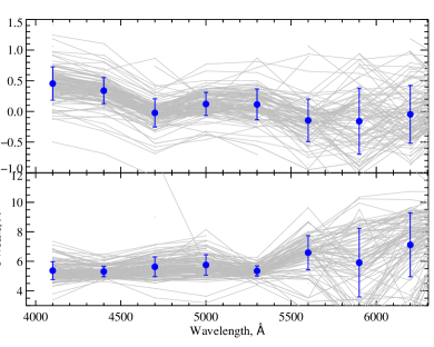
Figure 1: Relative LSF for the 127 NGSL stars in common with the ELODIE library. The panels show the shift in wavelength and the resolution (FWHM) as a fucntion of wavelength. The obtained LSFs for the individual stars are plotted in thin grey lines. The mean values and their standard deviations are plotted in blue.

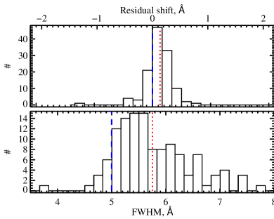
Figure 2: Histograms corresponding to the distributions of the wavelength shift and the resolution at $\sim$5000 Å for the 127 NGSL stars in common with ELODIE. The blue dashed vertical lines mark the zero velocity and the expected dispersion of 5 Å , while the red dotted lines are the mean residual shift and the mean FWHM (top and bottom respectively).

4.2 UVBlue theoretical grid

The UVBLue library (Rodríguez-Merino et al.  2005) covers the wavelength range from 87 nm to 470 nm at $R=50000$. Its parameter coverage reaches from T_eff = 3000 to 50 000 K, $log$g = 0.0 to 5.0 with steps of 0.5 dex, and [Fe/H]= -2.0 to 0.5 dex, computed at 7 nodes with a solar mix (Anders & Grevesse  1989). The final grid consists of 1770 models with local thermodynamic equilibrium (LTE). These were computed using the updated list of atomic transition given by Kurucz (1992), adding all diatomic molecular lines except TiO. However, the latest molecule transitions are only prominent in late-type stars with T_eff  bellow 4000 K, which in turn do not have significant UV flux. The microturbulent velocity was fixed ($\xi$ = 2 km s^-1, default for the Kurucz models). This value is expected to vary in the different spectroscopic classes from 1.5 to 10 km s^-1, but the effects are expected to be negligible at low resolution (as in the present case). We downloaded the $R=10000$ version available online, calibrated in air wavelength. We measured its intrinsic resolution using the solar spectrum from the BASS2000 database and found it to be consistent with the value given by the authors.

Each of the NGSL stars was fitted against a positive linear combination of UVBlue spectra according to Eq. 3.2. For each NGSL stellar spectrum the comparison was made with the eight UVBlue spectra whose parameters surround the values from Table LABEL:table:params (determined in Sect. 5). We determined the weights of the different UVBlue spectra from a fit over the whole wavelength range, and we used this combination to analyse the individual segments. This first fit of the whole spectral range was also used to clip the spikes. We performed the LSF analysis again in the 400 Å segments and we averaged the individual LSFs.

While fitting the LSF we noticed that the region between 2400 and 3000 Å is poorly matched by the theoretical spectra. This discrepancy was already pointed by the authors of UVBlue (Rodríguez-Merino et al.  2005), stating that the simulated FGK stars fail to reproduce important prominent metallic features as the Feii blend at 2400 Å, Fei/Sii blend at about 2500 Å, Mgii doublet at 2800 Å  Mgi line at 2852 Å and the Mg break at $\sim$ 2600 Å. We find that the match is also poor for the OBA and M spectral types (although the low flux of the M stars in the blue reduces the significance of the comparisons because of the S/N limitation). However, even though that many prominent features are misfitted, there is enough information in the other lines to constrain the LSF, but of course with a lower precision. Hence, the LSF determined in this region needs to be taken cum grano salis.

4.3 Munari et al. theoretical grid

To assess the LSF in the NIR part of the NGSL stars, we downloaded the 1 Å/px, scaled solar version of the Munari library ($\lambda\lambda=2500-10500$Å, Munari et al.  2005). The library of 51288 spectra was produced using Kurucz models covering the space of atmospheric parameters as follows: $3500\leq$ T_eff $\leq 47500$ K, $0.0\leq$ $log$g $\leq 5.0$, $-2.5\leq[M/H]\leq 0.5$, $[\alpha/Fe]=0.0,+0.4$, $\xi=1,2,4$ km s^-1, $0\leq V_{rot}\leq 500$ km s^-1. They used the updated list of atomic transition by Kurucz (1992), adding some molecular lines, including TiO for stars with T_eff $<5000$ K. The authors compared the colours and temperatures of their predictions to other synthetic libraries and real stars, noticing that their models fail to reproduce the very red colour observed in low-temperature stars.

We measured its intrinsic resolution using the solar spectrum from the BASS2000 database and found it to be FWHM = 2.1 Å throughout the full wavelength range. Again, the spectra are air-wavelength-calibrated. The Munari grid was generated at high resolution, then convolved with a Gaussian to lower resolution and finally rebinned to pixels of half the FWHM of this Gaussian. Since the rebinning also implies a convolution by a top-hat function of 1 pixel, the final broadening is slightly larger than the convolving Gaussian. We performed the LSF analyses over the full wavelength range in the same way as for UVBlue, following Eq. 3.2.

4.4 Corrected wavelength calibration and adopted LSF

The LSFs obtained with the four reference libraries are represented in Fig. 3. The results from these comparisons are fully consistent.

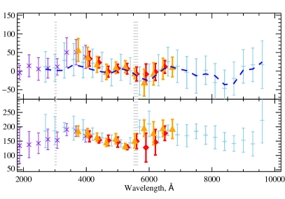
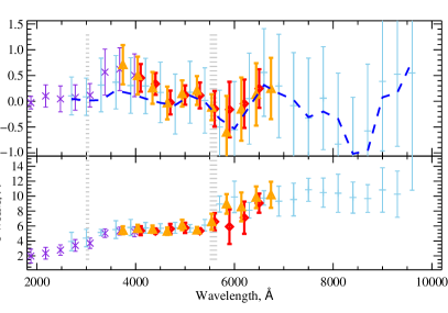
Figure 3: Global line-spread function of NGSL. The upper panels show the residual velocity and instrumental velocity dispersion in km s^-1. The bottom panels show the corresponding wavelength shift and resolution in Å. The LSFs obtained with the aid of the various reference libraries are overplotted with the symbols according to the legend in the first panel. The error bars represent the standard deviations from the distribution of the LSF obtained with the individual stars. The regions where the three segments of NGSL overlap are marked with grey horizontal lines. The blue dashed line shows the applied correction to the velocity shift. (MILES and ELODIE libraries have different starting points, therefore their results appear slightly shifted.)

The FWHM of the LSF is varying from 3 Å  at the UV end to 5 Å  at 5000 Å , and to 10 Å at the NIR end. It is roughly constant over each segment corresponding to the different gratings, and the discontinuities between the three gratings, at 3060 and 5650 Å , are clear.

The residual shifts for the UV and red gratings do not significantly depend on the wavelength and are small: 10 and 0 km s^-1. Our analysis reveals a defect of the wavelength calibration of the green segment (G430L grating). We used a simple linear relation to correct it: $\lambda_{cor}=\lambda-0.7(5650-\lambda)/(5650-3060)$, for $3060<\lambda<5650$ Å, where $\lambda$ is the original wavelength in Å and $\lambda_{cor}$ the corrected wavelength. This first-order correction of the dispersion relation is derived from the drift of the residual wavelength shift seen on Fig. 3. This correction can easily be applied to the wavelength array when the NGSL FITS files are read.

We averaged the four LSFs and restored the discontinuities, which were smoothed by our analysis in 400 Å segments by extrapolating the trend seen for each grating towards the overlap regions.

5 Atmospheric parameters

We determined the atmospheric parameters of the NGSL stars by fitting the spectra against a reference spectrum of given T_eff, $log$g and [Fe/H] . We compared the parameters with various previous studies to assess their reliability and precision.

5.1 Measurement of the parameters

We determined the atmospheric parameters of NGSL with ULySS as in Wu et al. (2011b), Prugniel et al. (2011), and Wu et al. (2011a). The fit is performed according to Eq. 4 over the wavelength range 3500 to 7500 Å (the wavelength range of the MILES stellar library). The spectra were logarithmically rebined to pixels corresponding to 100 km s^-1. We used the LSF derived in the previous section as described in Koleva et al. (2009). Because of the variation of the LSF throughout the library, the convolution by $G$ in Eq. 4 was maintained. To prevent that the model adapted to the mean NGSL resolution becomes broader than a given spectrum, we biased the injected LSF by 100 km s^-1 (i.e. we subtracted 100 km s^-1in quadrature from $\sigma_{ins}(\lambda)$). We used a 12^th degree multiplicative polynomial to absorb any continuum mismatches between the model and the observations (Sect. 3).

ULySS performs a local minimisation starting from a guess point in the parameter space. Thus, the solution may be trapped in a local minimum. To avoid this and reject local minima, we repeated the minimisation from multiple guesses, sampling the parameters spaces at the following nodes: T_eff in $[3500,4000,5600,7000,10000,18000,30000]$, [Fe/H] in $[-1.7,-0.3,0.5]$ and $log$g in $[1.8,3.8]$.

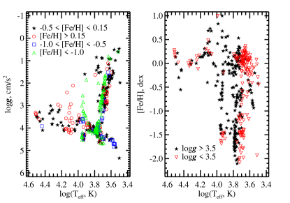
Figure 4: Resulting stellar parameter coverage for the 374 stars of the NGSL. The left panel shows their distribution in the T_eff - $log$g plane. These stars were separated into four different metallicity bins according to the legend. In the right panel we plot the dwarf and giant distribution in the T_eff -[Fe/H] plane.

Previous studies, in particular Wu et al. (2011b), have shown that while this method is highly reliable for FGK stars, special care has to be taken for OBA and M stars. There are various reasons for this lower reliability: First, the reference library is more scarcely populated in these regions of the parameters space; second, high-precisions measurements of the atmospheric parameters of these stars are not as abundant as for FGK stars; finally, the determination of the parameters of those stars is more complex for physical reasons. Therefore, we systematically checked our determinations against recent literature for OBA and M stars as well as for cases that we found in disagreement with other studies. For 30 stars (8 percent of the library) we adopted measurements from the literature. Our final list of parameters are given in Table LABEL:table:params. The distribution of the stars in T_eff - $log$g and T_eff - [Fe/H] planes is presented in Fig. 4.

5.2 Comparison with the literature

We compared our measured parameters with those from four previous studies by Heap & Lindler (2009), Wu et al. (2011b), Prugniel et al. (2011), and Soubiran et al. (2010).

Heap & Lindler (2009) derived preliminary, main atmospheric parameters of the NGSL (version 1). They derived T_eff and the metallicity by fitting the stellar spectra to models of Munari (Munari et al.  2005). The gravity was obtained from the star position on the HR diagram using the Hipparcos parallax for the distances. The comparison of their results with the Valenti & Fischer (2005) catalogue of cool stars shows some deviations for the $log$g, which are not unexpected because the atmospheric parameters are coupled, and deriving them separately may lead to biases.

The determination of the CFLIB and MILES parameters (Wu et al.  2011b; Prugniel et al.  2011) was performed as in the present paper. This method is highly reliable for intermediate spectral types, but it is not as accurate for the extremes of the HR diagram, as discussed in Section 5.1. There are, however, two main differences that may affect the comparison. On one hand, the presently analysed library has a much lower resolution than that of CFLIB (R$\sim$5000) and MILES (R$\sim$2000). The information from the weak lines accordingly is blended, which is particularly important when analysing earlier stellar types. On the other hand, the MILES interpolator, performs better than ELODIE (3.1 or 3.2) in some regions of the HR diagram (in particular for blue-horizontal branch stars, Prugniel et al. 2011). Hence, stars in this regions will possibly have a more precise determination of their atmospheric parameters.

Finally, the latest version of the PASTEL database (Soubiran et al.  2010) is a compilation of previously published stellar atmospheric parameters. It continues series of publications by Cayrel and collaborators (Cayrel de Strobel et al.  2001). Most of the measurements were made using high spectral resolution and high signal-to-noise data, though inhomogeneous. When there were multiple measurements of the same parameter of a given star available, we took the mean value.

The statistics of the comparisons was made without the outliers and it is presented in Table 5.2. The corresponding figures with the four comparison are given in Appendix LABEL:app:comparison.

Table 1: Comparison of the atmospheric parameters with other studies.

Comparison		N	$T_{{\rm eff}}$			log g (cm s-2)			[Fe/H] (dex)
			$\Delta$	$\sigma$	$\nabla$	$\Delta$	$\sigma$	$\nabla$	$\Delta$	$\sigma$	$\nabla$
NGSL	OBA	59	4	3	0.87	0.12	0.47	0.45	-0.10	0.60	0.56
	FGK	236	4	171	1.08	0.22	0.42	1.18	0.09	0.34	0.94
	M	6	-42	120	1.14	0.32	0.55	1.32	-0.35	0.40	-0.05
MILES	OBA	20	6	6	0.96	0.11	0.45	0.87	-0.02	0.19	0.99
	FGK	55	26	115	1.01	0.03	0.28	1.10	-0.00	0.11	1.01
	M	4	41	37	1.02	0.13	0.14	0.83	0.08	0.19	0.06
CFLIB	OBA	32	5	3	1.04	0.05	0.30	0.93	0.03	0.22	1.03
	FGK	80	43	111	1.00	-0.00	0.20	1.04	0.04	0.11	1.01
	M	5	37	23	0.98	0.46	0.69	0.24	0.17	0.29	1.00
PASTEL	OBA	57	7	6	1.06	0.06	0.43	0.65	-0.00	0.63	0.90
	FGK	176	69	196	1.00	0.04	0.42	1.09	0.05	0.19	1.03
	M	5	-73	246	0.51	-0.13	0.19	1.02	-0.26	0.33	0.60

The FGK stars agree well with the results of the other authors. The biases are within the errors of the individual parameters and are not significant.

The linear fit of the comparison has slopes ($\nabla$) close to unity in almost all cases. The dispersions from the comparisons are higher than in Prugniel et al. (2011), revealing a lower precision, which is probably caused by the lower spectral resolution.

The strongest discrepancy for the FGK spectral classes appears when comparing our $log$g values with that derived by Heap & Lindler (2009) from the same data (see Fig. LABEL:fig:compNGSL). Our gravities are up to one dex higher for the dwarfs. This is consistent with the bias found in Heap & Lindler (2009) by comparing to Valenti & Fischer (2005). The discretisation of the measurements of Heap & Lindler (2009) on the nodes of the model’s grid is also apparent in the figure. This is because the authors did not interpolate between the templates.

The automatic determination of the parameters is more difficult for OBA and M stars. At this low resolution only few lines are present for early-type stars, and the parameters are less constrained. In addition, the profiles of the lines are also affected by rotation (and inclination of the rotation axis on the line-of-sight) and some stars display emission lines. For the late types, on the other hand, the spectra are dominated by broad molecular features and the individual narrow band is lost because of the low resolution. Despite these difficulties, the comparison with previous studies revealed no trend or bias.

To summarise, our results are consistent with those of authors for all spectral types. The offsets in T_eff vary from 4 to 69 K in the FGK stars, depending on the comparison study with a dispersion of $\sim$ 150 K; in $log$g the offset found in comparison with Heap & Lindler (2009) is 0.22, while there is no offset with the other references, the typical dispersion is about 0.35 dex; the shift in metallicity is negligible and the dispersions are between 0.11 to 0.34 dex. For the OBA spectral types we find $\Delta(T_{eff},K)\sim 5$%, $0.05<\Delta(log$g$,cm/s^{2})<0.12$, with a dispersion $\sim 0.47$ and $-0.02<\Delta[Fe/H],dex<0.10$, varying between $0.2$ and $0.6$ dex. There are too few M stars in common between the different data sets to make any statistical analyses.

5.3 Error estimation

The errors returned by ULySS are computed from the covariance matrix. They underestimate the real precision because (i) the parameters are not fully independent (for example there is the well-known degeneracy between T_eff and $log$g), (ii) the fits are not perfect (there are some mismatches caused by non-solar abundances or particularities), and (iii) the errors in the data are not accurately known. Therefore, we first determined an upper limit to the internal error by forcing $\chi^{2}=1$, and we estimated the external error by rescaling the internal error as in Wu et al. (2011b).

To estimate the external errors we used the statistics of the comparison between our determination and Prugniel et al. (2011, see Sect. 5.2). We chose this reference for the comparison because it is homogeneous and reasonably accurate. The external errors were determined in Prugniel et al., therefore we subtracted them quadratically from the dispersion of the comparison and obtained an estimate of the mean external error. From this mean external error we derived the rescaling factor. For a given spectral type and stellar parameter, the rescaling factor is computed as

$$\xi=\frac{\sqrt{\sigma_{tot}^{2}-\bar{\sigma}_{mil}^{2}}}{\bar{\sigma}_{int}},$$ (5)

where $\sigma_{tot}$ is the residual dispersion from corresponding comparison in Table 5.2, $\bar{\sigma}_{mil}$ the external errors reported in Prugniel et al. (2011), and $\bar{\sigma_{int}}$ the mean internal error from the present fits. The final corrected error for each of the stars is $\sigma^{\prime}_{i}=\xi\times\sigma_{i}$.

The correction coefficients are about 2.5 for the FGK stars. For the early spectroscopic classes they vary from 2.5 (for metallicity) to 6.0 (for gravity). We do not have sufficiently high statistics to compute these coefficients for the M class. However, we consider that the external errors are roughly the same as for the OBA stars and as in Prugniel et al. (2011). Therefore, we used their coefficients to correct the errors of M stars. The median precision of the derived parameters is 42 K for T_eff, 0.24 dex in $log$g and 0.09 dex in [Fe/H] for the FGK class. For the OBA stars they are 4.5 percent, 0.44 dex and 0.18 dex, and for the M stars 29 K 0.50 dex and 0.48 dex for temperature, gravity, and metallicity, respectively. The precisions are lower than those obtained by Prugniel et al. (2011), probably because of the lower spectral resolution.

6 Galactic extinction

The Galactic extinction may be determined from photometry (e.g. Neckel & Klare  1980) or using a Galactic model (Chen et al.  1998; Hakkila et al.  1997). The first method requires (i) accurate photometry and (ii) a good knowledge of the intrinsic spectral energy distribution of the stars (i.e. a precise spectral classification). A wrong estimate of the metallicity will immediately translate into an error on the Galactic extinction. The second method requires knowledge of the direction and distance to the star and an adequate model of the Galaxy. For example the Chen et al. (1998) model is a simple geometric representation of the galaxy scaled to the “total” extinction provided by the Schlegel maps. Alternatively the Hakkila et al. (1997) model is calibrated on empirically measured extinctions in several directions in the galaxies. These models are generally acceptable in low-extinction regions (i.e. Galactic latitude $|b|>10^{\circ}$), but they are less reliable in high-extinction regions.

An alternative to these two methods is to directly measure the extinction on the NGSL spectra. The NGSL spectra were flux-calibrated with a precision of 2-3 percent (Heap & Lindler  2009). Therefore, $P_{n}$ mixes information about the uncertainty of the flux calibration and the Galactic extinction. Hence, we can assume to first approximation that $P_{n}$ (Eq. 4) derived in Sect. 5 corresponds to the extinction curve. We therefore fitted $P_{n}$ against the Galactic extinction law from Fitzpatrick (1999). The precision on the derived E(B-V) colour excess depends on the precision on (i) the flux calibration, (ii) the atmospheric parameters, and (iii) the best-fitted template. The precision of the ELODIE and MILES interpolators were discussed in Prugniel et al. (2011) and were found to be accurate to 1-2 percent.

The extinction law, $A(\lambda)/A_{V}$ (normalised to the V band) depends on the line-of-sight. It can be parameterised with $R_{V}=A_{V}/E(B-V)$ (the ratio between the extinction in the V and the B-V colour excess), which have a ‘mean’ value of 3.1, but it varies between 2.3 and 5.3 (Cardelli et al.  1989; Fitzpatrick  1999). The extinction is almost independent of $R_{V}$ in the red, but is strongly dependent on the wavelength in the blue and UV. Adopting the Fitzpatrick (1999) extinction law, we were able to fit simultaneously $A_{V}$ and $R_{V}$ over almost the full wavelength range by comparing the observed spectra to the Munari best fit. However, it is known that the SED of the theoretical spectra might not provide a good match to the empirical counterpart, particularly in the shortest wavelengths. For this reason, we preferred to compare the observations to the best-fitted interpolated MILES spectrum obtained in Sect. 5.

Fitting the extinction using MILES restricts the wavelength range to the optical domain, and therefore the correction of the whole spectrum requires extrapolations. The extrapolation towards the infrared should be safe because the extinction law is uniform in any line-of-sight (and the extinction is low), and the quality of the corrected spectrum will be essentially limited by the precision of the original flux calibration. However, the extrapolation towards the UV can be more hazardous because the determination of ${\rm R_{V}}$ will only rely on the blue end of the MILES spectra. Any error on the extinction law would be amplified in the UV. For this reason, we preferred here to adopt $R_{V}=3.1$ and we fitted only $A_{V}$ over the wavelength range 3500-7500 Å.

To test the reliability of these determinations of the extinction, we compared them with the predictions of the Chen et al. (1998) Galactic extinction model for the stars with parallaxes known from Hipparcos. This comparison is acceptable with a slope of 0.85. Our values of $A_{V}$ are listed in Table LABEL:table:params.

7 Conclusions

We have fully characterised the NGSL for its implementation in stellar population synthesis modelling. We used ULySS, a full spectrum fitting package. We found that the line-spread function of the stellar spectra of this library vary from 3 Å in the UV to 10 Å (FWHM) in the near IR. The instrumental velocity dispersion is virtually constant within the whole spectral range covered by the library, at $\sigma_{ins}\approx 130$ km s^-1. The wavelength calibration is accurate to 0.1 px (0.32 Å at 5000 Å). We measured the atmospheric parameters of the stars using the ULySS package and the MILES interpolator Prugniel et al. (2011). By comparing the results to previous studies we found that the precisions for the FGK stars are 42 K, 0.24 and 0.09 dex for T_eff, $log$g and [Fe/H], respectively. For the M stars, the corresponding mean errors are 29 K, 0.50 and 0.48 dex, and for the OBA 4.5 percent, 0.44 and 0.18 dex. Finally, we measured the Galactic extinction for each star by directly comparing the spectra to the interpolated MILES spectra.

The NGSL library is a major step towards the accurate modelling of stellar populations over a wide wavelength range. In the second paper of this series we make use of the NGSL and the results of this work to expand the spectral coverage of our stellar population models (Vazdekis et al.  2010).

Appendix A Atmospheric parameters

Here we list the adopted parameters of the 367 NGSL stars (Table LABEL:table:params), together with the extinction in $V$, the values of the S/N at 3 different wavelengths, roughly corresponding to the middle of the range from the blue, green, and red arm of the STIS spectrograph. There are 35 stars that SIMBAD recognises as spectroscopic binaries, they are marked with a star (*). Finally, in this table we give the references for the stars with parameters adopted from the literature.

1

Table 2: List of 367 stars in the NGSL. The columns are as follows: name; adopted atmospheric parameters and their errors (col 2 to 7); residual shifts in km s^-1; velocity dispersions in km s^-1, S/N at 3 different regions (col 10 - 12); extinction in $V$; reference for the atmospheric parameters. If not specified the measurements are from this paper.

Name	$T_{\rm eff}$	error	$log(g)$	error	[Fe/H]	error	cz	$\sigma$	S/N @
	(K)		($cm\,s^{-2}$)		(dex)		km s-1	km s-1	2800 Å	4000 Å	8000 Å	AV	Reference
bd+092860	5298	28	2.98	0.17	-1.99	0.06	-21	129	40	94	55	0.06
bd+112998	5480	30	3.00	0.24	-1.12	0.08	-3	182	99	251	349	0.11
bd+174708	6198	16	4.18	0.06	-1.56	0.05	-20	158	193	207	101	0.11
bd+292091	5615	17	3.68	0.08	-2.01	0.04	-5	145	116	139	72	0.06
bd+371458	5365	21	3.29	0.11	-2.01	0.05	-6	144	160	243	141	0.07
bd+381670	5535	22	4.11	0.10	-0.70	0.06	-21	162	88	219	290	0.07
bd+413306	5052	38	4.41	0.14	-0.53	0.08	-40	153	44	241	393	-0.00
bd+413931	5530	23	4.08	0.10	-1.48	0.06	31	145	81	129	75	0.12
bd+423607	5659	19	3.69	0.09	-2.11	0.04	17	141	127	146	73	-0.01
bd+442051	3664	11	4.70	0.05	-0.83	0.04	41	178	3	127	286	0.20
bd+511696	5746	16	4.39	0.06	-1.25	0.05	1	157	103	158	89	0.08
bd+592723	6035	15	4.00	0.06	-1.94	0.04	2	161	131	129	65	0.18
bd+660268	5240	29	3.45	0.17	-1.81	0.06	17	144	76	147	86	-0.12
bd+720094	6174	14	4.06	0.06	-1.76	0.04	26	170	170	169	83	0.11
bd+75d325	30086	1531	3.59	0.29	+0.22	0.11	-111	592	201	173	202	0.16
bd-122669*	6892	12	4.16	0.02	-1.47	0.03	-17	192	176	155	67	0.14	0
cd-259286	6336	16	4.11	0.03	-1.22	0.03	-31	139	67	117	132	0.29	0
cd-3018140	6151	17	4.01	0.07	-1.81	0.05	-4	154	162	167	78	0.02
cd-621346	5296	42	2.86	0.30	-1.44	0.10	7	147	69	173	246	0.22
cd-691618	29000	-	3.70	-	-0.30	-	-1	191	820	401	206	0.27	0,5
g019-013	4083	54	4.54	0.21	-0.58	0.19	-28	147	20	272	335	-0.32
g021-024	3995	19	4.49	0.07	-0.44	0.07	-30	147	11	144	213	0.06
g029-023	6143	19	4.09	0.07	-1.74	0.05	32	154	134	144	73	0.21
g114-26*	5966	12	4.14	0.05	-1.59	0.04	0	157	175	188	98	0.06
g115-58	6117	26	4.08	0.10	-1.65	0.07	2	148	47	56	26	0.15
g12-21	6021	16	4.19	0.06	-1.43	0.05	-7	159	120	144	74	0.10
g13-35	6015	18	3.99	0.07	-1.84	0.05	-20	170	186	189	96	0.05
g169-28	5849	18	4.21	0.07	-1.32	0.05	7	143	54	85	44	0.04
g17-25*	5271	23	4.44	0.09	-1.03	0.06	9	141	49	160	111	0.13
g18-39	6091	17	4.18	0.06	-1.47	0.05	23	161	115	132	69	0.10
g18-54*	6044	21	4.23	0.08	-1.51	0.06	12	160	94	111	59	0.20
g180-24	6042	13	4.13	0.05	-1.40	0.04	12	158	150	169	87	0.03
g187-40	5831	18	4.20	0.07	-1.49	0.05	24	143	89	121	64	0.07
g188-22	6038	14	4.16	0.06	-1.35	0.04	5	151	128	154	79	0.11
g188-30	5382	24	4.11	0.11	-1.37	0.06	9	146	32	82	48	-0.06
g192-43	6109	18	4.05	0.07	-1.69	0.05	-22	151	128	141	68	0.09
g194-22	5989	20	4.07	0.08	-1.69	0.05	-5	146	165	183	89	-0.06
g196-48*	5767	22	3.90	0.10	-1.75	0.06	-5	154	101	133	72	0.11
g20-15	6035	20	4.12	0.08	-1.66	0.06	-1	153	80	112	67	0.57
g202-65*	6656	20	4.25	0.08	-1.37	0.07	29	171	83	84	33	-0.10
g231-52	5414	25	3.86	0.13	-1.67	0.06	38	159	72	122	72	0.01
g234-28*	6066	17	4.13	0.07	-1.58	0.05	-6	159	81	95	47	0.14
g24-3	5962	21	4.06	0.09	-1.78	0.06	19	157	110	127	67	0.14
g243-62	4902	17	4.68	0.07	-1.13	0.05	-21	180	5	65	122	-0.05
g260-36	4962	30	4.45	0.10	+0.15	0.04	-18	153	7	70	134	0.04
g262-14*	5177	24	4.44	0.09	-0.68	0.06	2	147	10	73	119	0.14
g63-26	5996	28	3.92	0.12	-1.84	0.07	-11	153	46	55	25	0.15
g88-27	6071	17	4.12	0.07	-1.65	0.05	-3	162	104	115	58	0.07
gj825	3796	18	4.55	0.08	-0.62	0.07	98	148	27	234	573	0.10
gl109	3462	5	4.87	0.01	-0.20	0.20	102	142	0	53	144	0.11	0,7,9
gl15b	3630	12	4.71	0.02	-0.88	0.03	55	165	6	191	390	0.16	0
hd000319	8589	339	4.45	0.29	-0.54	0.29	5	178	790	581	535	-0.01
hd000358	12938	366	4.19	0.57	+0.42	0.19	0	236	904	572	470	0.05
hd000886	20700	822	3.81	0.33	-0.02	0.09	-1	160	1120	639	442	0.10
hd001461	5588	64	4.03	0.26	+0.08	0.10	-1	164	211	505	624	0.05
hd002665	5100	45	2.62	0.30	-1.88	0.09	37	141	141	375	278	0.35
hd002857	7607	12	3.78	0.09	-1.35	0.06	3	151	127	165	58	-0.12
hd003360	20703	984	3.83	0.41	-0.01	0.11	0	160	1455	606	452	0.13
hd003712	4778	63	2.06	0.33	+0.15	0.11	-16	153	97	205	412	0.11
hd004128	4848	62	2.25	0.36	+0.05	0.12	-8	149	224	276	512	0.03
hd004727*	14851	396	4.12	0.43	+0.14	0.17	7	210	1041	639	463	0.17
hd004813	6167	28	4.17	0.12	-0.18	0.06	1	144	342	467	494	0.12
hd005256	5170	36	3.59	0.22	-0.65	0.07	3	150	68	271	410	0.09
hd005395	4888	58	2.61	0.39	-0.42	0.12	-4	159	124	423	657	0.23
hd005544	4655	54	2.26	0.35	-0.04	0.10	-11	178	19	335	629	0.24
hd005916	4977	57	2.69	0.42	-0.78	0.13	1	160	97	450	642	0.23
hd006229	5174	32	2.58	0.24	-1.18	0.08	10	160	83	292	446	0.06
hd006734	4934	46	3.18	0.32	-0.58	0.09	-13	145	111	384	498	0.10
hd006755	5181	33	2.84	0.24	-1.52	0.07	32	144	162	386	266	0.17
hd008491	4790	50	2.60	0.31	+0.10	0.09	-14	155	120	314	535	0.20
hd008724	4976	39	2.43	0.30	-1.43	0.08	7	140	36	242	237	0.75
hd008890	6206	110	1.64	0.47	+0.19	0.20	-5	142	249	383	475	0.12
hd009051	5036	26	2.55	0.20	-1.51	0.06	11	143	58	209	158	0.23
hd010380	4191	41	1.88	0.40	-0.14	0.10	-38	141	44	244	532	0.24
hd010780	5400	76	4.54	0.19	+0.12	0.11	14	151	230	462	631	0.17
hd012533*	4402	44	1.84	0.28	+0.12	0.08	-31	138	103	184	576	0.55
hd013520*	4054	42	1.70	0.44	-0.13	0.12	-44	156	39	274	732	0.46
hd015089	8796	765	4.29	0.34	-0.94	0.63	32	128	701	523	438	0.01	0
hd016031	6104	14	4.07	0.06	-1.67	0.04	-14	164	177	180	91	0.02
hd017072	5352	53	2.83	0.40	-1.15	0.14	-1	151	306	526	632	0.01
hd017081*	13893	256	4.02	0.41	+0.21	0.13	-3	174	1101	606	474	0.15
hd017361	4700	44	2.67	0.30	+0.12	0.08	-17	154	103	298	519	0.24
hd017925	5286	81	4.69	0.19	+0.21	0.11	-5	153	163	366	522	0.29
hd018078	9791	289	3.43	0.36	+1.00	0.07	0	159	226	456	396	0.43	0
hd018769	8424	206	4.34	0.12	-0.02	0.15	34	128	673	564	516	0.05	0
hd018907	5059	76	3.56	0.48	-0.72	0.15	-11	150	165	528	698	0.08
hd019019	6033	32	4.26	0.12	-0.18	0.07	5	150	312	477	346	0.15
hd019308	5697	50	4.03	0.20	+0.06	0.08	6	149	154	453	289	0.13
hd019445	5805	18	3.79	0.08	-2.04	0.04	20	160	391	400	208	0.08
hd019656	4717	62	2.35	0.38	+0.05	0.11	-9	153	102	300	520	0.30
hd019787	4838	54	2.61	0.34	+0.13	0.09	-6	152	151	318	505	0.17
hd020039*	5206	37	3.66	0.21	-0.77	0.08	-2	150	65	253	387	0.13
hd020630	5694	58	4.39	0.18	+0.04	0.10	5	146	290	498	614	0.13
hd021742	5238	73	4.21	0.25	+0.32	0.09	2	150	63	358	588	0.08
hd022049	5146	74	4.68	0.19	+0.05	0.11	2	148	206	354	493	0.23
hd022484	5872	49	3.97	0.23	-0.23	0.11	-6	168	405	542	608	0.04
hd023439*	5198	41	4.38	0.17	-0.90	0.10	-5	162	77	358	522	0.08
hd025329	5020	40	4.42	0.19	-1.36	0.10	11	140	54	244	199	0.22
hd025893	5472	66	4.62	0.16	+0.26	0.09	0	145	114	378	335	0.27
hd025975	4921	67	3.29	0.40	+0.06	0.10	-8	145	92	350	530	0.15
hd026297	4827	62	2.01	0.44	-1.51	0.11	-9	137	30	328	355	0.84
hd026630*	5643	84	1.54	0.44	+0.10	0.18	0	142	391	341	564	0.84
hd027295	11013	337	4.06	0.50	+0.00	0.18	-2	212	1757	630	488	0.07
hd028946	5338	51	4.47	0.15	-0.08	0.09	-4	142	82	333	240	0.17
hd028978	8622	723	3.73	1.39	-0.75	0.52	-20	131	666	549	483	0.14
hd029391	7414	31	4.09	0.13	-0.02	0.08	-6	161	619	614	574	0.09
hd029574	4712	47	1.69	0.30	-1.52	0.10	-14	140	8	175	274	1.46
hd030614	32902	1917	3.31	0.23	+0.28	0.13	1	178	590	545	533	1.19
hd030834	4256	40	1.67	0.33	-0.24	0.09	-36	147	35	241	575	0.49
hd031219	6073	49	4.12	0.18	+0.17	0.08	6	139	146	407	476	0.14
hd031421	4541	37	2.43	0.28	-0.19	0.08	-39	151	105	268	516	0.26
hd033793	3722	28	4.71	0.05	-0.84	0.06	40	195	3	132	645	0.36	0
hd034078	31057	1696	3.54	0.25	-0.02	0.14	6	155	2571	678	572	2.11
hd034797	12273	355	4.23	0.50	+0.45	0.18	-9	232	910	624	490	-0.01
hd034816	26885	1880	3.60	0.29	-0.15	0.15	-7	188	1754	674	452	0.29
hd036702	4768	49	1.93	0.35	-1.78	0.09	0	135	14	205	249	1.14
hd036960	27000	-	4.10	-	-0.13	-	-9	176	1338	664	466	0.22	0,5,6
hd037202	21132	2024	3.24	0.41	+0.05	0.18	-55	232	1486	601	453	0.00
hd037216	5466	54	4.56	0.14	+0.05	0.09	10	141	96	358	246	0.17
hd037763	4555	72	3.17	0.49	+0.24	0.10	-16	156	72	345	687	0.04
hd037828	4726	76	2.04	0.60	-1.19	0.16	-14	168	38	380	671	0.62
hd038237	8279	471	4.32	0.63	-0.15	0.46	-11	179	667	615	529	0.09
hd038510	5846	29	3.96	0.16	-0.87	0.09	-21	164	220	412	488	0.07
hd039587*	5913	41	4.34	0.14	-0.10	0.08	8	144	298	444	507	0.15
hd039833	5871	49	4.39	0.15	+0.11	0.08	-3	147	142	422	256	0.15
hd040573	8795	367	3.60	0.54	-1.39	0.27	1	182	1027	612	492	-0.03
hd041357*	7838	52	3.88	0.08	+0.35	0.05	5	180	580	549	541	0.19	0
hd041661	6484	40	3.98	0.18	-0.03	0.08	0	165	287	488	257	0.14
hd041667	4838	84	2.31	0.65	-1.09	0.18	1	157	27	277	536	0.28
hd043042	6543	31	4.16	0.12	-0.02	0.07	-9	148	377	476	479	0.15
hd044007	5085	36	2.75	0.27	-1.50	0.08	-2	142	86	315	246	0.36
hd045282	5289	33	3.16	0.24	-1.46	0.08	-17	145	174	356	229	0.10
hd046703	6113	28	4.02	0.13	-1.30	0.09	6	141	77	226	134	0.30
hd047839	32130	1409	3.47	0.20	+0.13	0.10	6	227	1568	718	451	0.51
hd048279	31593	1806	3.51	0.23	+0.14	0.13	-7	176	1440	626	449	1.63
hd050420	7265	29	3.79	0.17	-0.00	0.08	-1	148	475	538	585	0.15
hd052089	22205	2741	3.35	0.45	+0.01	0.18	-2	182	989	831	406	-0.00
hd052973	5701	102	1.32	0.49	+0.12	0.20	8	155	238	473	668	0.48
hd055057	7234	33	3.87	0.18	+0.13	0.08	-9	162	553	566	578	0.04
hd055496	4935	85	2.33	0.65	-1.44	0.16	-8	141	51	243	207	0.36
hd057060	32508	1928	3.39	0.26	+0.24	0.14	58	247	2656	577	399	0.72
hd057061	32514	949	3.37	0.11	+0.18	0.07	9	222	2195	601	409	0.63
hd057727	4966	48	2.82	0.31	-0.17	0.09	-11	148	172	367	526	0.13
hd058343	17497	1268	3.29	0.55	+0.07	0.20	-17	223	708	630	562	0.55
hd058551	6246	23	4.21	0.11	-0.50	0.06	-4	176	446	575	613	0.09
hd059612	8306	686	1.60	0.37	-0.20	0.46	-12	157	520	556	566	0.16
hd060319	5907	17	4.03	0.09	-0.82	0.05	10	166	169	297	348	0.08
hd061064	6568	81	3.90	0.37	+0.06	0.16	-9	145	548	581	602	0.19
hd061603	3944	38	1.53	0.47	+0.18	0.14	-16	155	21	240	692	0.39
hd062412	4913	56	2.67	0.35	+0.04	0.10	-17	162	135	409	644	0.17
hd063077	5790	36	4.00	0.19	-0.79	0.10	-17	160	424	554	608	0.04
hd063700	5100	143	0.90	0.51	+0.14	0.24	-31	149	215	324	652	1.01
hd063791	5015	37	2.57	0.28	-1.47	0.08	5	145	64	314	270	0.49
hd064412	5688	25	4.05	0.12	-0.73	0.07	-11	161	136	307	382	0.06
hd065228	5992	118	1.43	0.52	+0.10	0.22	-8	152	382	507	667	0.27
hd065354	4146	45	1.34	0.33	+0.07	0.11	-15	153	15	242	709	0.79
hd065714	4908	105	2.21	0.57	+0.15	0.19	-39	156	104	398	619	0.10
hd067390	7142	15	3.96	0.08	-0.00	0.04	-10	157	155	237	234	0.18
hd068988	5755	47	4.00	0.20	+0.22	0.07	4	142	112	371	484	0.08
hd071160	4097	30	1.87	0.34	+0.07	0.08	-23	153	5	204	718	0.44
hd072184*	4643	71	2.84	0.47	+0.23	0.11	-35	158	58	358	665	0.11
hd072324	4858	86	2.32	0.50	+0.05	0.16	-32	163	75	384	597	0.15
hd072505	4596	87	2.81	0.59	+0.27	0.13	-32	159	36	343	660	0.24
hd072968	9645	1534	3.60	4.13	+0.83	0.43	39	228	639	574	510	-0.25
hd073710	4906	75	2.54	0.41	+0.23	0.12	-5	161	80	392	628	0.17
hd074088	4015	45	1.69	0.46	-0.26	0.13	-31	155	7	233	884	0.88
hd074721	8475	96	3.35	0.25	-1.47	0.11	1	153	420	417	295	0.05
hd076291	4609	60	2.81	0.44	-0.03	0.11	-22	155	61	360	659	0.21
hd076932	5894	30	4.07	0.15	-0.90	0.09	-8	163	444	567	625	0.08
hd078316*	12279	613	2.94	0.57	+0.22	0.18	-11	188	883	622	481	0.03
hd078362*	7343	100	3.86	0.43	+0.57	0.15	5	141	461	539	568	0.19
hd078479	4580	95	2.87	0.64	+0.33	0.13	-13	160	19	329	665	0.28
hd079158	12737	717	3.09	0.68	+0.49	0.18	-19	160	872	625	480	-0.07
hd079349	3884	19	1.79	0.26	+0.04	0.09	-12	153	2	147	681	0.34
hd079469	8691	234	3.23	0.34	-1.48	0.18	4	169	913	572	481	-0.12
hd080607	5389	45	3.99	0.18	+0.35	0.06	2	152	43	221	341	0.04
hd081797	4186	39	1.73	0.35	+0.07	0.09	-20	142	53	180	650	0.38
hd082395	4823	74	2.79	0.47	+0.04	0.13	-16	146	107	327	544	0.32
hd082734	4935	81	2.50	0.43	+0.26	0.13	-7	164	154	395	637	0.16
hd083212	4763	58	1.79	0.39	-1.39	0.11	-10	138	21	228	232	0.44
hd085380	5957	48	3.98	0.22	-0.06	0.09	3	145	289	466	633	0.11
hd086322	4804	46	2.53	0.30	-0.05	0.09	-4	151	44	336	424	0.22
hd086986	8031	84	3.57	0.45	-1.47	0.19	3	160	482	547	428	0.13
hd087140	5145	20	2.75	0.14	-1.73	0.04	15	145	97	218	151	0.09
hd087737	11522	640	2.11	0.37	+0.19	0.16	-16	142	1190	628	486	0.03
hd090862	4129	36	1.70	0.36	-0.39	0.09	-55	154	3	157	599	0.52
hd091316	21576	668	3.01	0.05	-0.06	0.06	4	181	959	621	476	0.07	0
hd093329	8127	84	3.45	0.41	-1.45	0.17	-22	160	351	390	292	0.05
hd093813	4456	41	2.36	0.33	-0.10	0.09	-25	144	114	247	527	0.35
hd094028	5982	17	4.09	0.07	-1.54	0.05	-5	167	316	365	191	0.06
hd095241*	5778	37	3.78	0.21	-0.47	0.09	0	151	333	459	509	0.09
hd095418	8734	542	3.68	1.12	-0.76	0.32	-1	141	723	441	425	-0.03
hd095735	3574	12	4.73	0.07	-0.93	0.05	8	157	9	237	535	-0.02
hd095849	4526	48	2.38	0.32	+0.21	0.08	-5	152	33	329	661	0.19
hd096446	20086	530	3.59	0.08	+0.06	0.04	-7	202	915	643	486	0.23	0
hd097633	8790	351	3.59	0.89	-0.64	0.18	-11	151	805	582	481	-0.04
hd099648	4970	75	2.25	0.43	-0.01	0.15	-10	144	153	403	618	0.28
hd101013*	5043	332	2.93	2.06	+0.12	0.54	2	172	126	384	587	0.71
hd101107	7036	16	4.09	0.08	-0.02	0.04	-7	208	781	538	562	0.10
hd102212	3738	6	1.55	0.10	-0.41	0.05	-9	150	36	218	539	0.12	12
hd102780	3835	22	1.64	0.31	-0.20	0.12	-24	156	3	162	751	0.53
hd103036	4688	80	1.64	0.53	-1.40	0.17	6	145	21	225	273	0.85
hd105452	7049	19	4.11	0.10	-0.21	0.06	-9	181	588	578	571	0.09
hd105546	5242	31	2.73	0.22	-1.46	0.07	11	138	105	264	173	0.05
hd105740	4771	34	2.77	0.26	-0.69	0.07	-21	180	26	263	520	0.18
hd106304	8675	205	2.85	0.18	-1.63	0.11	-6	160	362	358	246	0.04
hd106516*	6236	26	4.20	0.12	-0.70	0.08	2	167	500	581	607	0.07
hd107582*	5540	36	4.13	0.16	-0.72	0.09	10	152	157	393	506	0.06
hd108945	8906	1668	4.19	1.54	-1.48	1.36	37	128	613	568	498	0.03
hd109387	16906	1478	3.19	0.62	-0.12	0.31	-47	321	1965	526	417	0.29
hd109995	8427	174	3.41	0.45	-1.52	0.18	22	162	661	602	502	0.09
hd110073	13000	-	3.90	-	-0.40	0.30	-10	175	975	620	463	0.27	0,3,5
hd110885	5528	29	3.09	0.22	-1.21	0.08	16	147	100	214	130	0.11
hd111464	4314	43	2.17	0.40	-0.03	0.09	-30	162	13	284	713	0.64
hd111515	5373	48	4.23	0.19	-0.59	0.11	1	154	111	379	535	0.07
hd111721	5120	37	2.90	0.28	-1.27	0.08	9	141	102	333	248	0.22
hd111786	7549	45	4.17	0.21	-1.06	0.21	3	190	774	600	564	0.09
hd112413	11658	471	3.78	1.19	+0.68	0.17	-1	163	1036	541	452	-0.08
hd113002	5152	37	2.53	0.28	-1.08	0.09	0	153	68	271	414	0.04
hd113092	4319	38	1.53	0.33	-0.70	0.09	-24	152	35	318	701	0.24
hd114330	9671	289	3.57	0.82	-0.24	0.12	-5	134	641	429	373	0.24
hd114710	5973	49	4.23	0.18	-0.04	0.09	2	147	378	532	593	0.11
hd115617	5506	57	4.30	0.18	-0.03	0.10	0	144	228	410	500	0.13
hd117880	9000	-	3.01	0.03	-1.62	0.03	-14	143	344	354	247	0.23	0,15,4
hd118055	4717	38	1.74	0.25	-1.57	0.07	0	138	8	148	198	1.13
hd119971	4233	42	1.67	0.43	-0.61	0.10	-49	144	24	309	696	0.28
hd121146	4454	47	2.92	0.41	+0.03	0.09	-30	158	26	280	569	0.20
hd122064	4490	68	4.30	0.37	+0.09	0.11	-1	147	57	314	527	-0.22
hd122956	4932	61	2.33	0.47	-1.47	0.12	-11	148	61	376	376	0.62
hd123657	3261	43	0.59	0.38	-0.02	0.19	-15	165	39	246	987	0.28	13
hd124186	4458	57	2.79	0.44	+0.31	0.08	-25	154	25	315	642	0.21
hd124425*	6355	39	4.01	0.18	-0.10	0.09	-1	148	521	555	578	0.11
hd124547*	4165	48	1.73	0.45	-0.19	0.11	-47	142	222	244	574	0.19
hd126327	3100	0	1.98	6.27	-0.45	3.47	22	175	7	313	424	0.27
hd126511	5402	38	4.16	0.13	+0.17	0.06	1	160	66	272	193	0.07
hd126614	5453	59	3.87	0.25	+0.53	0.07	-5	158	42	245	392	0.05
hd126661	7809	91	3.83	0.35	+0.36	0.13	-1	169	613	560	547	0.11
hd128000	3954	33	1.75	0.41	+0.09	0.12	-21	154	21	256	744	0.38
hd128279	5279	22	3.07	0.13	-2.08	0.04	16	150	219	356	229	0.22
hd128801	8811	283	2.55	0.16	-1.69	0.11	16	185	492	424	269	-0.09
hd128987	5638	69	4.63	0.16	+0.09	0.11	0	147	132	424	306	0.22
hd131873	4077	28	1.70	0.29	-0.10	0.08	-15	151	86	179	672	0.39
hd132345	4484	67	2.58	0.47	+0.37	0.09	-23	165	31	316	634	0.16
hd132475	5721	20	3.79	0.10	-1.61	0.05	-13	150	220	296	170	0.10
hd134113*	5668	24	3.85	0.14	-0.82	0.07	4	165	171	384	465	0.06
hd134439	5357	35	4.68	0.10	-1.11	0.08	38	134	51	180	121	-0.04
hd134440	5094	36	4.70	0.12	-1.09	0.09	30	154	31	158	128	0.20
hd136726	4235	37	2.00	0.35	+0.02	0.08	-43	147	34	239	551	0.31
hd137759	4525	46	2.52	0.34	+0.13	0.08	-20	147	120	270	388	-0.27
hd137909	8620	499	3.96	1.18	+1.00	0.00	-9	154	627	495	483	0.23
hd138716	4767	54	3.05	0.36	-0.01	0.09	-15	150	123	312	520	0.15
hd138749	16150	346	3.75	0.38	+0.13	0.11	4	220	1063	605	439	0.23
hd140232	8381	238	4.27	0.17	+0.26	0.15	6	147	695	572	531	0.18	0
hd141795	8516	184	4.48	0.09	-0.17	0.14	41	128	753	552	518	0.01	0
hd141851	8524	383	4.27	0.39	-0.47	0.30	4	222	771	572	521	0.10
hd142091	4769	54	2.97	0.36	+0.07	0.09	-4	149	135	328	516	0.07
hd142703	7235	26	4.12	0.15	-1.20	0.13	-3	185	722	590	580	0.06
hd142860	6275	29	4.12	0.13	-0.26	0.07	7	164	383	490	476	0.11
hd142926	12831	782	3.33	1.03	+0.27	0.24	-8	235	806	619	484	0.19
hd143107	4460	44	2.20	0.34	-0.11	0.09	-16	137	75	269	508	0.29
hd143459	10298	277	3.85	0.50	-0.47	0.12	2	182	940	588	514	0.39
hd145328	4783	59	2.96	0.40	-0.00	0.10	-6	157	161	394	643	0.14
hd146051	3783	20	1.45	0.19	-0.03	0.06	-10	146	71	230	572	0.28	13
hd146233	5696	57	4.20	0.21	-0.06	0.10	1	148	250	433	486	0.11
hd147394	14906	332	4.06	0.39	+0.14	0.15	-5	201	1154	636	469	0.12
hd147550	9830	279	3.70	0.66	-0.38	0.11	-1	153	960	599	515	0.42
hd148293	4695	62	2.37	0.38	+0.20	0.11	-8	158	79	361	647	0.14
hd148513	4147	41	2.13	0.48	+0.21	0.09	-18	152	21	263	638	0.50
hd149161	3951	25	1.79	0.28	-0.18	0.09	-13	153	24	214	599	0.36
hd149382	27535	1985	3.92	0.76	-0.55	0.16	-36	522	1491	500	218	0.44
hd155763	14035	332	3.57	0.44	+0.22	0.11	-3	176	1002	605	448	0.19
hd156283	4274	45	1.78	0.35	+0.10	0.09	-32	151	27	259	796	0.50
hd157244	4479	89	1.37	0.37	+0.23	0.14	-35	153	182	270	634	0.86
hd159181	5325	87	1.51	0.47	-0.02	0.20	-15	159	362	431	553	0.44
hd160346*	4808	65	4.53	0.22	+0.03	0.10	-15	154	84	336	512	0.05
hd160762	17789	604	3.87	0.46	+0.00	0.13	0	169	1018	635	468	0.19
hd160922*	6595	28	4.19	0.11	-0.03	0.06	-1	160	494	564	595	0.12
hd161770	5782	20	3.95	0.09	-1.60	0.05	5	169	98	163	108	0.56
hd163346	6910	133	4.02	0.55	+0.23	0.23	90	250	418	430	387	0.69
hd163641	11953	263	4.06	0.44	+0.19	0.15	2	188	1283	609	519	0.41
hd163810	5818	15	4.35	0.06	-1.20	0.04	-11	148	102	156	86	0.11
hd164058	3985	32	1.69	0.38	+0.11	0.11	-18	164	133	237	664	0.34
hd164257	9792	691	3.70	2.11	+0.41	0.30	-10	178	720	610	526	0.38
hd164353	17574	662	2.96	0.23	+0.15	0.11	-9	155	3635	608	506	0.48
hd164402*	29405	374	3.30	0.02	+0.02	0.03	-8	158	5697	707	522	0.93	0
hd164967	9001	548	4.34	0.36	-1.32	0.43	36	128	794	616	523	0.14
hd165195	4766	59	1.89	0.40	-1.98	0.09	7	134	20	303	428	1.54
hd165341*	5365	62	4.49	0.16	+0.19	0.09	-2	141	185	339	462	0.24
hd166208*	4953	75	2.19	0.46	-0.06	0.16	-13	160	292	419	595	-0.04
hd166229	4577	67	2.82	0.47	+0.23	0.10	-34	177	61	349	644	0.10
hd166283	8574	616	4.55	0.53	-0.41	0.57	29	128	459	571	473	0.21
hd166991	8977	1010	4.40	0.55	-1.39	0.79	27	147	844	606	511	0.02
hd167006	3535	24	0.99	0.29	-0.08	0.10	41	148	28	188	735	0.38	13
hd167105	8637	143	3.25	0.24	-1.52	0.10	15	143	325	356	235	0.07
hd167278	6563	18	4.14	0.08	-0.21	0.04	1	149	245	363	173	0.12
hd167946	9300	502	3.74	0.87	-0.77	0.20	0	163	1024	616	494	0.27
hd169191	4426	41	2.22	0.33	-0.12	0.09	-26	143	44	272	554	0.35
hd170737*	5042	44	3.25	0.31	-0.87	0.09	11	154	69	346	564	0.13
hd170756	5903	106	3.79	0.61	-1.17	0.32	23	140	107	461	656	0.74
hd170973	12046	925	3.56	1.74	+0.73	0.28	-6	140	816	587	500	0.18
hd172230	7772	102	3.76	0.44	+0.55	0.14	0	188	458	587	528	0.12
hd172506	7078	20	4.00	0.10	-0.15	0.06	-5	141	304	427	181	0.06
hd173158	5164	121	0.87	0.43	+0.04	0.20	-1	154	10	206	857	2.28
hd173819	3650	102	0.51	1.38	-0.11	0.88	5	179	17	212	672	-0.79
hd174240	8879	340	3.61	0.88	-0.63	0.16	-7	166	809	583	514	0.12
hd174959	14321	348	4.05	0.48	+0.18	0.17	3	195	1054	636	485	0.27
hd174966	7874	57	4.09	0.16	+0.03	0.10	-9	152	430	575	505	0.32
hd175156	16361	556	3.04	0.25	+0.17	0.10	1	139	465	523	572	1.01
hd175305	5118	42	2.75	0.31	-1.43	0.09	15	139	151	426	323	0.05
hd175545	4526	53	2.95	0.40	+0.12	0.09	-24	161	16	337	674	0.26
hd175640	12067	326	4.07	0.55	+0.22	0.18	0	176	829	608	496	0.29
hd175674	4421	114	2.44	0.90	+0.21	0.20	-27	161	18	294	722	0.57
hd175805	6273	47	3.98	0.21	+0.15	0.08	1	144	195	445	239	0.19
hd175865	3181	52	0.47	0.47	-0.29	0.33	-9	156	74	224	800	0.14	13
hd176232	8659	308	4.47	0.33	+0.55	0.17	0	153	585	552	515	0.17
hd176437	12715	367	3.68	0.67	+0.17	0.15	0	128	844	534	496	0.38
hd181720	5659	42	3.88	0.23	-0.65	0.10	9	152	191	481	598	0.06
hd183324	8939	304	4.53	0.23	-1.30	0.50	13	312	764	550	474	-0.26
hd183915	4091	129	0.91	1.07	-1.17	0.42	-1	145	23	309	735	-0.41
hd184266	5700	-	2.00	-	-1.65	-	35	147	239	452	270	0.41	0,14,15,16
hd185144	5283	72	4.51	0.20	-0.11	0.12	7	151	204	384	515	0.17
hd185351	4921	56	2.95	0.36	+0.01	0.09	-2	143	163	356	519	0.09
hd187111	4764	59	1.93	0.42	-1.44	0.11	0	142	18	269	339	1.07
hd187879	20420	1274	3.18	0.28	-0.02	0.14	-12	197	688	608	517	0.40
hd188262	5749	108	2.80	0.68	+0.15	0.20	4	149	369	375	285	0.62
hd190073	10900	546	4.13	0.66	-0.02	0.26	181	273	434	610	463	0.60
hd190360	5427	74	3.93	0.31	+0.20	0.10	-4	180	282	485	610	0.05
hd190404	4982	55	4.49	0.20	-0.62	0.13	-10	146	83	395	332	0.04
hd191026	5133	69	3.77	0.33	+0.04	0.10	-4	167	200	370	518	0.19
hd191277	4462	50	2.89	0.41	+0.16	0.08	-26	156	45	328	667	0.12
hd193281	8623	345	4.30	0.33	-0.68	0.28	-4	192	755	544	489	0.03
hd193495*	5458	125	2.55	0.65	+0.13	0.21	10	161	868	417	669	0.18
hd194093	6000	-	0.85	0.10	+0.15	0.09	11	155	354	473	442	0.72	0,8,10,11,12
hd194453	10342	294	3.69	0.79	-0.06	0.14	-6	180	838	591	504	0.23
hd195434	4858	22	4.40	0.09	-0.57	0.05	-46	177	40	184	348	0.09
hd196218	6207	24	4.11	0.11	-0.19	0.05	0	150	279	487	271	0.10
hd196426	12951	187	4.10	0.27	+0.22	0.10	0	204	785	517	413	0.16
hd196662	15439	90	3.90	0.06	+0.14	0.03	-9	179	596	474	363	0.29	0
hd196725	4260	61	1.18	0.32	+0.06	0.13	-26	160	38	256	744	0.66
hd196892	6028	22	4.17	0.10	-0.99	0.07	6	165	257	412	469	0.06
hd197177	4955	74	2.07	0.40	+0.02	0.14	0	162	120	373	619	0.31
hd198809	5075	43	2.54	0.28	-0.27	0.09	5	154	264	381	514	0.02
hd200081	5526	71	3.25	0.43	+0.02	0.12	9	147	159	322	241	0.40
hd200905	3997	39	0.92	0.26	+0.12	0.12	-42	148	271	193	600	0.54
hd201091	4167	56	4.54	0.28	-0.35	0.20	20	156	75	330	695	-0.12
hd201377	8415	542	4.32	0.62	-0.23	0.46	0	166	731	589	518	0.12
hd201601	8574	406	4.47	0.51	+0.68	0.22	9	163	759	591	511	0.26
hd203638	4647	92	2.81	0.59	+0.27	0.14	-23	166	55	353	654	0.26
hd204041	8617	295	4.49	0.25	-0.61	0.28	6	174	828	578	545	0.04
hd204155	5704	28	3.89	0.16	-0.70	0.07	5	172	151	349	430	0.03
hd204543	4874	50	1.99	0.34	-1.78	0.08	15	134	40	256	224	0.34
hd204867	5715	100	1.22	0.46	+0.10	0.19	-4	144	219	385	489	0.38
hd205202	6496	22	4.07	0.10	-0.51	0.06	0	170	286	456	473	0.07
hd205811	9069	753	4.42	0.42	-1.30	0.61	23	146	1203	683	484	-0.23
hd206778	4240	47	0.93	0.21	+0.08	0.10	-10	145	226	142	558	0.67
hd210745	4337	81	1.12	0.33	+0.17	0.14	-37	157	157	246	632	0.89
hd210807	5023	54	2.31	0.33	-0.16	0.11	1	143	189	350	516	0.21
hd212516	3709	11	1.54	0.20	-0.24	0.09	-7	150	1	118	677	0.51
hd212593	13642	251	2.42	0.06	+0.30	0.04	-6	158	1228	628	526	0.50	0
hd215665	4933	78	2.25	0.42	+0.12	0.14	7	152	145	313	510	0.41
hd217107	5495	63	3.99	0.25	+0.30	0.08	-8	165	190	480	615	0.03
hd217357	3894	25	4.48	0.10	-0.47	0.10	-16	149	20	245	703	0.13
hd221377	6399	28	4.08	0.13	-0.66	0.08	-12	176	439	588	614	0.09
hd222404*	4734	56	3.10	0.37	+0.13	0.08	-14	159	334	356	565	0.08
hd224801	12704	568	4.11	0.94	+0.69	0.21	-4	188	1191	604	490	0.13
hd224926	14120	317	4.06	0.51	+0.31	0.16	-7	192	915	626	481	0.15
hd232078	4295	48	0.82	0.27	-1.08	0.11	-11	146	1	106	333	2.21
hd284248	6098	16	4.12	0.06	-1.60	0.05	-27	157	228	235	116	0.05
hd345957	5883	17	4.02	0.07	-1.45	0.05	11	146	201	257	143	0.08
hr0753	4529	74	4.40	0.38	-0.21	0.15	-13	149	67	300	446	-0.45
hr8086	3894	27	4.54	0.09	-0.56	0.09	-15	148	39	239	563	0.03
lhs10	3167	12	5.34	0.03	-0.42	0.10	-36	128	4	14	235	2.26	0
lhs482	3707	17	4.83	0.07	-0.78	0.07	-53	162	1	27	154	0.38
mmj6476	7648	22	3.96	0.09	+0.28	0.04	-11	156	66	106	98	0.27
mmj6490	8947	211	4.36	0.15	-1.37	0.21	14	135	130	142	104	0.02
vbnvul	7944	44	1.85	0.01	-1.58	0.04	52	163	32	102	70	1.67	0
vgkcom	3254	16	0.60	0.12	-1.93	-	-10	149	11	229	926	0.27	0,1
viwcom	3303	28	0.61	0.46	+0.08	0.34	-18	146	6	166	516	0.27

Table 2: continued.

Appendix B Comparison with other libraries

Here we plot the comparisons with the literature discussed in Sect. 5.2. For each of the reference libraries we plot the different spectroscopic classes in different panels. We omit the M class because there are too few (14) cold stars in NGSL. We provide the usual ‘our’ vs. ‘literature’ value plots, but we also investigate how the residuals of this comparison depend on the different parameters.