Computation of generalized inverses
using $Php/MySql$ environment

Abstract

The main aim of this paper is to develop a client/server based model for computing the weighted Moore-Penrose inverse using the partitioning method as well as for storage of generated results. The web application is developed in the $PHP$/$MySQL$ environment. The source code is open and free for testing by using a Web browser. Influence of different matrix representations and storage systems on the computational time is investigated. The CPU time for searching the previously stored pseudo-inverses is compared with the CPU time spent for new computation of the same inverses.

AMS Subj. Class.: 15A09, 68P15, 68N15.

Key words: PHP script, MySQL database, Weighted Moore-Penrose inverse, Matrix storage formats.

1 Introduction

Since the mid-1990s, there has been a surge of interest among the academics and practitioners in an open source software ($OSS$). There are many successful projects in $OSS$ community, primarily the $Mozilla$ web browser, the $Linux$ operating system, the $Apache$ web server, and to a lesser extent, $PHP$ [12] and the $Perl$ programming languages, as well as the $MySQL$ database. $OSS$ has drawn the attention of users and developers because of its economic benefits [10].

$PHP$ is an open source software, and it is free for downloading and use. Main characteristics of $PHP$ are described in [12].

$MySQL$ has become the world’s most popular open source database system because of its consistent fast performance, high reliability and ease of usage. Besides the fact that it is free, $MySQL$ offers a wide range of possibilities [5, 27].

$SQL$ is the standard language used for querying and analysis of data in a relational $DBMS$ [4]. Unfortunately, $SQL$ has no vector and matrix computations. Interesting code for matrix $SQL$ operations can be found in [16]. The $SQL$ constructions and the $SQL$ primitives for data mining are proposed in [1]. However, these constructions do not offer adequate and flexible tools for matrix manipulation. A graphical $SQL$ query generator and query operators with embedded matrix objects are disclosed in [3].

Implementation of some vector and matrix operations based on programming User-Defined Functions ($UDFs$) is studied in [15]. $UDFs$ represent a $C$ programming interface that allows the definition of scalar and aggregate functions that can be used in $SQL$. $UDFs$ have several advantages and limitations. An $UDF$ allows fast evaluation of arithmetic expressions, memory manipulation, using multidimensional arrays and exploiting all $C$ language control statements.

The organization of the paper is as follows. Motivation of the paper is described in the second section. In the third section, we describe application details. In the fourth section, we develop data storage and computing system, which manipulate with different types of matrices, based on the $PHP/MySQL$ environment. Functions and procedures are hardwired to a common matrix table. Influence of different matrix representations in conjunction with storage systems to performances of the implemented software is considered through numerical experiments. All test matrices and the results can be stored in files and the database on the server-side. A few illustrative examples and comparative studies are presented in the last section.

2 Preliminaries and motivation

Some mathematical formulations and motivation are involved in this section. Let $\mathbb{C}$ be the set of complex numbers, $\mathbb{C}^{m\times n}$ be the set of $m\times n$ complex matrices, and ${\mathbb{C}}^{m\times n}_{r}\!=\!\{X\in{\mathbb{C}}^{m\times n}\,:\,\,\,\mathrm{rank}({X})\!=\!r\}$. For any matrix $A\in\mathbb{C}^{m\times n}$ and positive definite matrices $M$ and $N$ of the orders $m$ and $n$ respectively, consider the following equations in $X$, where $*$ denotes conjugate and transpose:

$$\begin{array}[]{ll}(1)\qquad\ AXA=A&(2)\qquad XAX\!=\!X\\ (3M)\quad(MAX)^{*}=MAX&(4N)\quad(NXA)^{*}\!=\!NXA.\end{array}$$

The matrix $X$ satisfying (1), (2), (3M) and (4N) is called the weighted Moore-Penrose inverse of $A$, and it is denoted by $X=A_{MN}^{\dagger}$. In the particular case $M=I_{m}$ and $N=I_{n}$, the matrix $X=A_{MN}^{\dagger}$ comes to the Moore-Penrose inverse of $A$, and it is denoted by $X=A^{\dagger}$.

The Greville’s partitioning method for numerical computation of generalized inverses is introduced in [6]. The following computational experience is delivered in [11]: ”when applied to a square, fully populated, non-symmetric case, with independent columns, the Greville’s algorithm found that the approach can be up to eight times faster than the conventional approach of using the SVD; rectangular cases are shown to yield similar levels of a speed increase”. Due to its computational dominance, this method has been extensively applied in many mathematical areas, such as statistical inference, filtering theory, linear estimation theory, optimization and more recently analytical dynamics [25] (see also [9]). An application of the partitioning method in a direct approach for computing the gradient of the pseudo-inverse is presented in [11]. It has also found wide applications in the database and the neural network computation [13]. In the paper [7], the sequential determination of the Moore-Penrose generalized inverse matrix by dynamic programming is applied to the diagnostic classification of electromyography signals.

The Greville’s partitioning algorithm is extended in many papers. Wang in [26] generalizes Greville’s method to the weighted Moore-Penrose inverse. The algorithm for computing the Moore-Penrose inverse of one-variable polynomial and/or rational matrices, based on the Greville’s partitioning algorithm, is established in [19]. An extension of the results from [19] to the set of two-variable rational and polynomial matrices is introduced in the paper [18]. In the paper [22] we extended the Wang’s partitioning method from [26] to the set of one-variable rational and polynomial matrices. An efficient implementation of the algorithm introduced in [22] is established in [17]. An implementation of the algorithm introduced in [21] for computing generalized inverses is based on the $LU$ factorization of the matrix product.

For the sake of completeness, we restate the algorithm introduced in [26], applicable to rational and constant matrices. The algorithm is quite appropriate for computation of the weighted Moore-Penrose inverse as well as the Moore-Penrose inverse and regular inverse.

• 0:  Let $A\in\mathbb{R}^{m\times n}$, $M$ and $N$ be p.d. matrices of the order $m$ and $n$ respectively.

  1:  $A_{1}=a_{1}.$

  2:  if $a_{1}=0,$ then

  3:     $X_{1}=(a_{1}^{*}Ma_{1})^{-1}a_{1}^{*}M;$

  4:  else

  5:     $X_{1}=0.$

  6:  end if

  7:  for $k=2$ to $n$ do

  8:     $d_{k}\!=\!X_{k-1}a_{k},$ $c_{k}=a_{k}-A_{k-1}d_{k},$

  9:     if $c_{k}\neq 0,$ then

  10:        $b_{k}^{*}=(c_{k}^{*}Mc_{k})^{-1}c_{k}^{*}M,\ {\bf goto}\ Step\ \ref{sest},$

  11:     else

  12:        $\delta_{k}=n_{kk}+d_{k}^{*}N_{k-1}d_{k}-(d_{k}^{*}l_{k}+l_{k}^{*}d_{k})-l_{k}^{*}(I-X_{k-1}A_{k-1})N_{k-1}^{-1}l_{k},$

  13:        $b_{k}^{*}=\delta_{k}^{-1}(d_{k}^{*}N_{k-1}-l_{k}^{*})X_{k-1},$

  14:     end if

  15:     $X_{k}=\left[\begin{array}[]{cc}X_{k-1}-(d_{k}+(I-X_{k-1}A_{k-1})N_{k-1}^{-1}l_{k})b_{k}^{*}\\ b_{k}^{*}\end{array}\right].$

  16:  end for

  17:  return $A_{MN}^{\dagger}=X_{n}.$

   

Comparison of searching in large databases with recomputation in recursive algorithms is one of the questions on which we will focus in this article. The partitioning method is chosen in our article because of its recursive structure. Substantial effort is dedicated to a tight coupling of database and matrix computations, particularly in the inversion problem. Our idea is to memorize all input and resulting matrices in database tables, and as we need some of them, simply find results in appropriate table. Obviously, it is more efficient to find results on the server rather than perform recomputation, in the case when input matrices and requested operations are stored on the server side. This approach skips the computational logic and reduces the CPU time. We discuss the implementation of Algorithm 2 on a numerical DBMS and present experimental results demonstrating the performance benefit.

Many scientists ignore the fact that most of data that are subject to analysis has been already exploited and can be stored in database systems, as well as that database systems provide powerful mechanisms for accessing, filtering and indexing data. We develop an application which memorizes all input matrices and results of performed matrix computations. The main challenge is at first to identify appropriate matrix representations and secondly to implement them using numerical DBMS extension facilities, e.g. storing, indexing, searching, etc. To achieve our aim, we implemented and tested different methodologies for storing matrices in the database and systems of the matrix representation (application logic) in the three-tier architecture.

We develop an algorithm for storing every input matrix and results of computations by a database system. The algorithm is applied in order to develop the client/server Web application for computing the Moore-Penrose inverse, the weighted Moore-Penrose inverse as well as the fundamental matrix operations. Based on the analysis of available algorithms and our previous work in this area (see [17, 18, 19, 20, 22, 21, 23, 24]), we have identified operations, which are useful for a number of similar algorithms.

The following figure illustrates our idea. We compare the input matrices (entered in the web forms) and required matrix operations with matrices and operations in the database table. If these matrices and required operations exist in a database table, the computational logic is determined by the steps $(1,2,3,4,5)$. Otherwise, the computational logic follows the path $(1,2,3,6,7,5)$, as it is illustrated on Figure 1.

Figure 1: A computing machine on the middle tier

An extension of $DBMS$ with fundamental vector and matrix operators supported by programming in the $PHP/MySQL$ environment is studied. We experimentally compare the influence of different matrix representations and storage systems in computation of the weighted Moore-Penrose inverse using client-server architecture and $SQL$, with respect to performance, ease of use, flexibility and scalability. The $PHP$ scripting language is used as our middle-tier scripting language in the three-tier architecture model of the web database application.

The research questions, we should answer in this article are the following:

- Can $PHP/MySQL$ environments help in writing common matrix operations aimed for computing the generalized inverse?

- Can we take advantages of the $PHP$ language to implement vector and matrix operations in a database?

- How different matrix representations, implemented using client-server architecture and $SQL$, enhances to performance, ease of use, flexibility and scalability of algorithms for computing generalized inverses?

In the present article we, continue the idea used in [20], where the matrix database storage is used in the pseudo-inverse computation. Besides the routines which compute the weighted Moore-Penrose inverse, we develop a set of routines for implementation of the matrix library. In this way, we also continue results from [8], where a dynamic parallel matrix library is introduced. Our fundamental matrix operations include addition, subtraction, multiplication of two matrices, computation of determinants, as well as the pseudo-inverse and the weighted pseudo-inverse computations. All these operations are considered for both dense and sparse matrices, with a possibility of expansion on diagonal, triangular and symmetric sparse matrices. We also overcome results from the paper [14], where a set of FORTRAN subroutines for testing computer programs aimed for computing the generalized inverse is presented. Usage of the programming language $PHP$ overcomes bounds of the FORTRAN and C subroutines from [14] and [8] in the following possibilities:

1. Usage of the Web oriented programming paradigm available in $PHP$ in conjunction with $HTML$ and $XML$;

2. Usage of the object oriented programming ($OOP$);

3. Possibility to use the data storage system available in $MySQL$ database system;

4. Usage of the Apache Web server.

Therefore, the main idea is to provide an appropriate client-server application, in the free open source $PHP/MySQL$ development environment, utilizing the minimum of resources: Internet browser and the operating system.

3 Application details

Database developer $SQL$ and $SQL$ Server does not support direct operations on matrices. However, because tables and matrices share the same structures, $SQL$ allows easy manipulations with matrices. The present article demonstrates a few $SQL$ techniques for performing basic matrix operations. As we have mentioned, our idea is to implement a client/server application supported by the database usage, in order to find a solution which is already placed in the database. Our application makes possible operations with one, two and/or three arguments. The application is a combination of $PHP/MySql$ elements and implements special database operations, which support the $SQL$ software implementation of a wide range of algorithms.

Figure 2. shows how the application works.

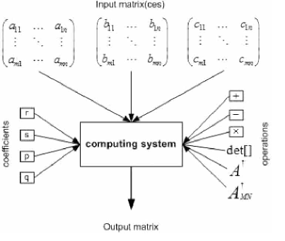
Figure 2: The matrix computation system

Each input matrix is, firstly, transformed into a string, with the elements separated by commas. Then the generated strings, subject to the required operations, are compared with data stored in the database. If the searching criteria are successfully ended, then a recomputation is not needed, and result will be displayed immediately in an appropriate web form.

The possibilities offered by the application are the following:

- unary operations: unary matrix operations, where only a single matrix and an optional coefficient is used to produce a unique result. ($A^{-1}$, $rA$, $A^{\dagger}$,…);

- binary operations: binary matrix operations, involving two matrices ($A+B$, $A^{p}\times B^{q}$,…);

- ternary operations: operations involving three matrices, such as the computation of the weighted Moore-Penrose inverse $A^{\dagger}_{MN}$.

User can define input matrices in two ways:

- by element-wise entering values for elements of the matrices;

- by uploading $txt$ file, which contains matrix entries, under the assumption that matrix rows match with lines of the file and matrix elements are separated with the blank character.

For this approach has been developed suitable Web interface illustrated in Figure 3.

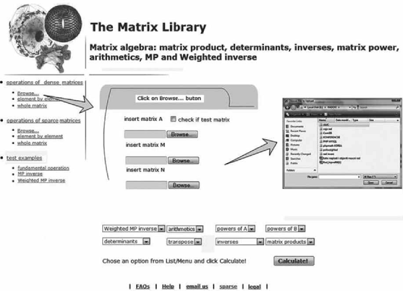
Figure 3: Web interface of the application

How does the application work? General algorithm is defined globally based on the next three steps.

The first step. The user chooses a matrix operation that will be implemented, via web browsers.

The second step. Select the type of matrix that will be proceeded and define entries. There are three types of matrices for processing: dense, sparse or test matrices. More, it is possible to define entries of the input matrix in one of the next three ways, as it is illustrated on Figure 4.

- loading the matrix from an existing textual file, using the button $Browse$. Matrix is stored in memory as $txt$ file, assuming that the elements of the matrix are separated with a comma, and the matrix rows are separated by the new line.

- entering the number of rows, columns and later values of the elements.

- entering a complete matrix in the text area box, assuming that its entries are separated by the blank character.

The third step: Generate and preview the solution.

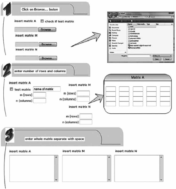
Figure 4: An example how to input matrix elements

All the once handled matrices, chosen operations and the generated results of processing are stored on the server in the appropriate form in txt files. In this way, it is possible to avoid recomputations and download solutions of previously performed operations. Users are also allowed to use ready-made test samples.

4 The Storage system

The matrices and their storage representations implemented in the paper can be classified in the following two groups.

Randomly generated and test matrices are stored in the database in two different storage systems. The row matrix format ($R$ format) assumes that all matrix elements are placed in a vector, so that the matrix is represented as a string containing values of the matrix elements separated by the comma. On the other hand, the $mR$ format represents a matrix in a database table under the assumption that the number of records in the table is equal to the number of rows of the matrix.

Sparse unstructured matrices are matrices whose entries are equal to zero for the most part and possess a distribution of the nonzero entries which do not match any specific pattern. There are various storage schemes, which minimize the memory space and computational requirements, by storing and performing arithmetic with only the nonzero elements. The simplest sparse matrix storage structure is the Coordinate Format ($COO$ format) [2], where the matrix is stored in three appropriate vectors, which represent the underlying sparse structure. The first vector (resp. the second vector) stores the row indices (resp. the column indices) for all non-zero entries. The third vector stores non-zero entries of the sparse matrix.

The $SQL$ codes for creating the data structure and tables on $MySQL$ database server are described as follows. The CREATE TABLE statement has three parts:

- A table name succeeds the $CREATE$ $TABLE$ statement.

- A list containing attribute names, types, and modifiers succeeds are placed between the parenthesis.

- A key list follows after the attribute list between the parenthesis.

In our implementation, we use only two different names for tables, namely $matrices\_in$ and $matrices\_out$;

⬇

# Table structure for table ‘matrices_in‘

CREATE TABLE matrices_in (

id_in int(11) NOT NULL auto_increment,

elements_in longtext NOT NULL,

dimension tinytext NOT NULL,

test tinytext NOT NULL,

sparse tinytext NOT NULL,

PRIMARY KEY (id_in)

) TYPE=MyISAM;

# Table structure for table ‘matrices_out‘

CREATE TABLE matrices_out (

id_out int(11) NOT NULL auto_increment,

elements_out longtext NOT NULL,

operation tinytext NOT NULL,

matrix_I int(11) NOT NULL default ’0’,

matrix_II int(11) NOT NULL default ’0’,

matrix_III int(11) NOT NULL default ’0’,

r tinyint(4) NOT NULL default ’0’,

s tinyint(4) NOT NULL default ’0’,

p tinyint(4) NOT NULL default ’0’,

q tinyint(4) NOT NULL default ’0’,

PRIMARY KEY (id_out)

) TYPE=MyISAM;

The fields used in the database tables are described as follows.

- $id\_in$ or $id\_out$: identification number, defined as $auto\_increment$;

- $elements\_in$ or $elements\_out$: string of type $longtext$, containing matrix entries separated with the comma character.

- $dimension$: string of the form ’$m$ x $n$’ which contains dimensions $m$ and $n$ of the matrix;

- $test$: string representing the name of a test matrix from [28], or the empty string (if the input matrix is not a test matrix);

- $sparse$: flag of type $tinytext$, possessing the value ’0’ if the matrix is non-sparse or one of the values, ’1’, ’2’, ’3’ for a sparse matrix; this field is important for searching the matrices already stored in the database;

- $operation$: It defines operations on input matrices ($A+B$, $rA+sB$, $A^{-1}+B^{-1}...$) or defines the computation of the weighted Moore-Penrose inverse;

- $matrix\_I$, $matrix\_II$ and $matrix\_III$: contain $IDs$ from the table $matrices\_in$ or default value ’0’ in order to find a solution for the chosen operation and entered matrices;

- $r$, $s$, $p$ and $q$: optional coefficients used to determine matrix operations $rA$, $sB$, $A^{p}$ and $B^{q}$, respectively.

It is clear that dimensions of matrices and vectors used as arguments are limited by the maximal length of the type $longtext$, which is within the interval $[0,2^{32}-1]$;

Example 4.1.

In the present example $matrix\_A$ defines the test matrix $A$ from [28] in the particular case $a=1$, $matrix\_B$ is randomly generated and the $matrix\_C$ is sparse and unstructured.

$$matrix\_A=\left[\begin{array}[]{cccccccccc}11&10&9&8&7&6&5&4&3&2\\ 10&10&9&8&7&6&5&4&3&2\\ 9&9&9&8&7&6&5&4&3&2\\ 8&8&8&8&7&6&5&4&3&2\\ 7&7&7&7&7&6&5&4&3&2\\ 6&6&6&6&6&6&5&4&3&2\\ 5&5&5&5&5&5&5&4&3&2\\ 4&4&4&4&4&4&4&4&3&2\\ 3&3&3&3&3&3&3&3&2&1\\ 2&2&2&2&2&2&2&2&1&0\\ 1&1&1&1&1&1&1&1&0&-1\\ \end{array}\right]_{11\times 10}$$

$$matrix\_B=\left[\begin{array}[]{cccccccccc}282&-11&-206&-39&84&94\\ -11&241&-80&129&121&-86\\ -206&-80&306&4&-113&2\\ -39&129&4&394&-19&-219\\ 84&121&-113&-19&119&15\\ 94&-86&2&-219&15&184\\ \end{array}\right]_{6\times 6}$$

$$matrix\_C=\left[\begin{array}[]{cccccccccc}1&2&3&0&0&0&0&0&0&0\\ 0&2&0&0&0&0&0&0&0&0\\ 1&0&0&4&0&0&0&0&0&0\\ 0&0&0&0&0&0&0&0&0&0\\ 0&4&0&0&0&8&0&0&0&0\\ 0&0&0&0&0&0&0&0&0&0\\ 0&0&0&0&0&0&0&0&0&0\\ 0&0&0&0&0&0&0&0&0&0\\ 0&0&0&0&0&0&0&0&0&0\\ 0&0&0&0&0&0&0&0&0&2\\ \end{array}\right]_{10\times 10}$$

The corresponding fragment of the table matrices_in is illustrated in Table 1.

$\bf matrices\_in$
$id\_in$	$elements\_in$	$dimension$	$test$	$sparse$
$1$	$11,10,9,...,1,1,1,0,-1$	$11\times 10$	$A\_10\_11$	0
2	282,-11,-206,…,2,-219,15,184	$6\times 6$	’ ’	0
3	0,0,0,1,2,2,4,4,9	$10\times 10$	’ ’	1
4	0,1,2,1,0,3,1,5,9	$10\times 10$	’ ’	2
5	1,2,3,2,1,4,4,8,2	$10\times 10$	’ ’	3

Table 1. Matrices in the database table $matrices\_in$

Three different matrices are stored in Table 1. The $matrix\_A$, which represents the test matrix $A_{11\times 10}$ from [28], is accommodated in the first row of the table. The representation of the $matrix\_B$ is placed in its second row. In the third, fourth and fifth rows is the sparse matrix representation for $matrix\_C$ in the $COO$ format.

The adjoint fragment of the table matrices_out is illustrated by Table 2, where $A(-1)$ and $A(MN)$ denote the inverse and the weighted Moore-Penrose inverse, respectively.

$\bf matrices\_out$
$id\_out$	$elements\_out$	$operation$	$matrix\_I$	$matrix\_II$	$matrix\_III$	$r$	$s$	$p$	$q$
1	1,-1,0,…,-0.25,-0.417	$A(-1)$	1	0	0	0	0	0	0
2	1974,-77,…,105,1288	$r*A+s*B$	2	2	0	3	4	0	0
3	0,0,0,0,1,2,2,2,4,9	$A*B$	3	3	0	0	0	0	0
4	0,1,2,3,1,0,1,2,1,9	$A*B$	4	4	0	0	0	0	0
5	4,6,3,12,4,1,2,3,8,4	$A*B$	5	5	0	0	0	0	0
4	0.755,-0.156,…,0.526,-0.2	$A(MN)$	18	14	17	0	0	0	0

Table 2. Matrices in database table $matrices\_out$

4.1 Relations between matrix representations and matrix storage systems

We present different methods for computing the pseudo-inverse $A^{\dagger}_{MN}$ and executing fundamental matrix operations, depending on the relationship between the implemented storage systems and matrix representations. As we have already mentioned, matrices are stored in the database in three formats: the $R$ format, the $mR$ format and the $COO$ format (only for the sparse matrix).

To accelerate the search of the resulting matrices stored in the database as well as to improve the pseudo-inverses computation, we exploit correlations between the presented storage systems indicated in Figure 5.

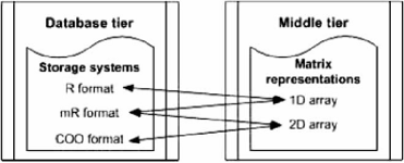
Figure 5: Relationship between storage systems and matrix representations

We implemented different computational systems for dense as well as for sparse matrices in order to detect the best. For dense matrices we use the computational systems illustrated on Figure 6. a. For sparse matrices we use a more suitable computational system, as shown on Figure 6. b.

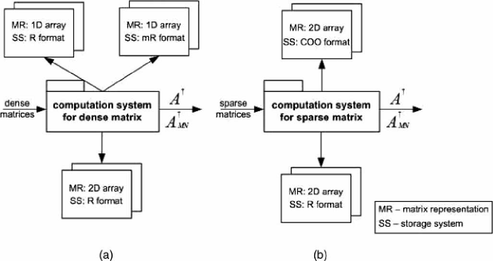
Figure 6: The computational systems for dense and sparse matrices

$UDFs$ for both dense and sparse matrices are implemented in the $2D$ array format. $UDFs$ for sparse matrices are adapted to $COO$ format storing system, opposite to $UDFs$ for dense matrices, which are adapted to $R$ format.

4.2 Implementation of matrix operations

Implementation of an arbitrary matrix operation in the database tier can be described by the following algorithm.

• 0:  Input matrices.

  1:  Define the input matrices and/or coefficients for processing and select the matrix operation.

  2:  Form the strings which define elements of entered matrices, applying Procedure 4.2 for each input (dense) matrix.

  3:  Search entered matrix in the database performing Procedure 4.3

  4:  ${\bf if}$ the input matrices and required operations exist in the database then

  5:      search the solution applying Procedure 4.5

  6:      ${\bf if}$ the solution exists then

  7:          $\bf{goto}$ Step 16

  8:       else

  9:          $\bf{goto}$ Step 14

  10:      ${\bf end}$ ${\bf if}$

  11:  else

  12:      Store entered matrix by applying Procedure 4.4 and goto Step 14.

  13:  ${\bf end}$ ${\bf if}$

  14:  Processing the input matrix executing Procedure 4.8.

  15:  Store the result performing Procedure 4.7.

  16:  return the result from the database using Procedure 4.6

   

We provide some procedures, applicable to dense matrices, that are used in our implementation.

Procedure 4.1.

Procedure 4.1 defines the input matrix by loading the corresponding $txt$ file. It can be used in Step 1 of Algorithm 4.2.

⬇

function upload_file(){

global $userfile,$userfile_name,$userfile_size,$userfile_type,$archive_dir,$WINDIR;

if(isset($WINDIR)) $userfile=$str_replace(”\\\\”,”\\”,$userfile);

$filename=basename($userfile_name);

if($userfile_size <= 0) die(”$filename is empty.”);

if(!@copy($userfile,”$archive_dir/$filename”))

die(”Can’t copy $userfile_name to $filename.”);

if (!isset($WINDIR)&&!@unlink($userfile))

die(”Can’t delete the file $userfile_name.”);}

Procedure 4.2.

Code used in Step 2 of Algorithm 4.2 for defining the string (vector) which includes entries of the dense matrix.

⬇

function make_vector($file){

$m=count($file);//number of rows

$string=””;

for($i=0;$i<$m;$i++){

$file[$i]=rtrim($file[$i]).”,”; $string=$string.$file[$i];}

$string1=$str_replace(” ”,”,”,$string);

$string2=substr($string1,0,strlen($string1)-1);//vector of all elements from matrix

return $string2;}

Procedure 4.3.

The searching of a dense matrix with randomly chosen elements is implemented by the next function. The search of a test matrix is defined by its unique name.

⬇

function if_exist($file){

$db_link=db_connect();//connect on the database

$m=m($file);//number of rows

$n=n($file);//number of columns

$dimension=$m.”x”.$n; $string2=make_vector($file);

$query=”select * from MATRICES_IN where DIMENSION=’$dimension’”;

$result=mysql_query($query,$db_link); $sum=0;

while($row=mysql_fetch_row($result)){

if($row[1]==$string2){$sum++; break;}}

if($sum==1){

$id_matrix=$row[0];}//matrix exist

else

$id_matrix=false;//matrix don’t exist

return $id_matrix;}

Procedure 4.4.

If the input matrix does not exist in the database, we store it applying the next code.

⬇

function enter_matrix($string2,$dimension,$test){

$db_link=db_connect();

$query=”insert into MATRICES_IN(ELEMENTS_IN,DIMENSION,TEST)

values(’$string2’,’$dimension’,’$test’)”;

$result=mysql_query($query,$db_link);}

Procedure 4.5.

If the entered matrices and operation already exist, we search the result from the database.

⬇

function result_exist($operation,$matrix1,$matrix2,$matrix3,$r,$s,$p,$q){

$db_link = db_connect();

$query = ”select * from MATRICES_OUT where OPERATION =’$operation’ and

MATRIX_I=’$matrix1’ and MATRIX_II=’$matrix2’ and MATRIX_III=’$matrix3’

and R=’$r’ and S=’$s’ and P=’$p’ and Q=’$q’”;

$result=mysql_query($query,$db_link);

$row=mysql_fetch_array($result);

if($row[1]==NULL){$matrix_out=false;}

else{$matrix_out=explode(”,”,$row[”ELEMENTS_OUT”]);}

return $matrix_out;}

Procedure 4.6.

If the result exists in the database table, we display it.

⬇

function presented_result($result,$m,$n){

for($i=0,$z=0;$i<$m;$i++){

for($j=0;$j<$n;$j++,$z++){

$result= round($result[$z],3);

echo ”<input name=elements[] type=text size=\”4\” maxlength=\”5\”

value=\”$result\” class=\”style21\” readonly=\”readonly\”> ”;}

echo ”<br>”;} }

Procedure 4.7.

The next code is aimed to store the result of the matrix manipulation.

⬇

function enter_solution($result,$operation,$id_m1,$id_m2,$id_m3,$r,$s,$p,$q){

$db_link=db_connect();

$string=implode($result,”,”);

$query=”insert into

MATRICES_OUT(ELEMENTS_OUT,OPERATION,MATRIX_I,MATRIX_II,MATRIX_III,R,S,P,Q)

values(’$string’,’$operation’,’$id_m1’,’$id_m2’,’$id_m3’,’$r’,’$s’,’$p’,’$q’)”;

$result=mysql_query($query,$db_link);}

4.3 The pseudo-inverse computation

The $Php$ code which implements the weighted Moore-Penrose inverse $A_{M,N}^{\dagger}$ according to Algorithm 2. Branching in the code is defined according to the selected storage system for our database table.

Procedure 4.8.

The main function for computation of the Weighted Moore-Penrose inverse.

⬇

function WeightedInverse($ArrayDataMatrixM,$ArrayDataMatrixA,$ArrayDataMatrixN){

$rows=count($ArrayDataMatrixA); $columns=count($ArrayDataMatrixA[0]);

$aa=ithCol(1,$ArrayDataMatrixA);

if(isZero($aa)==0)

$ar=Transpose($aa);

else{

$ta=Transpose($aa);

$alb=MultiplicationMatrices($ta,$ArrayDataMatrixM);

$ali=MultiplicationMatrices($alb,$aa);

$inv=Inverse($ali);

$ar=MultiplicationMatrices($inv,$alb);

}

for($i=2;$i<=$columns;$i++){

$ii=ithCol($i,$ArrayDataMatrixA);

$di=MultiplicationMatrices($ar,$ii);

$fc=frstiCol($i-1,$ArrayDataMatrixA);

$mm=MultiplicationMatrices($fc,$di);

$ci=SubsMatrices($ii,$mm);

$nim1=mMinus($ArrayDataMatrixN,$i);

$nim1g=Inverse($nim1);

$li=mColumn($ArrayDataMatrixN,$i);

if(isZero($ci)==0){

$nii=mskalar($ArrayDataMatrixN,$i);

$dit=Transpose($di);

$dtn=MultiplicationMatrices($dit,$nim1);

$dtnd=MultiplicationMatrices($dtn,$di);

$dtnd=matNum($dtnd);

$ditl=MultiplicationMatrices($dit,$li);

$lit=Transpose($li);

$litdi=MultiplicationMatrices($lit,$di);

$ditdi=SumaMatrices($ditl,$litdi);

$ditdi=matNum($ditdi);

$nim1li=MultiplicationMatrices($nim1g,$li);

$litnli=MultiplicationMatrices($lit,$nim1li);

$litnli=matNum($litnli);

$lktar=MultiplicationMatrices($lit,$ar);

$arnklk=MultiplicationMatrices($fc,$nim1li);

$novo=MultiplicationMatrices($lktar,$arnklk);

$novo=matNum($novo);

$si=$nii+$dtnd-$ditdi-$litnli+$novo;

$dtnar=MultiplicationMatrices($dtn,$ar);

$dilit=SubsMatrices($dtnar,$lktar);

$bit=ScalarMatrix($dilit,1/$si);

}

else{

$cit=Transpose($ci);

$citm=MultiplicationMatrices($cit,$ArrayDataMatrixM);

$pom=MultiplicationMatrices($citm,$ci); $pom=matNum($pom);

$bit=ScalarMatrix($citm,1/$pom);

}

$nim1li=MultiplicationMatrices($nim1g,$li);

$arai=MultiplicationMatrices($ar,$fc);

$arnim1=MultiplicationMatrices($arai,$nim1li);

$pi=SubsMatrices($nim1li,$arnim1);

$k1=MultiplicationMatrices($di,$bit);

$ark1=SubsMatrices($ar,$k1);

$pib=MultiplicationMatrices($pi,$bit);

$ar=SubsMatrices($ark1,$pib);

$ar=appRow($ar,$bit); }

return $ar;}

Implementation of previous function requires several auxiliary procedures.

Function ithCol generates the $i$th column a_i of $A$.

⬇

function ithCol($column,$ArrayDataMatrix1){

$rows1=count($ArrayDataMatrix1); $columns1=count($ArrayDataMatrix1[0]);

for($i=0;$i<$rows1;$i++) {

for($j=0;$j<$columns1;$j++){

if($j+1==$column)

$ArrayCol[$i][0]=$ArrayDataMatrix1[$i][$j]; } }

return $ArrayCol;}

The submatrix $A_{j}$=[a_1,…,a_j] which contains first $j\leq n$ columns of the matrix $A=A_{n}$=[a_1,…,a_n] can be generated performing the next function:

⬇

function frstiCol($columns,$ArrayDataMatrix1){

$rows1=count($ArrayDataMatrix1); $columns1=count($ArrayDataMatrix1[0]);

for($i=0;$i<$rows1;$i++){

for($j=0;$j<$columns1;$j++){

if($j+1<=$columns)

$ArrayCol[$i][$j]=$ArrayDataMatrix1[$i][$j];} }

return $ArrayCol;}

Procedure matNum() converts matrix of dimension $1\times 1$ into the number.

⬇

function matNum($ArrayDataMatrix1){

$rows1=count($ArrayDataMatrix1); $columns1=count($ArrayDataMatrix1[0]);

if($rows1==1&$columns1==1)

return $ArrayDataMatrix1[0][0];}

Function isZero() checks whether the parameter is zero matrix or not.

⬇

function isZero($ArrayDataMatrix1){

$isZero=0; $rows1=count($ArrayDataMatrix1); $columns1=count($ArrayDataMatrix1[0]);

for($i=0;$i<$rows1;$i++){

for($j=0;$j<$columns1;$j++){

if(round($ArrayDataMatrix1[$i][$j],3)!=0)

$isZero++; } }

return $isZero;}

Function appRow() appends the column vector $Y$ to the matrix $X$.

⬇

function appRow($ArrayDataMatrix1,$ArrayDataMatrix2){

$isZero=0;

$rows1=count($ArrayDataMatrix1);

$columns2=count($ArrayDataMatrix2[0]);

for($i=0;$i<$columns2;$i++){

$ArrayDataMatrix1[$rows1][$i]=$ArrayDataMatrix2[0][$i];}

return $ArrayDataMatrix1;}

Finally, the function Inverse() returns the inverse of the input parameter.

⬇

function Inverse($ArrayDataMatrix){

$rows=count($ArrayDataMatrix); $columns=count($ArrayDataMatrix[0]);

$nii=mskalar($ArrayDataMatrix,1);

$N=1/$nii; $N=array(array($N));

for($i=2;$i<=$columns;$i++){

$s=mskalar($ArrayDataMatrix,$i);

$nii=array(array($s));

$li=mColumn($ArrayDataMatrix,$i);

$lit=Transpose($li);

$giip=MultiplicationMatrices($lit,$N);

$gii1=MultiplicationMatrices($giip,$li);

$gii=SubsMatrices($nii,$gii1);

$gii2=matNum($gii); $gii=1/$gii2;

$fip=MultiplicationMatrices($N,$li);

$fi1=ScalarMatrix($fip,$gii);

$fi=ScalarMatrix($fi1,-1);

$fit=Transpose($fi);

$E1=MultiplicationMatrices($fi,$fit);

$E2=ScalarMatrix($E1,1/$gii);

$E=SumaMatrices($N,$E2);

$ArrayDataMatrix1=appRow($E,$fit);

$giin=array(array($gii));

$ArrayDataMatrix2=appRow($fi,$giin);

$N=finaly($ArrayDataMatrix1,$ArrayDataMatrix2); }

return $N;}

5 Examples

Example 5.1.

In the next table, we compare the CPU time spent for searching the matrices stored in the database by two different storage systems.

Search of stored matrices
number of matrices	$R$ format	$mR$ format
$50$	0.102 sec.	0.647 sec.
$100$	0.166 sec.	0.660 sec.
$500$	0.7909 sec.	14.079 sec.
$1000$	1.901 sec.	28.650 sec.

Table 3. The CPU time for searching matrices dimension $70\times 70$ in the $R$ and $mR$ format.

This testing is performed for dense matrices with randomly chosen elements. from Table 3. we conclude that the CPU time for searching is much shorter when the $R$ format is used.

Let us mention that the searching of the test matrices from [28] is based on the search by a unique name, and does not depend on the number of the matrices stored in the database.

Example 5.2.

In Table 4. are arranged $CPU$ times required for computation of the pseudo-inverse $A^{\dagger}_{MN}$. Matrices are represented in two different ways: as $1D$ arrays based on the $mR$ and $R$ format, or in the form of $2D$ arrays combined with the $R$ format storage system.

$A^{\dagger}_{MN}$
matrix representation: storage system
$m\times n$	1D array: $mR$ format	1D array: $R$ format	2D array: R format
$A\_30\_3$	4.485 sec.	2.440 sec.	0.897 sec.
$A\_50\_4$	32.834 sec.	21.270 sec.	6.199 sec.
$F\_15\_2$	0.666 sec.	0.342 sec.	0.166 sec.
$F\_30\_3$	4.379 sec.	2.347 sec.	0.880 sec.
$F\_50\_4$	32.564 sec.	20.981 sec.	6.077 sec.
$S\_50\_4$	32.597 sec.	20.874 sec.	6.070 sec.
$S\_80\_5$	269.282 sec.	206.007 sec.	40.75 sec.
$50\times 50$	32.423 sec.	21.294 sec.	6.203 sec.
$15\times 15$	0.632 sec.	0.471 sec.	0.160 sec.
$50\times 35$	9.79 sec.	5.587 sec.	1.997 sec.
$45\times 70$	125.18 sec.	86.210 sec.	19.920 sec.
$60\times 60$	70.260 sec.	49.964 sec.	12.627 sec.

Table 4. Computation time for $A^{\dagger}_{MN}$ when matrices don’t exist in the database.

Results of the testing show that the best processing time is achieved in the case when matrices are presented in the form of $2D$ arrays.

Example 5.3.

In this example, we compare the CPU times obtained during the computation of the pseudo-inverse $A^{\dagger}_{MN}$ (in the case when the input matrices are not stored in the database) with the CPU times required for searching the same results (in the case when the input matrices are stored in the database). Matrices are presented in $2D$ array representation, $R$ format storage system.

A${}^{\dagger}_{MN}$
matrix representation: storage system
$m\times n$	$2D$ $array:Rformat$ (exist)	$2D$ $array:Rformat$ (don’t exist)
$20\times 20$	0.043 sec.	0.309 sec.
$30\times 30$	0.051 sec.	2.105 sec.
$45\times 45$	0.062 sec.	4.665 sec.
$50\times 50$	0.070 sec.	6.729 sec.
$60\times 60$	0.075 sec.	12.675 sec.
$70\times 70$	0.079 sec.	26.614 sec.
$80\times 80$	0.096 sec.	43.809 sec.

Table 5. The CPU time for $A^{\dagger}_{MN}$ when matrices exist and don’t exist in the database.

The CPU time required for searching the solution from the database is negligible with respect to the time needed for the recalculation, especially if the matrix has larger dimensions. Let us mention that 10030 records are stored in the table $matrices\_in$ at the moment of testing.

Example 5.4.

Comparison of the $CPU$ time for executing fundamental matrix operations is given in Table 6.

Fundamental operation on matrices
$m\times n$		$operation$	$1D$ $format$: $Rformat$	2D array: $Rformat$
$3\times 3$	$3\times 3$	multiplication	0.0468 sec.	0.0043 sec.
$5\times 5$	$5\times 5$	multiplication	0.0481 sec.	0.0042 sec.
$10\times 10$	$10\times 10$	multiplication	0.0643 sec.	0.0062 sec.
$20\times 50$	$50\times 50$	multiplication	0.1531 sec.	0.0778 sec.
$45\times 45$	$45\times 70$	multiplication	0.5618 sec.	0.1369 sec.
$80\times 80$	$80\times 60$	multiplication	0.9325 sec.	0.7270 sec.
$80\times 70$	$70\times 70$	multiplication	0.9675 sec.	0.5600 sec.
$81\times 81$	$81\times 81$	multiplication	1.2831 sec.	0.7470 sec.
$3\times 3$	$3\times 3$	addition	0.0425 sec.	0.0040 sec.
$5\times 5$	$5\times 5$	addition	0.0431 sec.	0.0043 sec.
$10\times 10$	$10\times 10$	addition	0.0431 sec.	0.0048 sec.
$50\times 50$	$50\times 50$	addition	0.1400 sec.	0.0326 sec.
$60\times 60$	$60\times 60$	addition	0.2012 sec.	0.0480 sec.
$70\times 70$	$70\times 70$	addition	0.2481 sec.	0.0705 sec.
$80\times 80$	$80\times 80$	addition	0.3287 sec.	0.0919 sec.
$3\times 3$	$3\times 3$	substraction	0.0475 sec.	0.0041 sec.
$5\times 5$	$5\times 5$	substraction	0.0512 sec.	0.0044 sec.
$10\times 10$	$10\times 10$	substraction	0.0350 sec.	0.0050 sec.
$50\times 50$	$50\times 50$	substraction	0.1431 sec.	0.0319 sec.
$60\times 60$	$60\times 60$	substraction	0.1875 sec.	0.0733 sec.
$70\times 70$	$70\times 70$	substraction	0.2512 sec.	0.0415 sec.
$81\times 81$	$81\times 81$	substraction	0.3150 sec.	0.1196 sec.

Table 6. The CPU time for $1D$ array and $2D$ array in $R$ format processing.

The arranged results show that the smallest computational time is obtained in the case when the matrix is presented in the format of $2D$ array, $R$ format storage system.

Testing was done on the local machine and from client in a wireless network. We had an access to the web server using the infrastructure mode wireless networking with an access point. Testing was executed on the server machine with: Windows edition: $Windows$ $Vista^{(TM)}$ $Ultimate$; Processor: $Intel(R)$ $Pentium(R)$ $Dual$ $CPU$ $T3200\ @\ 2.00GHz$; Memory $(RAM):2940MB$; System type: $32-bit\ Operating\ System$; Free Software: $WAMP$ $5$ $1.7.4$ installs: $PHP\ 5.2.5$, $Apache\ 2.2.6$ $Server$, $MySQL\ 5.0.45$ and $phpMyAdmin\ 2.11.2.1$.

The $CPU$ time shows that searching of a matrix which is given in the $R$ format gives better results than the searching of the same matrix presented in the $mR$ format. Furthermore, the best results are obtained in the case when matrices are represented in view of the two-dimensional arrays (on the middle tier), application logic adapted to the $R$ format, and matrices are stored in the $R$ format in the database. Searching time is inversely proportional with the number of data transferred between the middle of the application tier and the database tier.

6 Conclusions

This research contributes to the development of an $OSS$ application and construction of the matrix library, especially in computation of the generalized inverses. Several storage technics are discussed and tested in the $PHP/MySQL$ environment. Data’s preparation as an important preprocessing step of data mining is a further application for database matrix computations. There are several issues for future work. We plan to develop mechanisms which decrease memory usage and minimize the searching time in accordance with different storage systems. Furthermore, it is possible to adapt $UDF$s to sparse structured matrices, such as diagonal matrices, sparse symmetric matrices, triangular matrices, Toeplitz matrices, etc. We need to identify other mathematical operations with wide applicability that can be implemented with the $PHP/MySQL$ environment, thereby enhancing the $DBMS$ data mining functionality. Also, further implementation of the matrix library will be based on the principles of $Object$-$Oriented$ $Programming$.

References

- [1] J. Clear, D. Dunn, B. Harvey, M.L. Heytens, and P. Lohman, Non-stop SQL/MX primitives for knowledge discovery, In ACM KDD Conference, (1999) 425- 429.
- [2] T. Chong, Shamik D. Sharma, E. Brewer and J. Saltz, Sparse matrix application, Parallel Processing Letters. Volume 5, Number 4 (1995), 671–683.
- [3] S. Egilsson, H. Gudbjartsson and S. Sigurjnsson, SQL query generator utilizing matrix structures, U.S. Patent 6,578,028, Jun 10, 2003.
- [4] R. Elmasri and S.B. Navathe, Fundamentals of Database Systems, Addison-Wesley, 4th edition, 2003.
- [5] J. Greenspan and B. Bulger, MySQL/PHP Database Applications M&T Books: An imprint of IDG Books Worldwide, Inc., 2001.
- [6] T. N. E., Grevile, Some applications of the pseudo-inverse of matrix SIAM Rev. 3 (1960), 15–22.
- [7] C. Itiki, Dynamic programming and diagnostic classification, J. Optim. Theory Appl. 127 (2005), 579 -586.
- [8] E. Karaman and E. Kayhan, A client server based model for parallel matrix computation, SIAM Rev. 3 (1960), 15–22.
- [9] T. Kurmayya and K.C. Sivakumar, Moore-Penrose inverse of a Gram matrix and its nonnegativity, J. Optim. Theory Appl., 139 (2008), 201 -207.
- [10] S.Y.T. Lee, H.W. Kim and S. Gupta, Measuring open source software success, OMEGA-Int. J. Manage S. 37 (2009), 426–438.
- [11] J.B. Layton, Efficient direct computation of the pseudo-inverse and its gradient, Internat. J. Numer. Methods Engrg. 40 (1997), 4211–4223.
- [12] J. Meloni, PHP 5, MA: Thomson Course Techology, Boston, 2004.
- [13] S. Mohideen and V. Cherkassky, On recursive calculation of the generalized inverse of a matrix, ACM Trans. Math. Software 17 (1991), 130 -147.
- [14] J.C. Nash and R.L.C. Wang, Algorithm 645 Subroutines for testing programs that compute the generalized inverse of a matrix, ACM Trans. Math. Software 12 (1986), 274–277.
- [15] C. Ordonez and J. García, Vector and matrix operations programmed with UDFs in a relational DBMS, Proceedings of the 15th ACM international conference on Information and knowledge management, Arlington, Virginia, USA. 2006, 503–512.
- [16] R. Page and P. Factor, SQL Server Matrix Workbench, (2008) Web site: http://www.simple-talk.com/sql/t-sql-programming/sql-server-matrix-workbench/.
- [17] M. D. Petković, P.S. Stanimirović and M.B. Tasić, Effective partitioning method for computing weighted Moore Penrose inverse, Comput. Math. Appl. 55 (2008), 1720- 1734.
- [18] M.D. Petković and P.S. Stanimirović, Symbolic computation of the Moore-Penrose inverse using partitioning method, Int. J. Comput. Math. 82 (2005), 355–367.
- [19] P. S. Stanimirović and M.B. Tasić, Partitioning method for rational and polynomial matrices, Appl. Math. Comput. 155 (2004), 137–163.
- [20] P.S. Stanimirović and M.B. Tasić, A problem in computation of pseudoinverses, Appl. Math. Comput. 135 (2003), 443–469.
- [21] P.S. Stanimirović and M.B. Tasić, Computing generalized inverses using LU factorization of matrix product, Int. J. Comput. Math. 85 (2008), 1865- 1878.
- [22] M. B. Tasić, P.S. Stanimirović and M.D. Petković, Symbolic computation of weighted Moore-Penrose inverse using partitioning method, Appl. Math. Comput. 155 (2004), 137–163.
- [23] M. B. Tasić, P. S. Stanimirović and S. H. Pepić, About the generalized LM-inverse and the weighted Moore Penrose inverse, Appl. Math. Comput. 216 (2010), 114- 124.
- [24] M. B. Tasić, P. S. Stanimirović, Differentiation of generalized inverses for rational and polynomial matrices, Appl. Math. Comput. 216 (2010), 2092 -2106.
- [25] F.E. Udwadia and R.E. Kalaba, Analytical Dynamics: A New Approach, Cambridge University Press, Cambridge, England, 1996.
- [26] G. R. Wang and Y.L.Chen, A recursive algorithm for computing the weighted Moore-Penrose inverse , J. Comput. Math. 4 (1986), 74–85.
- [27] H. E. Williams and D. Lane, Web Database Applications with PHP and MySQL, O’Reilly & Associates, Inc., 2002.
- [28] G. Zielke, Report on test matrices for generalized inverses, Computing 36 (1986), 105–162.