Statistics of reflection eigenvalues in chaotic cavities with non-ideal leads

Abstract

The scattering matrix approach is employed to determine a joint probability density function of reflection eigenvalues for chaotic cavities coupled to the outside world through both ballistic and tunnel point contacts. Derived under assumption of broken time-reversal symmetry, this result is further utilised to (i) calculate the density and correlation functions of reflection eigenvalues, and (ii) analyse fluctuations properties of the Landauer conductance for the illustrative example of asymmetric chaotic cavity. Further extensions of the theory are pinpointed.

Introduction.—At low temperatures and voltages, a phase coherent charge transfer through quantum chaotic cavities is known to exhibit a high degree of statistical universality B-1997 ; A-2000 . Even though the transport through an individual chaotic structure is highly sensitive to its microscopic parameters, the universal statistical laws emerge upon appropriate ensemble or energy averaging procedure. The latter efficiently washes out all system-specific features provided a charge carrier has stayed in a cavity long enough to experience diffraction AL-1996 ; RS-2002 . Quantitatively, this requires the average electron dwell time $\tau_{\rm D}$ to be in excess of the Ehrenfest time $\tau_{\rm E}$ that defines the time scale where quantum effects set in.

In the extreme limit $\tau_{\rm D}\gg\tau_{\rm E}$, the statistics of charge transfer is shaped by the underlying symmetries B-1997 of a scattering system (such as the absence or presence of time-reversal, spin-rotational, and/or particle-hole symmetries). For this reason, a stochastic approach LW-1991 based on the random matrix theory M-2004 (RMT) description BGS-1984 of electron dynamics in a cavity is naturally expected to constitute an efficient framework for nonperturbative studies of the universal transport regime. Indeed, a stunning progress was achieved in the RMT applications to the transport problems over the last two decades. Yet, intensive research in the fieldBFS-2011 left unanswered many basic-level questions. One of them, regarding the statistics of transmission/reflection eigenvalues in chaotic cavities coupled to the leads through the point contacts with tunnel barriers, will be a focus of this Letter.

Supported by the supersymmery field theoretic technique E-1997 as well as by recent semiclassical studies RS-2002 , the RMT approach to quantum transport starts with the Heidelberg formula for the scattering matrix MW-1963

$${\bm{\mathcal{S}}}(\varepsilon_{F})=\openone_{N}-2i\pi{\bm{\mathcal{W}}}^{\dagger}({\varepsilon}_{F}\,\openone_{M}-{\bm{\mathcal{H}}}+i\pi{\bm{\mathcal{W}}}{\bm{\mathcal{W}}}^{\dagger})^{-1}{\bm{\mathcal{W}}}$$ (1)

of the total system comprised by the cavity and the leads. Here, an $M\times M$ random matrix ${\bm{\mathcal{H}}}$ (of proper symmetry, $M\rightarrow\infty$) models a single electron Hamiltonian whilst an $M\times N$ deterministic matrix ${\bm{\mathcal{W}}}$ describes the coupling of electron states with the Fermi energy ${\varepsilon_{F}}$ in the cavity to those in the leads; $N=n_{\rm L}+n_{\rm R}$ is the total number of propagating modes (channels) in the left ($n_{\rm L}$) and right ($n_{\rm R}$) leads. Equation (1) refers to chaotic cavities with sufficiently large capacitance (small charging energy) when the electron-electron interaction can be disregarded B-1997 . Throughout the paper, only such cavities are considered.

Landauer’s insight LFLB-1957 that electronic conduction in solids can be thought of as a scattering problem makes the $N\times N$ scattering matrix ${\bm{\mathcal{S}}}(\varepsilon_{F})$ a central player in statistical analysis of various transport observables. In the physically motivated $M\rightarrow\infty$ scaling limit, its distribution, dictated solely by the symmetries of the random matrix $\bm{\mathcal{H}}$, is well studied for both normal B-1995 and normal-superconducting B-2009 chaotic systems. In the former case, the distribution of ${\bm{\mathcal{S}}}(\varepsilon_{F})$ is described by the Poisson kernel H-1963 ; B-1995

$$P_{\beta}({\bm{\mathcal{S}}})\propto\big{[}{\rm det}(\openone_{N}-\bar{\bm{\mathcal{S}}}{\bm{\mathcal{S}}}^{\dagger})\,{\rm det}(\openone_{N}-{\bm{\mathcal{S}}}\bar{\bm{\mathcal{S}}}^{\dagger})\big{]}^{\beta/2-1-\beta N/2}.$$ (2)

Here, $\beta$ is the Dyson index M-2004 accommodating system symmetries: ${\bm{\mathcal{S}}}(\varepsilon_{F})$ is unitary symmetric for $\beta=1$, unitary for $\beta=2$, and unitary self-dual for $\beta=4$. All relevant microscopic details of the scattering system are encoded into a single average scattering matrix

$$\bar{\bm{\mathcal{S}}}=(M\Delta\openone_{N}-\pi^{2}{\bm{\mathcal{W}}}^{\dagger}{\bm{\mathcal{W}}})\,(M\Delta\openone_{N}+\pi^{2}{\bm{\mathcal{W}}}^{\dagger}{\bm{\mathcal{W}}})^{-1},$$ (3)

where $\Delta$ denotes the mean level spacing at the Fermi level in the limit $M\rightarrow\infty$. The $N$ eigenvalues $\hat{\bm{\gamma}}={\rm diag}(\{\sqrt{1-\Gamma_{j}}\})$ of $\bar{\bm{\mathcal{S}}}$ characteriseB-1997 couplings between the cavity and the leads in terms of tunnel probabilities $\Gamma_{j}$ of the $j$-th electron mode in the leads. The celebrated result Eq. (2), that can be viewed as a generalisation of the three Dyson circular ensembles M-2004 , was alternatively derived through a phenomenological information-theoretic approach reviewed in Ref. MB-1999 .

Unfortunately, statistical information accommodated in the Poisson kernel is too detailed to make a nonperturbative description of transport observables operational. It turns out, however, that in case of conserving charge transfer through normal chaotic structures, it is suffice to know a probability measure associated with a set ${\bm{T}}$ of non-zero transmission eigenvalues $\{T_{j}\in(0,1)\}$; these are the eigenvalues of the Wishart-type matrix ${\bm{t}}{\bm{t}}^{\dagger}$, where ${\bm{t}}$ is the transmission sub-block of the scattering matrix

$$\bm{{\mathcal{S}}}=\left(\begin{array}[]{cc}{\bm{r}}_{n_{\rm L}\times n_{\rm L}}&{\bm{t}}_{n_{\rm L}\times n_{\rm R}}\\ {\bm{t}^{\prime}}_{n_{\rm R}\times n_{\rm L}}&{\bm{r}^{\prime}}_{n_{\rm R}\times n_{\rm R}}\\ \end{array}\right).$$ (6)

Owing to this observation, the joint probability density function $P_{\beta}({\bm{T}})$ emerges as the object of primary interest in the RMT theories of quantum transport.

Surprisingly, our knowledge of the probability measure $P_{\beta}({\bm{T}})$ induced by the Poisson kernel [Eq. (2)] is very limited, being restricted to chaotic cavities coupled to external reservoirs via ballistic point contactsvHB-1996 (“ideal leads”). In this, mathematically simplest case, the unity tunnel probabilities $\Gamma_{j}=1$ make the average scattering matrix $\bar{\bm{\mathcal{S}}}$ vanish, giving rise to the uniformly distributedBS-1990 scattering matrices which otherwise maintain a proper symmetryM-2004 . In the RMT language, this implies that scattering matrices belong to one of the three Dyson circular ensemblesD-1962 .

As was first shown by Baranger and MelloBM-1994 , and by Jalabert, Pichard, and BeenakkerJPB-1994 , the uniformity of scattering matrix distribution induces a nontrivial joint probability density function of transmission eigenvalues $\{T_{j}\}$ of the formF-2006

$$P_{0}^{(\beta)}({\bm{T}})\propto\,|\Delta_{n}^{\beta}({\bm{T}})|\prod_{j=1}^{n}T_{j}^{\beta/2-1+\beta\nu/2}.$$ (7)

Here, $\nu=|n_{\rm L}-n_{\rm R}|$ is the asymmetry parameter, $n={\rm min}(n_{\rm L},n_{\rm R})$ is the number of non-zero eigenvalues of the matrix ${\bm{t}}{\bm{t}}^{\dagger}$, whilst $\Delta_{n}({\bm{T}})$ is the Vandermonde determinant $\Delta_{n}({\bm{T}})=\prod_{j<k}(T_{k}-T_{j})$. Equation (5) is one of the cornerstones of the RMT approach to quantum transport.

From ballistic to tunnel point contacts.—The restricted validity of Eq. (7), that holds true for chaotic cavities with ideal leads, is hardly tolerable both theoretically (an important piece of the transport theory is missing R-previous ) and experimentally (chaotic structures with adjustable point contacts, including tunable tunnel barriers, can by now be fabricatedKMR-1997 ). In this Letter, a first systematic foray is made into a largely unexplored territory of non-ideal couplings. In doing so, we choose (for the sake of simplicity) to lift a point-contact-ballisticity only for the left lead which is assumed to support $n_{\rm L}$ propagating modes characterised by a set of tunnel probabilities $\hat{{\bm{\Gamma}}}_{\rm L}=(\Gamma_{1},\dots,\Gamma_{n_{\rm L}})$; the right lead, supporting $n_{\rm R}\geq n_{\rm L}$ open channelsR-01 , is kept ideal so that $\hat{{\bm{\Gamma}}}_{\rm R}=(\Gamma_{n_{\rm L}+1},\dots,\Gamma_{n_{\rm R}})=\openone_{n_{\rm R}-n_{\rm L}}$. Assuming that the time-reversal symmetry is broken ($\beta=2$), we shall show that the joint probability density function $P_{(\hat{{\bm{\gamma}}}_{\rm L}|\,{\bm{0}})}({\bm{R}})$ of reflection eigenvalues $\{R_{j}=1-T_{j}\}$ equalsR-01a

$$P_{(\hat{{\bm{\gamma}}}_{\rm L}|\,{\bm{0}})}(R_{1},\dots,R_{n_{\rm L}})=c_{n_{\rm L},n_{\rm R}}\,\frac{{\rm det}{}^{N}(\openone_{n_{\rm L}}-\hat{{\bm{\gamma}}}_{\rm L}^{2})}{\Delta_{n_{\rm L}}(\hat{{\bm{\gamma}}}_{\rm L}^{2})}\,\Delta_{n_{\rm L}}({\bm{R}})\,{\rm det}_{(j,k)\in(1,n_{\rm L})}\Big{[}{}_{2}F_{1}(n_{\rm R}+1,n_{\rm R}+1;1;\,\gamma_{j}^{2}R_{k})\Big{]}\prod_{j=1}^{n_{\rm L}}(1-R_{j})^{\nu}.$$ (8)

Here, $\hat{{\bm{\gamma}}}_{\rm L}^{2}=\openone_{n_{\rm L}}-\hat{{\bm{\Gamma}}}_{\rm L}$ is a set of $n_{\rm L}$ coupling parameters characterising non-ideality of the left lead in terms of associated tunnel probabilities, $N=n_{\rm L}+n_{\rm R}$ is the total number of open channels in both leads, $c_{n_{\rm L},n_{\rm R}}$ is the inverse normalisation constant,

$$c_{n_{\rm L},n_{\rm R}}=\frac{(n_{\rm L}+n_{\rm R})!}{n_{\rm L}!\,n_{\rm R}!}\prod_{j=1}^{n_{\rm L}}\frac{(n_{\rm R}!)^{2}}{(n_{\rm R}+j)!\,(n_{\rm R}-j)!},$$ (9)

whilst ${}_{p}F_{q}$ is the Gauss hypergeometric function. The (biorthogonal DF-2008 ) ensemble of reflection eigenvalues Eq. (8) is our first main resultRemark0 . Before outlining its derivation, let us discuss the implications of Eq. (8) for a nonperturbative statistical description of both spectral and transport observables in quantum chaotic cavities.

Statistics of reflection eigenvalues.—The first immediate consequence of Eq. (8) is the determinant structure of the $p$-point correlation function of reflection eigenvalues:

$$\rho_{(n_{\rm L},n_{\rm R})}(R_{1},\dots,R_{p})={\rm det}_{(j,k)\in(1,p)}\left[K_{(n_{\rm L},n_{\rm R})}(R_{j},R_{k})\right].$$ (10)

Defined in a standard mannerM-2004 , it is entirely determined by the two-point scalar kernel $K_{(n_{\rm L},n_{\rm R})}(R,R^{\prime})$, that can straightforwardly be calculated VK-2011 by applying the ideas exposed in Ref.DF-2008 . In terms of the “moment function”

$$M_{k}^{(\nu)}(\gamma^{2})=\sum_{\ell=0}^{\nu}(-1)^{\ell}\left(\genfrac{}{}{0.0pt}{}{\nu}{\ell}\right)\,M_{k+\ell}^{(0)}(\gamma^{2}),$$ (11)

where $M_{k}^{(0)}(\gamma^{2})=k^{-1}\,{}_{3}F_{2}(n_{\rm R}+1,n_{\rm R}+1,k;1,k+1;\gamma^{2})$, the scalar kernel is given by a finite sum:

$$K_{(n_{\rm L},n_{\rm R})}(R,R^{\prime}) = n_{\rm L}!\,c_{n_{\rm L},n_{\rm R}}\,\frac{{\rm det}^{n_{\rm L}+n_{\rm R}}(\openone_{n_{\rm L}}-\hat{{\bm{\gamma}}}_{\rm L}^{2})}{\Delta_{n_{\rm L}}(\hat{{\bm{\gamma}}}_{\rm L}^{2})}\,[(1-R)(1-R^{\prime})]^{\nu/2}$$

$$\times \,\sum_{j=1}^{n_{\rm L}}{}_{2}F_{1}(n_{\rm R}+1,n_{\rm R}+1,1;\gamma_{j}^{2}R)\,{\rm det}\left[[M_{k}^{(\nu)}(\gamma_{\ell}^{2})]_{\ell=1,\cdots,j-1};\,(R^{\prime})^{k-1};\,[M_{k}^{(\nu)}(\gamma_{\ell}^{2})]_{\ell=j+1,\cdots,n_{\rm L}}\right].$$

Here, $k\in(1,n_{\rm L})$ counts the rows of an $n_{\rm L}\times n_{\rm L}$ matrix under the sign of determinant. Equations (10) and (Statistics of reflection eigenvalues in chaotic cavities with non-ideal leads) represent our second main result.

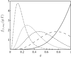
Figure 1: Probability density function $f_{(1,n_{\rm R})}(g;\Gamma)$ for Landauer conductance plotted for $n_{\rm R}=5$ and various tunnel probabilities: $\Gamma=0.99$ (solid line), $\Gamma=0.8$ (long-dashed line), $\Gamma=0.6$ (dashed line), $\Gamma=0.4$ (dotted line), and $\Gamma=0.2$ (dot-dashed line). For the ideal point contact ($\Gamma=1$), the curve is a monotonous function of $g$ reaching its maximum at $g_{*}=1$. Decrease of the tunnel probability leads to development of a well-pronounced maximum. In the large-$n_{\rm R}$ limit, it is positioned at $g_{*}=\Gamma$, see Eq. (14).

Distribution of Landauer conductance.—Although the central result of this Letter, Eq. (8), allows us to address the problem of conductance fluctuations in full generality, the most explicit formulae can be obtained for the illustrative example of an asymmetric cavity whose left (non-ideal) lead supports a single propagating mode ($n_{\rm L}=1$). For such a setup, a probability density $f_{(1,n_{\rm R})}(g;\Gamma)$ of the Landauer conductance is proportional to the mean density $K_{(1,n_{\rm R})}(R,R)$ of reflection eigenvalues taken at $R=1-g$. Materialising this observation with the help of Eq. (Statistics of reflection eigenvalues in chaotic cavities with non-ideal leads), we derive R-particular :

$$f_{(1,n_{\rm R})}(g;\Gamma)=f_{(1,n_{\rm R})}(g;1)\,\Gamma^{n_{\rm R}+1}\qquad\qquad\qquad\qquad$$

$$\times\,{}_{2}F_{1}(n_{\rm R}+1,n_{\rm R}+1;1;\,(1-\Gamma)(1-g)).\quad$$ (13)

Here, $\Gamma$ is the tunnel probability of the left point contact, whilst $f_{(1,n_{\rm R})}(g;1)=n_{\rm R}g^{n_{\rm R}-1}$ describes the conductance density when the left point contact is ballistic.

The probability density of Landauer conductance Eq. (Statistics of reflection eigenvalues in chaotic cavities with non-ideal leads) shows an unusually rich behavior (see Fig. 1). First, it exhibits a pronounced maximum whose position $g_{*}$, for a generic value of the tunnel probability $\Gamma$, depends on the number ($n_{\rm R}$) of propagating modes in the ideal lead. Second, numerical analysis of Eq. (Statistics of reflection eigenvalues in chaotic cavities with non-ideal leads) reveals existence of a “critical” value ($\Gamma_{0}$) of the tunnel probability: for $\Gamma<\Gamma_{0}$, increase of $n_{\rm R}$ makes the maximum position move from left to right until it approaches its saturated location $g_{*}=\Gamma$; on the contrary, for $\Gamma>\Gamma_{0}$, as $n_{\rm R}$ increases, position of the maximum moves in the opposite direction eventually reaching $g_{*}=\Gamma$.

To describe this effect analytically, one has to seek an explicit functional form of $g_{*}(\Gamma,n_{\rm R})$ for arbitrary $\Gamma$ and $n_{\rm R}$, which appears to be an impossible task. However, some progress can be made in the large-$n_{\rm R}$ limit, when an $1/n_{\rm R}$ expansion can be developed. A somewhat cumbersome calculation VK-2011 based on the asymptotic analysis of the hypergeometric function in Eq. (Statistics of reflection eigenvalues in chaotic cavities with non-ideal leads) brings out the remarkable formula

$$g_{*}(\Gamma,n_{\rm R})=\Gamma\left[1+\frac{7}{2n_{\rm R}}\left(\Gamma-\frac{6}{7}\right)+O(n_{\rm R}^{-2})\right],$$ (14)

suggesting that the “critical” value $\Gamma_{0}$ of the tunnel probability equals $\Gamma_{0}=6/7$. This prediction is unequivocally supported by numerics based on the exact Eq. (Statistics of reflection eigenvalues in chaotic cavities with non-ideal leads), see Fig. 2. We believe that experimental testing of the “$6/7$” effect may be feasible within the current limits of nanotechnology E-2001 .

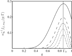
Figure 2: Unnormalised conductance “distribution” $n_{\rm R}^{-1}f_{(1,n_{\rm R})}(g;\Gamma_{0})$ plotted for the “critical” tunnel probability $\Gamma_{0}=6/7$ and various numbers of propagating modes $n_{\rm R}$ in the ideal lead: $n_{\rm R}=10$ (solid line), $n_{\rm R}=20$ (long-dashed line), $n_{\rm R}=30$ (dashed line), $n_{\rm R}=50$ (dotted line), and $n_{\rm R}=100$ (dot-dashed line). Position of the maximum is almost “frozen”, depending very weakly on $n_{\rm R}$ [see Eq. (14)].

Finally, we mention that a calculation of $f_{(n_{\rm L},n_{\rm R})}(g;\Gamma)$ becomes increasingly complicated for $n_{\rm L}>1$. This difficulty, however, can be circumvented by focussing on the moment/cumulant generating function OK-2008 of the Landauer conductance, that can be related (under certain assumptions) to solutions of the two-dimensional Toda Lattice equation VK-2011 .

Sketch of the derivation.—Having discussed a few (out of potentially many) implications of the joint probability density of reflection eigenvalues in chaotic cavities probed via both ballistic and tunnel point contacts [Eq. (8)], let us outline its derivation. The $\beta=2$ Poisson kernel Eq. (2) with the average scattering matrix $\bar{{\bm{\mathcal{S}}}}$ set toR-02 $\bar{{\bm{\mathcal{S}}}}={\rm diag}(\hat{{\bm{\gamma}}}_{\rm L},0\times\openone_{n_{\rm R}})$ and a polar-decomposed H-1963 ; F-2006 unitary scattering matrix ${\bm{\mathcal{S}}}$,

$${\bm{\mathcal{S}}}=\left(\begin{array}[]{cc}{\bm{u}}_{1}&0\\ 0&{\bm{v}}_{1}\\ \end{array}\right)\hat{{\mathcal{L}}}({\bm{\lambda}})\left(\begin{array}[]{cc}{\bm{u}}_{2}&0\\ 0&{\bm{v}}_{2}\\ \end{array}\right)$$ (19)

is our starting point. Here,

$$\hat{{\mathcal{L}}}({\bm{\lambda}})=\left(\begin{array}[]{cc}\sqrt{\openone_{n_{\rm L}}-{\bm{\lambda}}{\bm{\lambda}}^{\rm T}}&i{\bm{\lambda}}\\ i{\bm{\lambda}}^{\rm T}&\sqrt{\openone_{n_{\rm R}}-{\bm{\lambda}}^{\rm T}{\bm{\lambda}}}\\ \end{array}\right),$$ (22)

the matrix ${\bm{\lambda}}$ is an $n_{\rm L}\times n_{\rm R}$ rectangular diagonal matrix such that ${\bm{\lambda}}{\bm{\lambda}}^{\rm T}={\rm diag}(T_{1},\dots,T_{n_{\rm L}})$ if $n_{\rm L}\leq n_{\rm R}$, and ${\bm{\lambda}}{\bm{\lambda}}^{\rm T}={\rm diag}(T_{1},\dots,T_{n_{\rm R}};\,0\times\openone_{n_{\rm L}-n_{\rm R}})$ otherwise; the matrices ${\bm{u}}_{j}$ and ${\bm{v}}_{j}$ are unitary matrices of the size $n_{\rm L}\times n_{\rm L}$ and $n_{\rm R}\times n_{\rm R}$, respectively. Restricting ourselves to a structurally more transparent case R-01 $n_{\rm L}\leq n_{\rm R}$, we notice that the polar decomposition induces the relation

$$d\mu({\bm{\mathcal{S}}})=P_{0}(\openone_{n_{\rm L}}-{\bm{R}})\prod_{j=1}^{n_{\rm L}}dR_{j}\prod_{\alpha=1}^{2}d\mu({\bm{u}}_{\alpha})\,d\mu({\bm{v}}_{\alpha}),$$ (23)

where $P_{0}(\openone_{n_{\rm L}}-{\bm{R}})=P_{0}({\bm{T}})$ is the joint probability density function of transmission eigenvalues at $\beta=2$ in case of ideal leads [Eq. (8)], and $d\mu$ is the invariant Haar measure on the unitary group.

Substituting Eqs. (19) and (22) into Eq. (2) taken at $\beta=2$, and considering the elementary volumes identity Eq. (23), we conclude that the j.p.d.f. of reflection eigenvalues in the non-ideal case admits the representation

$$P_{(\hat{{\bm{\gamma}}}_{\rm L}|\,{\bm{0}})}({\bm{R}}) \propto {\rm det}^{N}(\openone_{n_{\rm L}}-\hat{{\bm{\gamma}}}_{\rm L}^{2})\,P_{0}(\openone_{n_{\rm L}}-{\bm{R}})\,$$ (24)

$$\times \int_{{\rm U}(n_{\rm L})}d\mu({\bm{U}})\int_{{\rm U}(n_{\rm L})}d\mu({\bm{V}})\,$$

$$\times \det{}^{-{N}}(\openone_{n_{\rm L}}-\hat{{\bm{\gamma}}}_{\rm L}\bm{U}\hat{\bm{\varrho}}\bm{V}^{\dagger})$$

$$\times \,\det{}^{-N}(\openone_{n_{\rm L}}-\bm{V}\hat{{\bm{\varrho}}}\,\bm{U}^{\dagger}\hat{{\bm{\gamma}}}_{\rm L}),$$

where the notation $\hat{\bm{\varrho}}$ stands for $\hat{\bm{\varrho}}=\sqrt{\openone_{n_{\rm L}}-{\bm{\lambda}}{\bm{\lambda}}^{\rm T}}={\rm diag}(R_{1}^{1/2},\dots,R_{n_{\rm L}}^{1/2})$. Notice, that for any finite $\hat{{\bm{\gamma}}}_{\rm L}$, the ${\rm U}(n_{\rm L})\times{\rm U}(n_{\rm L})$ group integrals in Eq. (24) effectively modify the interaction between reflection eigenvalues, which is no longer logarithmic [see Eq. (7)].

The group integrals in Eq. (24) can be evaluated by employing the technique of Schur functionsM-1995 and the theory of hypergeometric functions of matrix argumentM-2005 ; GR-1989 . (An alternative derivation, based on the theory of $\tau$ functions of matrix argument, was reported in Ref. O-2004 .) Leaving details of our calculation for a separate publication VK-2011 , we state the final result:

$$\frac{{\rm det}_{(j,k)\in(1,n_{\rm L})}\Big{[}{}_{2}F_{1}(n_{\rm R}+1,n_{\rm R}+1;1;\,\gamma_{j}^{2}R_{k})\Big{]}}{\Delta_{n_{\rm L}}(\hat{{\bm{\gamma}}}_{\rm L}^{2})\,\Delta_{n_{\rm L}}({\bm{R}})}.$$ (25)

Combining the last two equations together, we reproduce the joint probability density function of reflection eigenvalues announced in Eq. (8).

Summary.—In this Letter, we have outlined an RMT approach to the problem of universal quantum transport in chaotic cavities probed through both ballistic and tunnel point contacts. While our central result Eq. (8) marks quite a progress in equipping the field with nonperturbative calculational tools, certainly more efforts are required to bring the theory to its culminating point: (i) relaxing a point-contact-ballisticity for the second lead, (ii) extending the formalism to other Dyson-Altland-Zirnbauer symmetry classes AZ-1997 ; B-2009 , and (iii) studying integrable aspects of the theory, much in line with Ref. OK-2008 , is just a partial list of related challenging problems whose solution is very much called for.

This work was supported by the Israel Science Foundation through the grant No 414/08.

Note added in proof.—Recently, we have learned about the paper by Y. V. Fyodorov F-2003 who studied a probability of no-return in quantum chaotic and disordered systems. In a certain limit, this probability can be reinterpreted as the Landauer conductance distribution $f_{(1,n_{\rm R})}(g;\Gamma)$ given by Eq. (Statistics of reflection eigenvalues in chaotic cavities with non-ideal leads) of this Letter. We have explicitly verified that both results are equivalent to each other.

References

- (1) C. W. J. Beenakker, Rev. Mod. Phys. 69, 731 (1997).
- (2) C. Alhassid, Rev. Mod. Phys. 72, 895 (2000).
- (3) I. L. Aleiner and A. I. Larkin, Phys. Rev. B 54, 14423 (1996); Phys. Rev. E 55, R1243 (1997); O. Agam, I. Aleiner, and A. Larkin, Phys. Rev. Lett. 85, 3153 (2000).
- (4) K. Richter and M. Sieber, Phys. Rev. Lett. 89, 206801 (2002); S. Heusler, S. Müller, P. Braun, and F. Haake, Phys. Rev. Lett. 96, 066804 (2006); P. Braun, S. Heusler, S. Müller, and F. Haake, J. Phys. A: Math. Gen. 39, L159 (2006); S. Müller, S. Heusler, P. Braun, and F. Haake, New J. Phys. 9, 12 (2007).
- (5) C. H. Lewenkopf and H. A. Weidenmüller, Ann. Phys. (N.Y.) 212, 53 (1991).
- (6) M. L. Mehta, Random Matrices (Amsterdam: Elsevier, 2004).
- (7) O. Bohigas, M. J. Giannoni, and C. Schmit, Phys. Rev. Lett. 52, 1 (1984).
- (8) See, e.g., recent overviews by C. W. J. Beenakker and by Y. V. Fyodorov and D. V. Savin, in: The Oxford Handbook of Random Matrix Theory, edited by G. Akemann, J. Baik, and P. Di Francesco (Oxford University Press, 2011).
- (9) K. Efetov, Supersymmetry in Disorder and Chaos (Cambridge University Press, 1997).
- (10) C. Mahaux and H. A. Weidenmüller, Shell-Model Approach to Nuclear Reactions (North-Holland, Amsterdam, 1963).
- (11) R. Landauer, J. Res. Dev. 1, 223 (1957); D. S. Fisher and P. Lee, Phys. Rev. B 23, R6851 (1981); M. Büttiker, Phys. Rev. Lett. 65, 2901 (1990).
- (12) P. W. Brouwer, Phys. Rev. B 51, 16878 (1995).
- (13) B. Béri, Phys. Rev. B 79, 214506 (2009).
- (14) L. K. Hua, Harmonic Analysis of Functions of Several Complex Variables in the Classical Domains (American Mathematical Society, Providence, 1963).
- (15) P. A. Mello and H. U. Baranger, Waves Random Media 9, 105 (1999).
- (16) H. van Houten and C. Beenakker, Physics Today 49, 22 (1996).
- (17) R. Blümel and U. Smilansky, Phys. Rev. Lett. 64, 241 (1990).
- (18) F. Dyson, J. Math. Phys. 3, 140 (1962).
- (19) H. U. Baranger and P. A. Mello, Phys. Rev. Lett. 73, 142 (1994).
- (20) R. A. Jalabert, J.-L. Pichard, and C. W. J. Beenakker, Europhys. Lett. 27, 255 (1994).
- (21) P. J. Forrester, J. Phys. A: Math. Gen. 39, 6861 (2006).
- (22) Although a few nonperturbative studies of statistics of transmission/reflection eigenvalues in chaotic cavities with non-ideal leads have been reported in the literature, none of them tackled the joint probability density function of reflection eigenvalues. See, e.g., P. W. Brouwer and C. W. J. Beenakker, Phys. Rev. B 50, R11263 (1994); J. E. F. Araújo and A. M. S. Macêdo, Phys. Rev. B 58, R13379 (1998).
- (23) See, e.g., L. P. Kouwenhoven, C. M. Marcus, P. L. McEuen, S. Tarucha, R. M. Westervelt, and N. S. Wingreen, in: Mesoscopic Electron Transport, edited by L. L. Sohn, L. P. Kouwenhoven, and G. Schön (Kluwer, Dordrecht, 1997).
- (24) The opposite case will be reported elsewhere VK-2011 .
- (25) To simplify the notation, we have dropped the superscript . The subscript is used to explicitly indicate a non-ideal (ideal) character of the left (right) lead.
- (26) In the limit , the ratio of the -determinant to becomes proportional to the Vandermonde determinant thus reproducing the variant of Eq. (7) derived for the case of ideal leads.
- (27) P. Desrosiers and P. J. Forrester, J. Appr. Th. 152, 167 (2008).
- (28) P. Vidal and E. Kanzieper, unpublished (2011).
- (29) Setting in Eq. (Statistics of reflection eigenvalues in chaotic cavities with non-ideal leads), one reproduces the result obtained by the authors of the second paper in Ref. R-previous , who used the supersymmetry approach E-1997 .
- (30) S. Oberholzer, E. V. Sukhorukov, C. Strunk, C. Schönenberger, T. Heinzel, and M. Holland, Phys. Rev. Lett. 86, 2114 (2001); S. Oberholzer, E. V. Sukhorukov, and C. Schönenberger, Nature 415, 765 (2002).
- (31) V. Al. Osipov and E. Kanzieper, Phys. Rev. Lett. 101, 176804 (2008).
- (32) This choice corresponds to a cavity attached to external world through both non-ideal (left) and ideal (right) leads.
- (33) I. G. Macdonald, Symmetric Functions and Hall Polynomials (Clarendon Press, Oxford, 1995).
- (34) R. J. Muirhead, Aspects of Multivariate Statistical Analysis (Wiley, New Jersey, 2005).
- (35) K. I. Gross and D. St. P. Richards, J. Appr. Th. 59, 224 (1989).
- (36) A. Yu. Orlov, Int. J. Mod. Phys. A 19, 276 (2004).
- (37) A. Altland and M. R. Zirnbauer, Phys. Rev. B 55, 1142 (1997).
- (38) Y. V. Fyodorov, JETP Lett. 78, 250 (2003).