Orthogonality relations for bivariate Bernstein-Szegő measures

Abstract.

The orthogonality properties of certain subspaces associated with bivariate Bernstein-Szegő measures are considered. It is shown that these spaces satisfy more orthogonality relations than expected from the relations that define them. The results are used to prove a Christoffel-Darboux like formula for these measures.

1. Introduction

In the study of bivariate polynomials orthogonal on the bi-circle progress has recently been made in understanding these polynomials in the case when the orthogonality measure is purely absolutely continuous with respect to Lebesgue measure of the form

$$d\mu=\frac{d\sigma}{|p_{n,m}(e^{i\theta},e^{i\phi})|^{2}},$$

where $p_{n,m}(z,w)$ is of degree $n$ in $z$ and $m$ in $w$ and is stable i.e. is nonzero for $|z|,|w|\leq 1$ and $d\sigma$ is the normalized Lebesgue measure on the torus $\mathbb{T}^{2}$. Such measures have come to be called Bernstein-Szegő measures and they played an important role in the extension of the Fejér-Riesz factorization lemma to two variables [1], [2], [4], [5]. In particular in order to determine whether a positive trigonometric polynomial can be factored as a magnitude square of a stable polynomial an important role was played by a bivariate analog of the Christoffel-Darboux formula. The derivation of this formula was non trivial even if one begins with the stable polynomial $p_{n,m}$, [1], [3], [4], [9]. This formula was shown to be a special case of the formula derived by Cole and Wermer [4] through operator theoretic methods. Here we give an alternative derivation of the Christoffel-Darboux formula beginning with the stable polynomial $p_{n,m}$. This is accomplished by examining the orthogonality properties of the polynomial $p_{n,m}$ in the space $L^{2}(d\mu)$. These orthogonality properties imbue certain subspaces of $L^{2}(d\mu)$ with many more orthogonality relations than would appear by just examining the defining relations for these spaces.

We proceed as follows. In section 2 we introduce the notation to be used throughout the paper and examine the orthogonality properties of the stable polynomial $p_{n,m}$ in the space $L^{2}(d\mu)$. We also list the properties of a sequence of polynomials closely associated with $p_{n,m}$. In section 3 we state, and in section 4, prove, one of the main results of the paper on the orthogonality of certain subspaces of $L^{2}(d\mu)$. We also establish several follow-up results which are then used in section 5 to derive the Christoffel-Darboux formula. The proof is reminiscent of that given in [3] and [6]. In section 6, we study connections to the parametric moment problem.

2. Preliminaries

Let $p_{n,m}\in\mathbb{C}[z,w]$ be stable with degree $n$ in $z$ and $m$ in $w$. We will frequently use the following partial order on pairs of integers:

$$(k,l)\leq(i,j)\text{ iff }k\leq i\text{ and }l\leq j.$$

The notations $\nleq,\ngeq$ refer to the negations of the above partial order. Define

$$\accentset{\leftarrow}{p}_{n,m}(z,w)=z^{n}w^{m}\overline{p_{n,m}(1/\bar{z},1/\bar{w})}.$$

When we refer to “orthogonalities,” we shall always mean orthogonalities in the inner product $\langle\cdot,\cdot\rangle$ of the Hilbert space $L^{2}(1/|p_{n,m}|^{2}d\sigma)$ on $\mathbb{T}^{2}$. Notice that $L^{2}(1/|p_{n,m}|^{2}d\sigma)$ is topologically isomorphic to $L^{2}(\mathbb{T}^{2})$ but we use the different geometry to study $p_{n,m}$.

The polynomial $p_{m,n}$ is orthogonal to more monomials than the one variable theory might initially suggest. More precisely,

Lemma 2.1.

In $L^{2}(1/|p_{n,m}|^{2}d\sigma)$, $p_{n,m}$ is orthogonal to the set

$$\{z^{i}w^{j}:(i,j)\nleq(0,0)\}$$

and $\accentset{\leftarrow}{p}_{n,m}$ is orthogonal to the set

$$\{z^{i}w^{j}:(i,j)\ngeq(n,m)\}.$$

Proof.

Observe that since $1/p_{n,m}$ is holomorphic in $\overline{\mathbb{D}^{2}}$

$$\langle z^{i}w^{j},p_{n,m}\rangle =\int_{\mathbb{T}^{2}}z^{i}w^{j}\overline{p_{n,m}(z,w)}\frac{d\sigma}{|p_{n,m}(z,w)|^{2}}$$

$$=\int_{\mathbb{T}^{2}}\frac{z^{i}w^{j}}{p_{n,m}(z,w)}d\sigma=0\text{ if }(i,j)\nleq(0,0)$$

by the mean value property (either integrating first with respect to $z$ or $w$ depending on whether $i>0$ or $j>0$). The claim about $\accentset{\leftarrow}{p}_{n,m}$ follows from the observation $\langle z^{i}w^{j},\accentset{\leftarrow}{p}_{n,m}\rangle=\langle p_{n,m},z^{n-i}w^{m-j}\rangle$. ∎

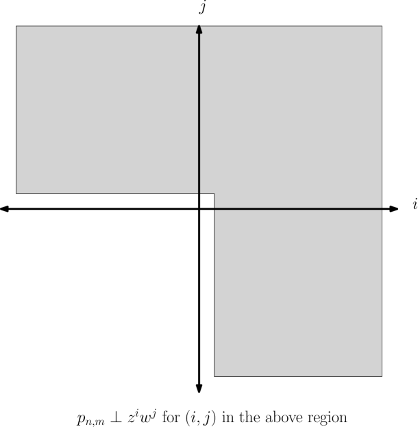
Figure 1. Orthogonalities of $p_{n,m}$

Write $p_{n,m}(z,w)=\sum^{m}_{i=0}p_{i}(z)w^{i}$.

Since $p_{n,m}(z,w)$ is stable it follows from the Schur-Cohn test for stability [1] that the $m\times m$ matrix

$$T_{m}(z) =\begin{bmatrix}p_{0}(z)&&\bigcirc\\ p_{1}(z)&\ddots\\ \vdots\\ p_{m-1}(z)&\cdots&p_{0}(z)\end{bmatrix}\begin{bmatrix}\bar{p}_{0}(1/z)&\bar{p}_{1}(1/z)&\cdots&\bar{p}_{m-1}(1/z)\\ &\ddots\\ \bigcirc&\cdots&\cdots&\bar{p}_{0}(1/z)\end{bmatrix}$$

$$\qquad-\begin{bmatrix}\bar{p}_{m}(1/z)&&\bigcirc\\ \vdots&\ddots\\ \bar{p}_{1}(1/z)&\cdots&\bar{p}_{m}(1/z)\end{bmatrix}\begin{bmatrix}p_{m}(z)&\cdots&p_{1}(z)\\ \vdots&\ddots\\ \bigcirc&&p_{m}(z)\end{bmatrix}$$ (2.1)

is positive definite for $|z|=1$. Here $\bar{p}_{j}(z)=\overline{p_{j}(\bar{z})}$.

Define the following parametrized version of a one variable Christoffel-Darboux kernel

$$L(z,w;\eta) =z^{n}\frac{p_{n,m}(z,w)\overline{p_{n,m}(1/\bar{z},\eta)}-\accentset{\leftarrow}{p}_{n,m}(z,w)\overline{\accentset{\leftarrow}{p}_{n,m}(1/\bar{z},\eta)}}{1-w\bar{\eta}}$$ (2.2)

$$=z^{n}[1,\ldots,w^{m-1}]T_{m}(z)[1,\ldots,\eta^{m-1}]^{{\dagger}}$$

$$=\sum_{j=0}^{m-1}a_{j}(z,w)\bar{\eta}^{j},$$

where $a_{j}(z,w),\ j=0,\ldots,m-1$ are polynomials in $(z,w)$, as the following lemma shows in addition to several other important observations.

Lemma 2.2.

Let $p_{n,m}(z,w)$ be a stable polynomial of degree $(n,m)$. Then,

1. $L$ is a polynomial of degree $(2n,m-1)$ in $(z,w)$ and a polynomial of degree $m-1$ in $\bar{\eta}$.

2. $L(\cdot,\cdot;\eta)$ spans a subspace of dimension $m$ as $\eta$ varies over $\mathbb{C}$.

3. $L$ is symmetric in the sense that

   $$L(z,w;\eta)=z^{2n}(w\bar{\eta})^{m-1}\overline{L(1/\bar{z},1/\bar{w};1/\bar{\eta})},$$

   so $a_{k}=\accentset{\leftarrow}{a}_{m-k-1}$.

4. $L$ can be written as

   $$L(z,w;\eta)=p_{n,m}(z,w)A(z,w;\eta)+\accentset{\leftarrow}{p}_{n,m}(z,w)B(z,w;\eta)$$

   where $A,B$ are polynomials of degree $(n,m-1,m-1)$ in $(z,w,\bar{\eta})$.

Proof.

The numerator of $L$ vanishes when $w=1/\bar{\eta}$, so the factor $(1-w\bar{\eta})$ divides the numerator. This gives (1).

For (2), when $|z|=1$ use equation (2.2). Since $T_{m}(z)>0$ for $|z|=1$, $L(z,w;\eta)$ spans a set of polynomials of dimension $m$.

For (3), this is just a computation.

For (4), observe that (suppressing the dependence of $p$ on $n$ and $m$),

$$z^{n}\frac{p(z,w)\overline{p(1/\bar{z},\eta)}-\accentset{\leftarrow}{p}(z,w)\overline{\accentset{\leftarrow}{p}(1/\bar{z},\eta)}}{1-w\bar{\eta}}$$

$$=p(z,w)\underset{A(z,w;\eta)}{\underbrace{\left(\frac{\bar{\eta}^{m}\accentset{\leftarrow}{p}(z,1/\bar{\eta})-\bar{\eta}^{m}\accentset{\leftarrow}{p}(z,w)}{1-w\bar{\eta}}\right)}}+\accentset{\leftarrow}{p}(z,w)\underset{B(z,w;\eta)}{\underbrace{\left(\frac{\bar{\eta}^{m}p(z,w)-\bar{\eta}^{m}p(z,1/\bar{\eta})}{1-w\bar{\eta}}\right)}}.$$ (2.3)

∎

3. Orthogonality relations in $L^{2}(1/|p_{n,m}|^{2}d\sigma)$

Our main goal is to prove that $L$ and $a_{0},\dots,a_{m-1}$ possess a great many orthogonality relations in $L^{2}(1/|p_{n,m}|^{2}d\sigma)$. The orthogonality relations of $L$ are depicted in Figure 2.

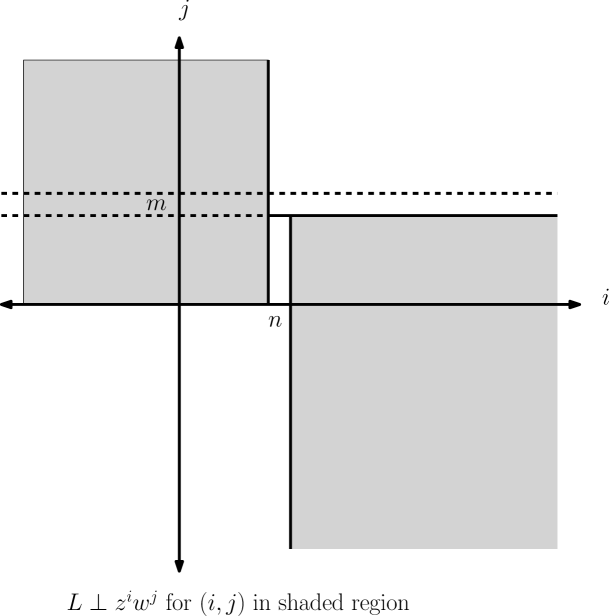
Figure 2. Orthogonalities of $L$. See Theorem 3.1

Theorem 3.1.

In $L^{2}(1/|p_{n,m}|^{2}d\sigma)$, each $a_{k}$ is orthogonal to the set

$$\mathcal{O}_{k}= \{z^{i}w^{j}:i>n,j<0\}$$

$$\cup\{z^{i}w^{j}:0\leq j<m,j\neq k\}$$

$$\cup\{z^{i}w^{j}:i<n,j\geq m\}$$

$$\cup\{z^{i}w^{k}:i\neq n\}.$$

In $L^{2}(1/|p_{n,m}|^{2}d\sigma)$, $L(\cdot,\cdot;\eta)$ is orthogonal to the set

$$\mathcal{O}= \{z^{i}w^{j}:i>n,j<0\}$$

$$\cup\{z^{i}w^{j}:i\neq n,0\leq j<m\}$$ (3.1)

$$\cup\{z^{i}w^{j}:i<n,j\geq m\}.$$

Note that

$$\mathcal{O}_{k} =\{z^{n}w^{j}:0\leq j<m,j\neq k\}\cup\mathcal{O},$$

$$\mathcal{O} =\bigcap_{k=0}^{m-1}\mathcal{O}_{k}.$$

Corollary 3.2.

In $L^{2}(1/|p_{n,m}|^{2}d\sigma)$, the polynomial $a_{k}$ is uniquely determined (up to unimodular multiples) by the conditions:

$$a_{k}\in\mathrm{span}\{z^{i}w^{j}:(0,0)\leq(i,j)\leq(2n,m-1)\},$$

$$a_{k}\perp \{z^{i}w^{j}:(0,0)\leq(i,j)\leq(2n,m-1),j\neq k\}$$

$$\cup\{z^{i}w^{k}:0\leq i\leq 2n,i\neq n\},$$

and

$$||a_{k}||^{2}=\int_{-\pi}^{\pi}T_{k,k}(e^{i\theta},e^{i\theta})\frac{d\theta}{2\pi}.$$

(The last fact follows from Proposition 6.1, which is not currently essential.)

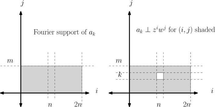
Figure 3. The $a_{k}$ are uniquely determined by the above properties. See Corollary 3.2.

Remark 3.3.

We emphasize that (1) each $a_{k}$ is explicitly given from coefficients of $p_{n,m}$, (2) each $a_{k}$ is determined by the orthogonality relations in Corollary 3.2 (depicted in Figure 3), and (3) each satisfies the additional orthogonality relations from Theorem 3.1. One useful consequence of this is that the set

$$\{z^{j}a_{k}(z,w):j\in\mathbb{Z},0\leq k<m\}$$

is dual to the monomials

$$\{z^{j+n}w^{k}:j\in\mathbb{Z},0\leq k<m\}$$

within in the subspace

$$S=\overline{\mathrm{span}}\{z^{j}w^{k}:j\in\mathbb{Z},0\leq k<m\}.$$

Namely,

$$\langle z^{j_{1}+n}w^{k_{1}},z^{j_{2}}a_{k_{2}}\rangle=0$$

unless $j_{1}=j_{2}$ and $k_{1}=k_{2}$.

In particular, if $f\in S$, then

$$f\perp z^{j}a_{k}\text{ implies }\hat{f}(j+n,k)=0.$$ (3.2)

4. The proof of Theorem 3.1

We begin by writing

$$A(z,w;\eta)=\sum_{j=0}^{m-1}A_{j}(z,w)\bar{\eta}^{j}\qquad B(z,w;\eta)=\sum_{j=0}^{m-1}B_{j}(z,w)\bar{\eta}^{j}.$$

Recall equation (2.2) and Lemma 2.2 item (4). By examining coefficients of $\bar{\eta}^{j}$ in $L$

$$a_{j}=p_{n,m}A_{j}+\accentset{\leftarrow}{p}_{n,m}B_{j}.$$

Also, $A_{j}$ and $B_{j}$ have at most degree $j$ in $w$. To see this, recall equation (2.3) and observe that

$$A(z,w;\eta)=\sum_{j}\accentset{\leftarrow}{p}_{j}(z)\bar{\eta}^{j}\frac{1-(w\bar{\eta})^{m-j}}{1-w\bar{\eta}}$$

which shows that $A_{j}(z,w)$ has degree at most $j$ in $w$ (i.e. powers of $w$ only occur next to greater powers of $\eta$). The same holds for $B$.

Proof of Theorem 3.1.

By Lemma 2.1, $p_{n,m}$ is orthogonal to

$$\{z^{i}w^{j}:(i,j)\nleq(0,0)\}$$

and since $A_{k}$ has degree at most $n$ in $z$ and $k$ in $w$,

$$p_{n,m}A_{k}\text{ is orthogonal to }\{z^{i}w^{j}:(i,j)\nleq(n,k)\}.$$

Also,

$$\accentset{\leftarrow}{p}_{n,m}B_{k}\text{ is orthogonal to }\{z^{i}w^{j}:(i,j)\ngeq(n,m)\}$$

since the orthogonality relation for $\accentset{\leftarrow}{p}_{n,m}$ (also from Lemma 2.1) is unaffected by multiplication by holomorphic monomials.

Hence, $a_{k}=p_{n,m}A_{k}+\accentset{\leftarrow}{p}_{n,m}B_{k}$ is orthogonal to the intersection of these sets; namely,

$$\{z^{i}w^{j}:(i,j)\nleq(n,k)\text{ and }(i,j)\ngeq(n,m)\}.$$ (4.1)

Since

$$a_{m-k-1}\perp\{z^{i}w^{j}:(i,j)\nleq(n,m-k-1)\text{ and }(i,j)\ngeq(n,m)\}$$

and since $a_{k}=\accentset{\leftarrow}{a}_{m-k-1}=z^{2n}w^{m-1}\overline{a_{m-k-1}(1/\bar{z},1/\bar{w})}$,

$$a_{k}\perp \{z^{2n-i}w^{m-j-1}:(i,j)\nleq(n,m-k-1)\text{ and }(i,j)\ngeq(n,m)\}$$

$$=\{z^{i}w^{j}:(n,k)\nleq(i,j)\text{ and }(n,-1)\ngeq(i,j)\}.$$ (4.2)

Hence, $a_{k}$ is orthogonal to the union of the sets in (4.1) and (4.2). The set in (4.2) contains $\{z^{i}w^{j}:i<n,j\geq 0\}$ and the set in (4.1) contains $\{z^{i}w^{j}:i>n,j\leq m-1\}$. Also, the set in (4.1) contains $\{z^{n}w^{j}:k<j\leq m-1\}$ while the set in (4.2) contains $\{z^{n}w^{j}:0\leq j<k\}$. Combining all of this we get $a_{k}\perp\mathcal{O}_{k}$.

Finally, $L$ is orthogonal to the intersection of $\mathcal{O}_{0},\dots,\mathcal{O}_{m-1}$. ∎

We now look at the space generated by shifting the $a_{k}$’s by powers of $z$.

Theorem 4.1.

With respect to $L^{2}(\frac{d\sigma}{|p_{n,m}|^{2}})$,

$$\overline{\mathrm{span}}\{z^{i}a_{j}(z,w):0\leq i,0\leq j<m\}$$

$$=\overline{\mathrm{span}}\{z^{i}w^{j}:0\leq i,0\leq j<m\}\ominus\overline{\mathrm{span}}\{z^{i}w^{j}:0\leq i<n,0\leq j<m\}$$ (4.3)

and this is orthogonal to the larger set

$$\overline{\mathrm{span}}\{z^{i}w^{j}:i<n,j\geq 0\}.$$

Proof.

Since the $a_{k}$ are polynomials of degree at most $m-1$ in $w$, it is clear that

$$\overline{\mathrm{span}}\{z^{i}a_{j}(z,w):0\leq i,0\leq j<m\}\subset\overline{\mathrm{span}}\{z^{i}w^{j}:0\leq i,0\leq j<m\}.$$

By Theorem 3.1, the $a_{k}$ are orthogonal to the spaces

$$\overline{\mathrm{span}}\{z^{i}w^{j}:i<n,j\geq 0\}\supset\overline{\mathrm{span}}\{z^{i}w^{j}:i<n,0\leq j<m\},$$

and since these spaces are invariant under multiplication by $\bar{z}$, the polynomials $z^{i}a_{k}$ are also orthogonal to these spaces for all $i\geq 0$. So,

$$\overline{\mathrm{span}}\{z^{i}a_{j}(z,w):0\leq i,0\leq j<m\}\perp\overline{\mathrm{span}}\{z^{i}w^{j}:i<n,j\geq 0\}.$$

Therefore,

$$\overline{\mathrm{span}}\{z^{k}a_{j}(z,w):0\leq k,0\leq j<m\}$$

$$\subset\overline{\mathrm{span}}\{z^{i}w^{j}:0\leq i,0\leq j<m\}\ominus\overline{\mathrm{span}}\{z^{i}w^{j}:0\leq i<n,0\leq j<m\}$$ (4.4)

and this containment must in fact be an equality.

Indeed, any $f$ in

$$\overline{\mathrm{span}}\{z^{i}w^{j}:0\leq i,0\leq j<m\}$$

which is orthogonal to $\{z^{k}a_{j}(z,w):0\leq k,0\leq j<m\}$ satisfies $\hat{f}(i,j)=0$ for $i\geq n$ and $0\leq j<m$ by Remark 3.3 and equation (3.2). Such an $f$ cannot also be orthogonal to the space $\overline{\mathrm{span}}\{z^{i}w^{j}:0\leq i<n,0\leq j<m\}$ without being identically zero. ∎

Define

$$H= \mathrm{span}\{z^{i}w^{j}:(0,0)\leq(i,j)\leq(n,m-1)\}$$

$$\ominus\mathrm{span}\{z^{i}w^{j}:(0,0)\leq(i,j)\leq(n-1,m-1)\}.$$

Define also the reflection $\accentset{\leftarrow}{H}$

$$\accentset{\leftarrow}{H}= \mathrm{span}\{z^{i}w^{j}:(0,0)\leq(i,j)\leq(n,m-1)\}$$

$$\ominus\mathrm{span}\{z^{i}w^{j}:(1,0)\leq(i,j)\leq(n,m-1)\}.$$

Proposition 4.2.

We have the following orthogonal direct sum decompositions in $L^{2}(1/|p_{n,m}|^{2}d\sigma)$

$$\overline{\mathrm{span}}\{z^{k}a_{j}(z,w):0\leq k,0\leq j<m\}=\bigoplus_{i=0}^{\infty}z^{i}H$$ (4.5)

$$\mathcal{H}_{1}:=\overline{\mathrm{span}}\{z^{k}w^{j}:0\leq k,0\leq j<m\}=\bigoplus_{i=0}^{\infty}z^{i}\accentset{\leftarrow}{H}.$$ (4.6)

If $K_{H}$ is the reproducing kernel for $H$ and $K_{\accentset{\leftarrow}{H}}$ is the reproducing kernel for $\accentset{\leftarrow}{H}$, then the reproducing kernel for the spaces in (4.5) and (4.6) are given by

$$\frac{K_{H}(z,w;z_{1},w_{1})}{1-z\bar{z}_{1}}\text{ and }\frac{K_{\accentset{\leftarrow}{H}}(z,w;z_{1},w_{1})}{1-z\bar{z}_{1}}$$

respectively.

Proof.

Now $H$ is an $m$ dimensional space of polynomials contained in the space (4.3) of the previous theorem. In particular,

$$H\perp\overline{\mathrm{span}}\{z^{i}w^{j}:i<n,j\geq 0\},$$ (4.7)

and

$$H=\overline{\mathrm{span}}\{z^{i}w^{j}:i\leq n,0\leq j<m\}\ominus\overline{\mathrm{span}}\{z^{i}w^{j}:i<n,0\leq j<m\}$$

since this space is also $m$ dimensional and contains $H$. From this it is clear that $H\perp z^{i}H$ for $i>0$ and we have

$$\bigoplus_{i=0}^{\infty}z^{i}H= \overline{\mathrm{span}}\{z^{i}w^{j}:0\leq j<m\}$$

$$\ominus\overline{\mathrm{span}}\{z^{i}w^{j}:i<n,0\leq j<m\}.$$

Since shifts of $H$ are contained in $\overline{\mathrm{span}}\{z^{i}w^{j}:0\leq i,0\leq j<m\}$, we must have

$$\bigoplus_{i=0}^{\infty}z^{i}H= \overline{\mathrm{span}}\{z^{i}w^{j}:0\leq i,0\leq j<m\}$$

$$\ominus\overline{\mathrm{span}}\{z^{i}w^{j}:0\leq i<n,0\leq j<m\}$$

which combined with (4.3) gives (4.5).

Next, $\accentset{\leftarrow}{H}$ is also $m$ dimensional and by (4.7) is orthogonal to

$$\{z^{i}w^{j}:i>0;j<m\}$$

which in particular contains the strip $\{z^{i}w^{j}:i>0;0\leq j<m\}=z\{z^{i}w^{j}:i\geq 0;0\leq j<m\}$. So,

$$\accentset{\leftarrow}{H}= \overline{\mathrm{span}}\{z^{i}w^{j}:0\leq i,0\leq j<m\}$$

$$\ominus z\ \overline{\mathrm{span}}\{z^{i}w^{j}:0\leq i,0\leq j<m\}$$

by dimensional considerations. Therefore,

$$\mathcal{H}_{1}=\bigoplus_{j\geq 0}z^{j}\accentset{\leftarrow}{H}.$$

The formulas for the reproducing kernels are direct consequences of the orthogonal decompositions (see [4] for more on this). ∎

Lemma 4.3.

In $L^{2}(1/|p_{n,m}|^{2}d\sigma)$ the reproducing kernel for

$$\mathcal{H}=\overline{\mathrm{span}}\{z^{i}w^{j}:(0,0)\leq(i,j)\ngeq(n,m)\}$$

is

$$\frac{p_{n,m}(z,w)\overline{p_{n,m}(z_{1},w_{1})}-\overleftarrow{p_{n,m}}(z,w)\overline{\overleftarrow{p_{n,m}}(z_{1},w_{1})}}{(1-z\bar{z}_{1})(1-w\bar{w}_{1})}.$$

Proof.

First,

$$K(z,w;z_{1},w_{1})=K_{(z_{1},w_{1})}(z,w)=\frac{p_{n,m}(z,w)\overline{p_{n,m}(z_{1},w_{1})}}{(1-z\bar{z}_{1})(1-w\bar{w}_{1})}$$

is the reproducing kernel for $\overline{\mathrm{span}}\{z^{i}w^{j}:(0,0)\leq(i,j)\}$ since

$$\langle f,K_{(z_{1},w_{1})}\rangle =\int_{\mathbb{T}^{2}}\frac{f(z,w)}{p_{n,m}(z,w)}p_{n,m}(z_{1},w_{1})\frac{dzdw}{(2\pi i)^{2}zw(1-\bar{z}z_{1})(1-\bar{w}w_{1})}$$

$$=\frac{f(z_{1},w_{1})}{p_{n,m}(z_{1},w_{1})}p_{n,m}(z_{1},w_{1})=f(z_{1},w_{1})$$

by the Cauchy integral formula. On the other hand,

$$\frac{\accentset{\leftarrow}{p}_{n,m}(z,w)\overline{\overleftarrow{p_{n,m}}(z_{1},w_{1})}}{(1-z\bar{z}_{1})(1-w\bar{w}_{1})}$$ (4.8)

is the reproducing kernel for

$$\overline{\mathrm{span}}\{z^{i}w^{j}:(0,0)\leq(i,j)\}\ominus\mathcal{H}.$$ (4.9)

To see this it is enough to show that $\{z^{i}w^{j}\accentset{\leftarrow}{p}_{n,m}:(0,0)\leq(i,j)\}$ is an orthonormal basis for the space (4.9). By Lemma 2.1, $z^{i}w^{j}\accentset{\leftarrow}{p}_{n,m}$ is in the space in (4.9) for every $i,j\geq 0$ and it is easy to check that these polynomials form an orthonormal set. We show that their span is dense.

We may write $\accentset{\leftarrow}{p}_{n,m}=cz^{n}w^{m}+\text{lower order terms}$ with $c\neq 0$, since $p_{n,m}$ is stable. Now, let $f$ be in the space in (4.9). If $f\perp\accentset{\leftarrow}{p}_{n,m}=cz^{n}w^{m}+\text{lower order terms}$, then since $f$ is already orthogonal to the “lower order terms” we see that $f\perp z^{n}w^{m}$. Inductively, then, we see that assuming $f\perp z^{i}w^{j}$ for all $i\leq N$ and $j\leq M$ but $(i,j)\neq(N,M)$ and assuming $f\perp z^{N}w^{M}\accentset{\leftarrow}{p}_{n,m}$, we automatically get $f\perp z^{N}w^{M}$ since $f$ will be orthogonal to the lower order terms in $z^{N}w^{M}\accentset{\leftarrow}{p}_{n,m}$. Therefore, if $f$ in (4.9) is orthogonal to $\{z^{i}w^{j}\accentset{\leftarrow}{p}_{n,m}:i,j\geq 0\}$ there can be no minimal $(i,j)\geq(n,m)$ (in the partial order on pairs) such that $f$ is not orthogonal to $z^{i}w^{j}$. In particular, $f\perp z^{i}w^{j}$ for all $i\geq n$ and $j\geq m$ and by (4.9) $f\perp\mathcal{H}$, which forces $f\equiv 0$.

So, $\{z^{i}w^{j}\accentset{\leftarrow}{p}_{n,m}:(0,0)\leq(i,j)\}$ is an orthonormal basis for the space in (4.9) while (4.8) is the reproducing kernel for this space.

Finally, the reproducing kernel for

$$\mathcal{H}=\overline{\mathrm{span}}\{z^{i}w^{j}:(0,0)\leq(i,j)\}\ominus(\overline{\mathrm{span}}\{z^{i}w^{j}:(0,0)\leq(i,j)\}\ominus\mathcal{H})$$

is the difference of the reproducing kernels we have just calculated. Namely,

$$\frac{p_{n,m}(z,w)\overline{p_{n,m}(z_{1},w_{1})}-\overleftarrow{p_{n,m}}(z,w)\overline{\overleftarrow{p_{n,m}}(z_{1},w_{1})}}{(1-z\bar{z}_{1})(1-w\bar{w}_{1})}.$$

∎

5. The bivariate Christoffel-Darboux formula

Set

$$H_{1}= \mathrm{span}\{z^{i}w^{j}:0\leq i\leq n,0\leq j\leq m-1\}$$

$$\ominus\mathrm{span}\{z^{i}w^{j}:0\leq i\leq n-1,0\leq j\leq m-1\}$$

and

$$\accentset{\leftarrow}{H}_{2}= \mathrm{span}\{z^{i}w^{j}:0\leq i\leq n-1,0\leq j\leq m\}$$

$$\ominus\mathrm{span}\{z^{i}w^{j},0\leq i\leq n-1,1\leq j\leq m\}.$$

The two variable Christoffel-Darboux formula is the following.

Theorem 5.1.

Let $p_{n,m}$ be a stable polynomial. Let $K_{1}$ be the reproducing kernel for $H_{1}$ and let $K_{2}$ be the reproducing kernel for $\accentset{\leftarrow}{H}_{2}$. Then

$$p_{n,m}(z,w)\overline{p_{n,m}(z_{1},w_{1})}-\overleftarrow{p_{n,m}}(z,w)\overline{\overleftarrow{p_{n,m}}(z_{1},w_{1})}$$

$$=(1-w\bar{w}_{1})K_{1}(z,w;z_{1},w_{1})+(1-z\bar{z}_{1})K_{2}(z,w;z_{1},w_{1}),$$

Proof.

Set

$$\mathcal{H} =\overline{\mathrm{span}}\{z^{i}w^{j}:(0,0)\leq(i,j)\ngeq(n,m)\}$$

$$\mathcal{H}_{1} =\overline{\mathrm{span}}\{z^{i}w^{j}:0\leq i,0\leq j<m\}$$

$$\mathcal{H}_{2} =\overline{\mathrm{span}}\{z^{i}w^{j}:0\leq i<n,0\leq j\}$$

and notice that $\mathcal{H}_{1}$ and $\mathcal{H}_{2}$ together span $\mathcal{H}$.

Theorem 4.1 says

$$\overline{\mathrm{span}}\{z^{i}a_{j}(z,w):0\leq i,0\leq j<m\}$$ (5.1)

$$=\mathcal{H}_{1}\ominus(\mathcal{H}_{1}\cap\mathcal{H}_{2})\subset\mathcal{H}\ominus\mathcal{H}_{2}$$ (5.2)

which a fortiori implies

$$\mathcal{H}_{1}\ominus(\mathcal{H}_{1}\cap\mathcal{H}_{2})=\mathcal{H}\ominus\mathcal{H}_{2}.$$

To see this, suppose $f\in(\mathcal{H}\ominus\mathcal{H}_{2})\ominus(\mathcal{H}_{1}\ominus(\mathcal{H}_{1}\cap\mathcal{H}_{2}))$. Then, $f\in\mathcal{H}\ominus\mathcal{H}_{1}$. As $\mathcal{H}_{1}$ and $\mathcal{H}_{2}$ span $\mathcal{H}$, such an $f$ must be orthogonal to all of $\mathcal{H}$ and must equal $0$.

The reproducing kernel for the space

$$\mathcal{H}\ominus\mathcal{H}_{2}=\bigoplus_{j\geq 0}z^{j}H_{1}\text{ is }\frac{K_{1}(z,w;z_{1},w_{1})}{1-z\bar{z}_{1}}$$

from Proposition 4.2.

If we interchange the roles of $z$ and $w$ in Proposition 4.2 we see that

$$\frac{K_{2}(z,w;z_{1},w_{1})}{1-w\bar{w}_{1}}$$

is the reproducing kernel for $\mathcal{H}_{2}$.

Finally, the reproducing kernel for $\mathcal{H}=\mathcal{H}_{2}\oplus(\mathcal{H}\ominus\mathcal{H}_{2})$ can be written in two ways. On the one hand it equals

$$\frac{p_{n,m}(z,w)\overline{p_{n,m}(z_{1},w_{1})}-\overleftarrow{p_{n,m}}(z,w)\overline{\overleftarrow{p_{n,m}}(z_{1},w_{1})}}{(1-z\bar{z}_{1})(1-w\bar{w}_{1})},$$

but on the other it equals

$$\frac{K_{2}(z,w;z_{1},w_{1})}{1-w\bar{w}_{1}}+\frac{K_{1}(z,w;z_{1},w_{1})}{1-z\bar{z}_{1}}$$

by the discussion above. Equating these formulas and multiplying through by $(1-z\bar{z}_{1})(1-w\bar{w}_{1})$, yields the desired formula. ∎

6. Parametric orthogonal polynomials

The above results also shed light on the parametric orthogonal polynomials. The following proposition shows that the inner products of $a_{0},\dots,a_{m-1}$ with respect to $L^{2}(d\mu^{\theta},\mathbb{T})$ for the measures parametrized by $z=e^{i\theta}\in\mathbb{T}$

$$d\mu^{\theta}(w)=\frac{|dw|}{2\pi|p_{n,m}(e^{i\theta},w)|^{2}}$$ (6.1)

are trigonometric polynomials in $z$.

Proposition 6.1.

For fixed $z\in\mathbb{T}$

$$\int_{\mathbb{T}}|L(z,w;\eta)|^{2}\frac{|dw|}{2\pi|p_{n,m}(z,w)|^{2}}=\bar{z}^{n}L(z,\eta;\eta)$$ (6.2)

and as a consequence

$$\int_{\mathbb{T}}\overline{a_{i}(z,w)}a_{j}(z,w)\frac{|dw|}{2\pi|p_{n,m}(z,w)|^{2}}=T_{i,j}(z).$$ (6.3)

Proof.

For $z\in\mathbb{T}$ the expression

$$\bar{z}^{n}L(z,w;\eta)=\frac{p_{n,m}(z,w)\overline{p_{n,m}(z,\eta)}-\accentset{\leftarrow}{p}_{n,m}(z,w)\overline{\accentset{\leftarrow}{p}_{n,m}(z,\eta)}}{1-w\bar{\eta}}$$

is the reproducing kernel/Christoffel-Darboux kernel for polynomials in $w$ of degree at most $m-1$ with respect to the measure $|dw|/(2\pi|p_{n,m}(z,w)|^{2})$. Indeed, this is one of the main consequences of the Christoffel-Darboux formula in one variable (see [7] equation (34) or [8] Theorem 2.2.7). It is a general fact about reproducing kernels $K(w,\eta)=K_{\eta}(w)$ that

$$||K(\cdot,\eta)||^{2}=\langle K_{\eta},K_{\eta}\rangle=K(\eta,\eta).$$

Using these two observations, (6.2) follows. Equation (6.3) follows from matching the coefficients of $\eta^{i}\bar{\eta}^{j}$ in (6.2). ∎

Given $T_{m}(z)$ defined in equation (2), set $D_{i}(\theta)$ as the determinant of the $i\times i$ submatrix of $T_{m}(e^{i\theta})$ obtained by keeping the first $i$ rows and columns and set $D_{0}=1$ . We now perform the LU decomposition of $T_{m}$ which because it is positive definite does not require any pivoting. Set

$$[\phi^{\theta}_{m-1}(w),\ldots,\phi^{\theta}_{0}(w)]^{T}=U(\theta)[w^{m-1},\ldots,1]^{T},$$ (6.4)

where $U(\theta)$ is the upper triangular factor obtained from the LU decomposition of $T_{m}$ without pivoting. We find:

Proposition 6.2.

Suppose $p_{n,m}$ is a stable polynomial then $\{\phi^{\theta}_{i}(w)\}_{i=0}^{m-1}$ satisfy the relations

• $\phi^{\theta}_{i}(w)$ is a polynomial in $w$ of degree $i$ with leading coefficient, $\frac{D_{m-i}(\theta)}{D_{m-i+1}(\theta)}$,

• $\int_{\mathbb{T}}\phi^{\theta}_{i}(w)\overline{\phi^{\theta}_{j}(w)}d\mu^{\theta}(w)=\delta_{i,j}\frac{D_{m-i}(\theta)}{D_{m-i+1}(\theta)}$,

which uniquely specify the polynomials. The above implies

$$\int_{[0,2\pi]^{2}}e^{i\theta k}D_{m-j+1}(\theta)\phi^{\theta}_{j}(e^{i\phi})\overline{\phi^{\theta}_{j}(e^{i\phi})}\frac{d\theta d\phi}{(2\pi)^{2}|p_{n,m}(e^{i\theta},e^{i\phi})|^{2}}=0,\ k>n(m-j).$$

Proof.

From the definition of $T_{m}$ we see that it is the inverse of the $m\times m$ moment matrix associated with $d\mu^{\theta}(w)$. The first part of the result now follows from the one dimensional theory of polynomials orthogonal on the unit circle. The second part follows since $z^{n(m-j)}D_{m-j}(\theta)$ is polynomial in $z$. ∎

References

- [1] J. S. Geronimo and H. J. Woerdeman, Positive extensions, Fejér-Riesz factorization and autoregressive filters in two variables, Annals of Math 160 (2004), 839–906.
- [2] J. S. Geronimo and H. J. Woerdeman,Two variable orthogonal polynomials on the bicircle and structured matrices, SIAM J Matrix Anal. Appl 29 (2007) 796–825.
- [3] A. Grinshpan, D. S. Kaliuzhnyi-Verbovetskyi, V. Vinnikov, and H. J. Woerdeman, Classes of tuples of commuting contractions satisfying the multivariable von Neumann inequality, J. Funct. Anal. 57 (2009), 3035–3054.
- [4] G. Knese, Bernstein-Szegő measures on the two dimensional torus, Indiana Univ. Math. J. 57 (2008), 1353–1376.
- [5] G. Knese, Polynomials with no zeros on the bidisk, Anal. PDE 3 (2010), 109–149.
- [6] G. Knese, Kernel decompositions for Schur functions on the polydisk, Complex Analysis and Operator Theory (2010), to appear.
- [7] H. Landua, Maximum entropy and the moment problem, Bull. Amer. Math. Soc. (N.S.) 16 (1987), no. 1, 47–77.
- [8] B. Simon, Orthogonal polynomials on the unit circle. Part 1., Classical theory. American Mathematical Society Colloquium Publications 54, Part 1. American Mathematical Society, Providence, RI, 2005.
- [9] H. J. Woerdeman, A general Christoffel-Darboux type formula, Integral Equations Operator Theory 67 (2010), 203–213.