Classical Helium Atom with Radiation Reaction

Abstract

We study a classical model of Helium atom in which, in addition to the Coulomb forces, the radiation reaction forces are taken into account. This modification brings in the model a new qualitative feature of a global character. Indeed, as pointed out by Dirac, in any model of classical electrodynamics of point particles involving radiation reaction one has to eliminate, from the a priori conceivable solutions of the problem, those corresponding to the emission of an infinite amount of energy. We show that the Dirac prescription solves a problem of inconsistency plaguing all available models which neglect radiation reaction, namely, the fact that in all such models most initial data lead to a spontaneous breakdown of the atom. A further modification is that the system thus acquires a peculiar form of dissipation. In particular, this makes attractive an invariant manifold of special physical interest, the zero–dipole manifold, that corresponds to motions in which no energy is radiated away (in the dipole approximation). We finally study numerically the invariant measure naturally induced by the time–evolution on such a manifold, and this corresponds to studying the formation process of the atom. Indications are given that such a measure may be singular with respect to that of Lebesgue.

At variance with the existing works on the dynamical properties of classical atomic systems (see for example Refs. nich, ; bohr, ; lang, ; kaneko1, ; kaneko2, ; poir, ; jayme, ; jayme2, ), in this paper we take into account, for the case of the Helium atom, the effects on the dynamics due to the radiation emitted by the electrons during their motion. This introduces a qualitative change in the dynamics, with respect to the purely Coulomb model, because the model now corresponds to a non conservative dynamical system. This leads to the appearing of an “attractive” manifold of stable periodics orbits, where attractive is to be understood in a proper sense which will be explained below. The aim of this paper is to study the properties of such a manifold, through analytical and numerical methods.

I Introduction

The studies on the dynamical properties of classical atomic models, in which only Coulomb forces are taken into account, have a long history, going back to Nicholson, Bohr and Langmuir (see Refs. nich, ; bohr, ; lang, ). The main result found in such old works (see the work nich, of Nicholson for the case of Beryllium, at those times called Nebulium) is that there exist periodic orbits having “normal mode frequencies” whose ratios are near to those of the observed spectral lines. Among the recent works on this subject a particularly relevant place is taken by the papers of De Luca jayme ; jayme2 on the Helium atom. This author went beyond the Coulomb approximation, taking retardation of the electromagnetic forces into account. This was obtained through a perturbation scheme which, truncated in a suitable way, leads to the conservative Darwin lagrangian that one finds illustrated in common textbookslandau ; jackson . In such a way the scale invariance of the purely Coulomb model was eliminated, and the result of Nicholson could be improved, showing that for the Helium atom there exist periodic orbits leading to dynamical frequencies which themselves, and not only their ratios, have a rather good agreement with the empirical spectral frequencies.

On the other hand, it was known since the time of Nicholson, and confirmed for example by Poirier poir , that all such periodic orbits are unstable. More recently Yamamoto and Kanekokaneko1 ; kaneko2 showed, for the case of Helium, that the instability of the periodic orbits actually corresponds to a much more general and acute form of instability. Indeed they found that the vast majority of initial data with negative energy lead to the autoionization of the atom, namely, to motions in which one of the electrons is expelled. One can see that this occurs also for a generic atom, and even in a stronger way, inasmuch as one meets with motions in which all electrons but one are expelled. So, the whole classical theory of atomic models seems to be plagued by a general failure, for which no remedy is known.

One usually takes the pragmatic attitude of just forgetting the autoionizing motions. One should however indicate an internal dynamical justification of a more general character for such a selection of the initial data. Moreover, one might hope that such a general prescription would also automatically explain why the system chooses to fall (through some peculiar kind of dissipation) on the physically interesting periodic orbits, for which an agreement betweeen dynamical and spectral frequencies is found. Obviously, satisfying the latter point requires to abandon a purely lagrangian, and thus conservative, approach to the problem, by taking electromagnetic radiation into account.

This is precisely what we do in the present paper, where we take into account the emission of radiation due to the accelerations of the electrons in the simplest possible way, namely, by adding to the Coulomb forces the radiation reaction ones. So, in a sense our model is complementary to that of De Luca, who introduces only the conservative terms produced by the Darwin approximation scheme, and neglects dissipation. We leave for future work the study of a model which takes both features into account.

It will be shown here that the modification of the Coulomb model that takes radiation into account, in the first place gives a model in which the autoionization problem no more arises. This is due to the fact, first pointed out by Dirac in the general context of classical electrodynamics of point particlesdirac , that most initial data in the phase space suited to the model lead to motions in which an infinite amount of energy is emitted, so that the definition of the model has to be complemented by the explicit prescription that such initial data have to be discarded. The remaining initial data (constituting a set that will be called here the Dirac or physical manifold) will be shown to lead to motions in which the phenomenon of autoionization no more occurs. So, the elimination of the initial points in phase space leading to autoionizing solutions appears no more as a special trick to be strangely introduced ad hoc, but rather as a particular case of a completely general prescription that, following Dirac, has always to be introduced when dealing with classical models of matter–radiation interaction involving point particles.

Then we study the dynamics on the Dirac physical manifold, in which the Dirac precription turns out to introduce a dissipation af a peculiar type. We show that the Dirac prscription allows one to find (and in a easy way) all periodic orbits, proving furthermore that they form in phase space a manifold. This is just the zero–dipole manifold, which is constituted of phase–space points leading to motions that do not radiate energy away in the dipole approximation. A major aim of this paper is to study such a manifold. We first show that it is an attractor, for initial states with negative energy. Then we study, by numerical methods, the invariant measure naturally induced on it by the time–flow. This amounts to studying the formation process of the Helium atom, namely, motions having initial data with the two electrons coming from infinity that are then captured by the nucleus, and finally fall on the zero–dipole manifold, where emission of energy comes to an end.

From the point of view of the theory of dynamical systems, an interesting result we find is that, while the attractor (the zero–dipole manifold) is really simple as a manifold (being just a portion of a linear subspace in the system’s phase space), it is the invariant measure induced on it by the time evolution that is very peculiar. Indeed it is presumably singular with respect to the restriction of the Lebesgue measure, possibly having a fractal structure.

In Section 2 the model is introduced, and a preliminary analytical discussion of its properties is given. In Section 3 the numerical method for obtaining the invariant measure is described, and the numerical results are presented. The conclusions follow.

II The model

II.1 The radiation reaction for a single point–charge

Let us recall that, in the case of a single point–charge, the emission of radiation is taken into account without introducing the infinitely many degrees of freedom of the electromagnetic field, through the expedient of adding in the equation of motion for the particle an “effective force”. This force, which is traditionally called radiation reaction force and denoted by ${\mathbf{K}}^{rad}$, is given by

$${\mathbf{K}}^{rad}=\frac{2}{3}\frac{e^{2}}{c^{3}}\hskip 2.0pt\ddot{\hbox{}}\hskip 3.2pt\dot{\hbox{}}\kern-5.0pt{{\mathbf{x}}}\ ,$$ (1)

where $e$ is the charge of the particle, $c$ the speed of light, and ${{\mathbf{x}}}$ the position vector of the particle. The procedure which leads to such a force goes back to Planck, Lorentz and Abraham, and was given a final form in the work of Dirac dirac of the year 1938, in which an extension to the relativistic case was performed in an extremely elegant way. In its most elementary form, which is illustrated in standard textbooks (see Refs. landau, ; jackson, ; pauli, ; heitler, ), the procedure amounts to requiring that the effective force ${\mathbf{K}}^{rad}$ produces an energy loss consistent with the power radiated away by an accelerating particle according to the Larmor formula, namely, $(2/3)\,({e^{2}}/{c^{3}})\,|\ddot{{\mathbf{x}}}|^{2}$. As is well known, this force can also be interpreted as being produced by the regular part of the self–field of the particle, the divergent part having been reabsorbed through mass renormalization.

We illustrate now, in the simple case of the free particle in the nonrelativistic approximation, how the “runaway” solutions then show up. In terms of the particle’s acceleration ${\mathbf{a}}=\ddot{{\mathbf{x}}}$, the equation of motion for the free particle takes the form

$${\varepsilon}\dot{{\mathbf{a}}}={\mathbf{a}}\ ,$$

with

$${\varepsilon}=\frac{2}{3}\,\frac{e^{2}}{mc^{3}}$$ (2)

($m$ being the particle’s mass), with solutions ${\mathbf{a}}(t)={\mathbf{a}}_{0}\exp(t/{\varepsilon})$ depending parametrically on the initial acceleration ${\mathbf{a}}_{0}$. So, for generic initial data the solution exponentially explodes, i.e., presents runaway character, a fact which makes no sense for a free particle. Thus Dirac dirac introduces the explicit prescription that, for the case of a free particle, only the solutions with vanishing initial acceleration, ${\mathbf{a}}_{0}=0$, be retained. Now, the phase space $\mathcal{P}$ mathematically suited to the considered third–order equation of motion, is the vector space $\mathinner{\bf R}^{9}$, a point of which is defined by the coordinates $({\mathbf{x}},{\mathbf{v}},{\mathbf{a}})$ of position, velocity and acceleration. In such an ambient phase space $\mathcal{P}$, the physically meaningful phase space is thus the subset characterized by motions of nonrunaway type. This we will call “Dirac or physical manifold”, and coincides with the hyperplane ${\mathbf{a}}=0$.

More in general, in the presence of an external force vanishing at infinity, one should assume that for scattering states, in which the particle eventually behaves as a free one, the physical or nonrunaway manifold be defined by the asymptotic condition

$$\ddot{{\mathbf{x}}}(t)\to 0\quad\mathrm{for}\quad t\to+\infty\ .$$ (3)

Prescriptions of such a type may be formulated in a different way, which captures another side of the problem. One makes reference to the total energy emitted by the particle, namely, the quantity

$$\Delta E=m{\varepsilon}\int_{0}^{+\infty}|\ddot{{\mathbf{x}}}(t)|^{2}\,dt\ ,$$ (4)

and a physically natural requirement is then to restrict oneself to motions for which the amount of energy radiated away during the whole motion is finite, i.e., one has $\Delta E<\infty$. For smooth motions, such as those we are considering which are solutions of an ordinary differential equation, the latter condition implies the asymptotic condition (3). Thus condition (3) turns out to be justified also for motions not having a scattering character (as the bound states), for which the argument referring to the eventual free–type motion of the particle does not apply.

The asymptotic condition (3) will be referred to as the Dirac prescription. Due to the global character (with respect to time) of the latter, the dynamics on the Dirac physical manifold thus acquires quite peculiar fetures generale ; for example, it can be folded haag ; cg .

We will give arguments indicating that, for the Helium atom model with radiation reaction, the analog of the Dirac prescription automatically eliminates the autoionization problem, and thus overcomes the main inconsistency of all classical models which neglect radiation.

II.2 Definition of the model

In the case of several particles one can operate as for just one particle, by introducing a suitable radiation reaction force acting on each particle, in such a way that the power dissipated by the whole system be equal to that emitted in the dipole approximation (see landau, sec. 9.2). In the case of two particles the radiated power is $m{\varepsilon}(\ddot{{\mathbf{x}}}_{1}+\ddot{{\mathbf{x}}}_{2})^{2}$, where ${\mathbf{x}}_{1}$, ${\mathbf{x}}_{2}$ are the position vectors of the particles (here, the position vectors of the two electrons with respect to the nucleus, assumed to be fixed at the origin of an inertial frame). This gives for the effective forces ${\mathbf{K}}_{1}^{rad}$ and ${\mathbf{K}}_{2}^{rad}$ acting on each electron the same expression, namely, $m{\varepsilon}(\hskip 2.0pt\ddot{\hbox{}}\hskip 3.2pt\dot{\hbox{}}\kern-5.0pt{{\mathbf{x}}}_{1}$ +$\hskip 2.0pt\ddot{\hbox{}}\hskip 3.2pt\dot{\hbox{}}\kern-5.0pt{{\mathbf{x}}}_{2})$. Thus the model is described by the system of equations

$$\ddot{{\mathbf{x}}}_{1} =-\,\frac{2e^{2}}{m}\,\frac{{\mathbf{x}}_{1}}{r^{3}_{1}}+\frac{e^{2}}{m}\,\frac{{\mathbf{x}}_{1}-{\mathbf{x}}_{2}}{r^{3}_{12}}+{\varepsilon}\left(\hskip 2.0pt\ddot{\hbox{}}\hskip 3.2pt\dot{\hbox{}}\kern-5.0pt{{\mathbf{x}}}_{1}+\hskip 2.0pt\ddot{\hbox{}}\hskip 3.2pt\dot{\hbox{}}\kern-5.0pt{{\mathbf{x}}}_{2}\right)$$

$$\ddot{{\mathbf{x}}}_{2} =-\,\frac{2e^{2}}{m}\,\frac{{\mathbf{x}}_{2}}{r^{3}_{2}}+\frac{e^{2}}{m}\,\frac{{\mathbf{x}}_{2}-{\mathbf{x}}_{1}}{r^{3}_{12}}+{\varepsilon}\left(\hskip 2.0pt\ddot{\hbox{}}\hskip 3.2pt\dot{\hbox{}}\kern-5.0pt{{\mathbf{x}}}_{2}+\hskip 2.0pt\ddot{\hbox{}}\hskip 3.2pt\dot{\hbox{}}\kern-5.0pt{{\mathbf{x}}}_{1}\right)$$ (5)

(in the Gauss system, with ${\varepsilon}$ given by (2)).

One obtains the same expression for the radiative force acting on each particle, also if one considers it as due to the sum of the (regular part of the) self–field, and of the retarded field produced by the other charge, expanded with respect to the distance. One can check this fact through computations which are completely standard, though a little cumbersome and not particularly illuminating. So we omit them. The only point worth of mention is that the expansion in the distance should be performed up to third order and not just to the second one as one finds in the textbooks; this is indeed the point which is responsible for the appearing of the relevant nonconservative term proportional to the third derivative of the center of mass.

System (II.2), when expressed in terms of the center of mass ${{\mathbf{x}}}_{cm}$ and of the relative position vector ${\mathbf{r}}$, defined by

$${{\mathbf{x}}}_{cm}=({\mathbf{x}}_{1}+{\mathbf{x}}_{2})/2\ ,\quad\quad{\mathbf{r}}={{\mathbf{x}}}_{2}-{{\mathbf{x}}}_{1}\ ,$$

takes the form

$$\ddot{{\mathbf{r}}} =\frac{2e^{2}}{m}\,\frac{{\mathbf{r}}}{r^{3}}+\frac{2e^{2}}{m}\,\Big{(}\frac{{\mathbf{x}}_{cm}-{\mathbf{r}}/2}{\big{|}{\mathbf{x}}_{cm}-{\mathbf{r}}/2\big{|}^{3}}-\frac{{\mathbf{x}}_{cm}+{\mathbf{r}}/2}{\big{|}{\mathbf{x}}_{cm}+{\mathbf{r}}/2\big{|}^{3}}\Big{)}$$

$$2{\varepsilon}\hskip 2.0pt\ddot{\hbox{}}\hskip 3.2pt\dot{\hbox{}}\kern-5.0pt{{\mathbf{x}}}_{cm} =\ddot{{\mathbf{x}}}_{cm}+\frac{e^{2}}{m}\,\Big{(}\frac{{\mathbf{x}}_{cm}-{\mathbf{r}}/2}{\big{|}{\mathbf{x}}_{cm}-{\mathbf{r}}/2\big{|}^{3}}+\frac{{\mathbf{x}}_{cm}+{\mathbf{r}}/2}{\big{|}{\mathbf{x}}_{cm}+{\mathbf{r}}/2\big{|}^{3}}\Big{)}\ ,$$ (6)

in which there appears only one third–derivative term, $\hskip 2.0pt\ddot{\hbox{}}\hskip 3.2pt\dot{\hbox{}}\kern-5.0pt{{\mathbf{x}}}_{cm}$, which enters just the equation for the center of mass. In conclusion, when radiation reaction is taken into account, the equations of motion in the variables ${{\mathbf{x}}}_{cm}$, ${\mathbf{r}}$ are exactly the same as for the purely Coulomb model, with the only addition of the radiation reaction force in the equation for the center of mass.

So the ambient phase space $\mathcal{P}$ suited for the motions of the two point electrons is the vector space $\mathinner{\bf R}^{15}$, a point of which is defined by the coordinates

$${{\mathbf{x}}}_{cm}\ ,\ \dot{{\mathbf{x}}}_{cm}\ ,\ \ddot{{\mathbf{x}}}_{cm}\ ,\ {\mathbf{r}}\ ,\ \dot{{\mathbf{r}}}\ ,$$

Now, the radiation reaction term acts in the equation for the center of mass just as in the case of a single particle. Thus, in the spirit of the classical work of Dirac, we will define our model by complementing the system of equations (II.2) or (II.2) through the Dirac prescription: in the ambient phase space $\mathcal{P}=\mathinner{\bf R}^{15}$ the only admitted points are those leading to motions that satisfy the asymptotic condition

$$\ddot{{\mathbf{x}}}_{cm}(t)\to 0\qquad\mbox{for}\quad t\to+\infty\ .$$ (7)

As in the case of the single particle, this corresponds to the physical condition that the amount of energy radiated away during the whole motion be finite. This prescription implicitly introduces a selection among the allowed initial data, and the subset of the allowed points in the ambient phase space $\mathcal{P}$ will be called the Dirac or physical manifold. We will show that this restriction eliminates the autoionization problem, and makes the zero–dipole manifold become attractive for initial data of negative energy.

II.3 Simple analytical deductions

One immediately sees that there exists a particular invariant submanifold of the Dirac physical manifold, which will play a fundamental role in this work. It is the zero–dipole manifold, defined by the condition ${{\mathbf{x}}}_{cm}(t)=0$ for all times, which corresponds to the hyperplane

$${{\mathbf{x}}}_{cm}=0\ ,\quad\dot{{\mathbf{x}}}_{cm}=0\ ,\quad\ddot{{\mathbf{x}}}_{cm}=0\ .$$ (8)

Invariance is immediately checked. One also easily checks that such a manifold is composed of orbits which are solutions of the purely Coulomb model in the unknown ${{\mathbf{r}}}(t)$ with a suitable charge, and are thus periodic in the case of negative energy.

We will make use of an energy theorem. This is immediately established by multiplying, as usual, equations (II.2) by $\dot{{\mathbf{x}}}_{1}$ and $\dot{{\mathbf{x}}}_{2}$ respectively, adding them and using the Leibniz formula for the product $\hskip 2.0pt\ddot{\hbox{}}\hskip 3.2pt\dot{\hbox{}}\kern-5.0pt{{\mathbf{x}}}_{cm}\dot{{\mathbf{x}}}_{cm}$. This gives

$$\frac{\mathrm{d}~{}}{\mathrm{d}t}\left(T+V-4m{\varepsilon}\,\ddot{{\mathbf{x}}}_{cm}\cdot\dot{{\mathbf{x}}}_{cm}\right)=-4m{\varepsilon}\,|\ddot{{\mathbf{x}}}_{cm}|^{2}\leq 0\ ,$$

where $T$ is the kinetic energy, $V$ the potential energy corresponding to the Coulomb forces, and $4m{\varepsilon}\,\ddot{{\mathbf{x}}}_{cm}\cdot\dot{{\mathbf{x}}}_{cm}$ the so–called Schott term. So, the quantity

$$\mathcal{E}=T+V-4m{\varepsilon}\ddot{{\mathbf{x}}}_{cm}\cdot\dot{{\mathbf{x}}}_{cm}$$

may be simply called the energy of the system, (while the quantity $E=T+V$ may be called the mechanical energy), and $\mathcal{E}$ turns out to be a non increasing function of time. Obviously the two energies coincide, $\mathcal{E}=E$, on the zero–dipole manifold.

From the energy theorem one immediately gets that periodic orbits necessarily belong to the zero–dipole manifold. Indeed, just integrating the energy equation over a period, a periodic orbit is seen to necessarily have vanishing center of mass acceleration, and consequently is seen to belong to the zero–dipole manifold. In addition, the portion of the zero–dipole manifold with negative energy is wholly foliated by periodic orbits which, as already mentioned, are just the periodic orbits for the two–body Coulomb problem with a suitable charge.

Using the energy theorem one can also make more precise the notion of an autoionizing motion. We recall that the instability problem that plagues the purely Coulomb model is that the vast majority of initial states with negative energy lead to motions in which one of the electrons is expelled to infinity, so that the atom is unstable. We show instead that the analogous situation does not occur in the model with radiation reaction, for initial states with negative energy.

Indeed, if autoionization occurs with the two electrons both escaping to infinity, then both the potential and the Schott term finally vanish, so that the energy finally becomes positive, i.e. it has increased, against the energy theorem. If instead autoionization occurs with only one electron, say the first one, escaping to infinity (in a nonrunaway fashion), then the equation of motion for ${\mathbf{x}}_{2}$ reduces to

$$\ddot{{\mathbf{x}}}_{2}=-\,\frac{2e^{2}}{m}\,\frac{{\mathbf{x}}_{2}}{r_{2}^{3}}+{\varepsilon}\hskip 2.0pt\ddot{\hbox{}}\hskip 3.2pt\dot{\hbox{}}\kern-5.0pt{{\mathbf{x}}}_{2}\ ,$$ (9)

which is the equation for just one electron with radiation reaction, in the external field of the nucleus. On the other hand, as shown in papers carati, and marino, , starting from initial data with negative energy, equation (9) admits only runaway solutions.

Furthermore, the zero–dipole manifold is an attractor for initial states with negative energy, as a consequence of the asymptotic Dirac condition (7). This can be seen by rewriting the equation for the center of mass in the integro–differential form

$$\ddot{{\mathbf{x}}}_{cm}(t)=-\,\frac{1}{e^{-t/2{\varepsilon}}}\int_{t}^{+\infty}e^{-s/2{\varepsilon}}\,f\big{(}{\mathbf{x}}_{cm}(s),{\mathbf{r}}(s)\big{)}\,d\,s$$

where $f$ is the function defined by the last two terms at the right hand side of the second equation in (II.2). So, from the de L’Hopital rule the property $f\to 0$ for $t\to+\infty$ follows. Finally, the result ${\mathbf{x}}_{cm}(t)\to 0$ for $t\to+\infty$ follows from the form of the function $f$, using the previously proven fact that for negative energies the motion of the center of mass is bounded.

In conclusion, following the Dirac prescriprion of restricting the ambient phase space to the Dirac physical manifold, on the one hand the difficulty of the generic autoionization is eliminated, and on the other hand our dynamical system presents a dissipative character, because all initial states with negative energy are definitively attracted to the invariant zero–dipole manifold, corresponding to motions that do not radiate energy away (in the dipole approximation). However, in the next section we will show that the electrodynamical dissipation due to radiation reaction has a peculiar character with respect to that of the familiar dissipative systems such as the Lorenz one.

III The natural invariant measure on the attractor: numerical results

It is simple to check that the Lebesgue measure in phase space, restricted to the zero–dipole manifold, is invariant under the flow. However, other, actually infinitely many, invariant measures exist, this being a general property of any continuous group $\Phi^{t}$ of diffeomorfisms on a smooth manifold $\mathcal{M}$. Indeed, following Krylov and Bogolyubov krybog , for any given measure $\mu_{0}$ with $\mu_{0}(\mathcal{M})<\infty$, a corresponding invariant measure $\mu$ can be constructed by defining

$$\mu(B)=\lim_{t\to+\infty}\frac{1}{t}\int_{0}^{t}\mu_{0}(\Phi^{-s}B)\,\mathrm{d}s\ .$$ (10)

The intuitive meaning of the measure $\mu$ is the fraction of the initial points of phase space (chosen according the given probability $\mu_{0}$) which fall on any given set $B$. So, if we choose for $\mu_{0}$ the restriction of the Lebesgue measure to the Dirac physical manifold, and take initial data with the two electrons coming freely from infinity, then from the physical point of view the measure $\mu$ will describe the state of the atom at the end of the formation process.

Our aim is now to find a numerical scheme for constructing the measure $\mu$. For the sake of simplicity, in the implementation we will restrict ourselves to the case of planar motions. So, the phase space corresponding to equations (II.2) has dimension 10, and the Dirac physical manifold has at most dimension 8, while the zero–dipole manifold has dimension 4.

It goes without saying that the motions are to be obtained by integrating the system backward in time. Indeed the Dirac physical manifold is defined only implicitly, through the asymptotic condition (7). Thus one concretely has to operate in the ambient phase space $\mathcal{P}$, in which the Dirac manifold has vanishing measure. Besides, even if one were able to take initial data on the Dirac manifold, by integrating forward in time numerical errors would make the orbits escape from it, and in a runaway fashion. Such problems are overcome by the standard procedure of integrating the equations of motion backward in time. In such a way one is guaranteed to approach (in a time of the order $2{\varepsilon}$) the Dirac manifold. By the way, the integration beackward in time is just the one needed in order to compute the asymptotic measure $\mu$ according to the definition (10).

From the numerical point of view, the only practical way in which a measure can be described, is to compute its density $\rho({\mathbf{x}})$. Here we denote by ${\mathbf{x}}$ the coordinates of a point in the ambient phase space $\mathcal{P}$. So we implemented the following algorithm. Taking ${\mathbf{x}}$ on the zero–dipole manifold as initial datum, we follow, backward in time, the time evolution of a small hypercube of equal sides $|\delta{\mathbf{x}}_{j}|$ ($j=1,\ldots,10$), having ${\mathbf{x}}$ as one of its vertices, i.e., we follow the evolution of the points ${\mathbf{x}}_{j}={\mathbf{x}}+\delta{\mathbf{x}}_{j}$, and define, as usual, the side of the evolved hypercube by $\delta{\mathbf{x}}_{j}(t)=\Phi^{t}{\mathbf{x}}_{j}-\Phi^{t}{\mathbf{x}}$. Notice that the hypercube does not belong to the zero–dipole manifold (not even to the Dirac one); however, in our specific case, the integration of the equations of motion, backward in time, insures that the trajectories fall on the Dirac manifold after a very short transient (of the order $2{\varepsilon}$), because the runaway component of the motion is exponentially damped as one proceeds backward in time. So, the hypercube becomes squeezed on the physical manifold, and one of its 8–dimensional faces becomes tangent to the manifold. To get the density $\rho({\mathbf{x}})$, it is then sufficient to compute the area of the latter face, divided by the initial area, and then calculate its time–average along the trajectory of ${\mathbf{x}}$ (which obviously belongs to the zero–dipole manifold for all times).

We chose to numerically integrate the system with a fourth order Runge–Kutta method and autoadaptation of the time grid. We take units with $m=1$ and $e=1$, completing them by taking as unit of length the Bohr radius $R_{B}$, as usually done in atomic physics. In this way ${\varepsilon}$ would take the value $1/(137)^{3}$. However, as we are only interested in the qualitative behaviour of the system, in order to reduce the computational time we decided to take instead ${\varepsilon}=10^{-2}$. The autoadaptation of the time grid was implemented by choosing the integration step $h$ according to

$$h=h_{0}\cdot\max\,\big{(}\min(r_{1},r_{2},r_{12},r_{max}),\,r_{min}\big{)}\ ,$$

where $h_{0}=10^{-4}$, while $r_{1}$ , $r_{2}$ and $r_{12}$ are the distances of the first and second electron from the nucleus and their mutual distance respectively, while $r_{min}=0.001$ and $r_{max}=1$ are factors introduced to avoid that the integration step becomes too small or too large. The sides $|\delta{\mathbf{x}}_{j}|$ of the initial hypercubes were all taken equal to $10^{-4}$.

Once the trajectories are known (numerically), there remains the problem of how to identify the face of the hypercube lying on the Dirac manifold (which is utterly unknown). In order to solve this problem, one can start from the fact that all sides $\delta{\mathbf{x}}_{j}$ are essentially contained in the tangent plane to the manifold. Then this plane can be found by determining the 8–dimensional hyperplane to which the vectors $\delta{\mathbf{x}}_{j}$ are closer. As an hyperplane is defined by two independent unit vectors orthogonal to it, say ${\mathbf{a}}_{1}$ and ${\mathbf{a}}_{2}$, then the tangent plane will be defined by the unit vectors which minimize $\sum_{j}\Big{[}({\mathbf{a}}_{1}\cdot\delta{\mathbf{x}}_{j})^{2}+({\mathbf{a}}_{2}\cdot\delta{\mathbf{x}}_{j})^{2}\Big{]}$, i. e., the sum of the distances of the points $\delta{\mathbf{x}}_{j}$ from the plane. In other terms one has to minimize the function

$$S({\mathbf{a}}_{1},{\mathbf{a}}_{2})\stackrel{{\scriptstyle\mathrm{def}}}{{=}}{\mathbf{a}}_{1}^{T}B{\mathbf{a}}_{1}+{\mathbf{a}}_{2}^{T}B{\mathbf{a}}_{2}$$

where the symmetric matrix $B$ is defined by

$$B=[\delta{\mathbf{x}}_{1},\ldots,\delta{\mathbf{x}}_{10}]^{T}\cdot[\delta{\mathbf{x}}_{1},\ldots,\delta{\mathbf{x}}_{10}]\ .$$

As is well known, the two independent unit vectors which minimize $S$ are the eigenvectors corresponding to the two smallest eigenvalues $\lambda_{1}$, $\lambda_{2}$ of $B$. With a little reflection, one also gets that the area of the tangent face is nothing but the square root $\sqrt{\lambda_{3}\ldots\lambda_{10}}$ of the product of the remaining 8 eigenvalues $\lambda_{i}$, $i=3,\ldots,10$ of the matrix $B$.

In summary, the numerical procedure consists in taking for $\rho({\mathbf{x}})$ the time–average of $\sqrt{\lambda_{3}\ldots\lambda_{10}}$. Notice that, as occurs in the computation of the Lyapunov exponents, the sides $\delta{{\mathbf{x}}}_{j}(t)$ can grow too much during the evolution. If, for some $j$, $|\delta{\mathbf{x}}_{j}|$ becomes larger than $10^{-3}$, we renormalize the cube choosing a new one with sides directed as the eigenvectors of $B$ and again of size $10^{-4}$, and the average is then accordingly modified.

Just to give an indication of the form of the natural measure, in the zero–dipole manifold we chose $10^{5}$ initial points ${\mathbf{x}}$ uniformly distributed in the cube

$$\left\{\begin{array}[]{rcl}{\mathbf{r}}&\in&[0.5,4.0]\times[0.5,4.0]\\ \dot{{\mathbf{r}}}&\in&[-1.5,1.5]\times[-1.5,1.5]\ ,\end{array}\right.$$

with the condition that they have negative energy. We checked that averaging over a period is enough to insure that the time average is stabilized.

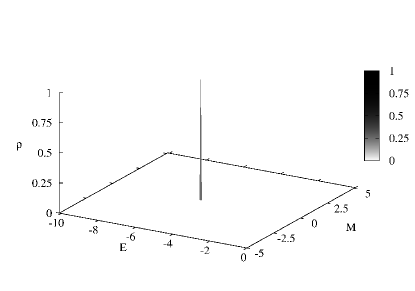
Figure 1: Invariant density $\rho$ on the invariant zero–dipole manifold, projected on a rectangle of the ($E,M$) plane, of energy and angular momentum.

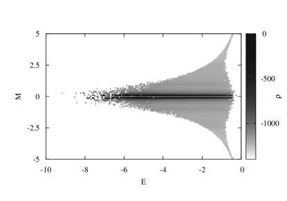
Figure 2: Same as Figure 1, with the values of $\rho$ represented in a gray decimal logarithmic scale, covering a thousand orders of magnitude.

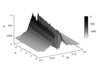
Figure 3: Same as Figure 1, restricted to a smaller portion of the original rectangle, with the ordinates in a decimal logarithmic scale as in Figure 2 .

Now, the zero–dipole manifold is 4–dimensional, so that in principle $\rho$ depends on four variables (i.e., position and velocity). Recall however that on such a manifold the motion is a purely Coulomb one, so that it is integrable. Then, thinking in terms of action–angle variables, the interesting ones are just the two actions, which in our case are $E^{-1/2}$, $\ E$ being the (mechanical) energy, and the angular momentum $M$, whereas the angles, i.e., the orientation of the orbit and the starting point of the motion on the orbit, are irrelevant. So we chose to integrate away the two angles from the density $\rho$, and to analyze the corresponding reduced density, $\rho(E,M)$ (by abuse of language still denoting it by $\rho$).

The result is shown in Figures 1–3. In Figure 1 the reduced density $\rho$ is reported versus $E$ and $M$. While a priori the measure could be spread over the whole rectangle, the figure shows that it is actually concentrated in an extremely small area. This is more clearly exhibited in Figure 2, which still covers the whole rectangle, but gives the density in a decimal lograthmic gray scale, which covers a thousand orders of magnitude. Figure 3 is instead the same as Figure 1, restricted to a smaller portion of the rectangle, still with the ordinates in a decimal logarithmic scale. It shows that the function $\rho(E,M)$ has a very complex structure, with values ranging over a thousand orders of magnitude in an apparently nonsmooth way. This fact might suggest that the measure is not absolutely continuous with respect to the restriction of the Lebesgue one, possibly having some kind of fractal structure, but we leave this problem for possible future work.

In any case, we have shown that the peculiar character of dissipation entering electrodynamics of point particles restricted to the Dirac physical manifold, makes the final dynamics quite different from that of more familiar dissipative systems such as the Lorenz one. Indeed in the latter case it is the invariant attractor that has a strange character, while the natural invariant measure induced on by the dynamics is somehow trivial, as corresponding to that of a hyperbolic system. In the former case, instead, the invariant manifold is trivial (being just the hyperplane ${{\mathbf{x}}}_{cm}=0,\dot{{\mathbf{x}}}_{cm}=0,\ddot{{\mathbf{x}}}_{cm}=0$ in the ambient phase space), while it is the invariant measure which apparently has a strange character.

IV Conclusions

We investigated the main modifications that are introduced in the Coulomb Helium atom model when the radiation reaction forces are taken into account in the simplest possible way, and the asymptotic Dirac prescription is consequently introduced, according to which the phase space has to be restricted to the submanifold of points leading to motions with a finite emitted energy.

The first qualitative result we found is that the problem of the breakdown of the atom (corresponding to autoionization for generic initial data with negative energy), which makes the Coulomb model inconsistent, is now eliminated. The second one is the existence of an invariant manifold of stable periodic orbits, that moreover is attractive. Such a manifold is the zero–dipole one, on which the system does not radiate energy away, in the dipole approximation.

Finally, the invariant measure naturally induced by the time–flow on the zero–dipole manifold was studied numerically. We showed that such a measure is far from trivial, being presumably non absolutely continuous with respect to the restriction of the Lebesgue measure, possibly with some kind of fractal structure. This is at variance with the known examples of dissipative systems, for which the measure is trivial, while it is the attractor that is strange (i.e. a fractal set). This is apparently a consequence of the peculiar character of the radiation reaction force, which makes the system dissipative when restricted to the Dirac physical manifold, while making it expansive in the ambient phase space.

A very interesting problem that remains open is that of comparing the special periodic orbits which are selected on the zero–dipole manifold as the most probable ones according to the natural measure, with those, apparently of special physical relevance, studied by De Luca. We leave this point for future work.

- (1) J. W. Nicholson, Mon. Not. Roy. Ast. Soc. 72, 49 (1911).
- (2) N. Bohr, Phil. Mag. 26, 477 (1913).
- (3) I. Langmuir, Phys. Rev. 17, 339 (1921).
- (4) M. Poirier, Phys. Rev. A 40, 3498 (1989).
- (5) T. Yamamoto, K. Kaneko, Phys. Rev. Lett. 70, 1928 (1993).
- (6) T. Yamamoto, K. Kaneko, Prog. Theor. Phys. 100, 1089 (1998).
- (7) J. De Luca, Phys. Rev. Lett. 80, 680 (1998).
- (8) J. De Luca, Phys. Rev. E 58, 5727 (1998).
- (9) E.N. Lorenz, J. of Atm. Sci. 20, 130 (1963).
- (10) L.D. Landau, E.M. Lifshitz, The Classical Theory of Fields (Pergamon Press, Oxford 1962).
- (11) J.D. Jackson, Classical electrodynamics (Wiley, New York 1975).
- (12) P.A.M. Dirac, Proc. R. Soc. A 167, 148 (1938).
- (13) O.E. Lanford III, Qualitative and statistical theory of dissipative systems, in Statistical mechanics, G. Gallavotti ed., CIME Summer School 71, 24 (Springer, Berlin 2011).
- (14) W. Pauli, Pauli Lectures on Physics - vol 1 (MIT Press, Cambridge 1973).
- (15) W. Heitler, The Quantum Theory of Radiation (Clarendon Press, Oxford 1966).
- (16) J.K. Hale, A.P. Stokes, J. Math. Phys. 3, 70 (1962).
- (17) R. Haag, Z. Naturforsch. A 10, 752 (1955).
- (18) A. Carati, P. Delzanno, L. Galgani, J. Sassarini, Nonlinearity 8, 65 (1995).
- (19) A. Carati, J. Phys. A 34, 5937 (2001).
- (20) M. Marino, J. Phys. A 36, 11247 (2003).
- (21) N.M. Krylov, N.N. Bogolyubov, Annals of Math. 38, 65 (1937).