Non-equilibrium fluctuations in a driven stochastic Lorentz gas

Abstract

We study the stationary state of a one-dimensional kinetic model where a probe particle is driven by an external field $\mathcal{E}$ and collides, elastically or inelastically, with a bath of particles at temperature $T$. We focus on the stationary distribution of the velocity of the particle, and of two estimates of the total entropy production $\Delta s_{tot}$. One is the entropy production of the medium $\Delta s_{m}$, which is equal to the energy exchanged with the scatterers, divided by a parameter $\theta$, coinciding with the particle temperature at $\mathcal{E}=0$. The other is the work $W$ done by the external field, again rescaled by $\theta$. At small $\mathcal{E}$, a good collapse of the two distributions is found: in this case the two quantities also verify the Fluctuation Relation (FR), indicating that both are good approximations of $\Delta s_{tot}$. Differently, for large values of $\mathcal{E}$, the fluctuations of $W$ violate the FR, while $\Delta s_{m}$ still verifies it.

I Introduction

The program of statistical mechanics, consisting in deriving macroscopic properties of a system from the elementary interactions of its constituents, is far from being fulfilled in out-of-equilibrium conditions. In particular, the dissipation of energy in such cases prevents the use of general equilibrium results, and forces one to rely on a case-by-case model-dependent description.

One of the few general results for systems far from equilibrium has been established in a series of works, starting from the seminal papers by Evans and coworkers Evans et al. (1993). It consists in a family of relations, generally referred to as Fluctuation Relations (FR), which are very similar in form, but concern different quantities (e.g. phase space contraction rate, entropy production, heat, work, etc.) and/or different dynamical regimes (e.g. transients, stationary states, etc.), as well as different kinds of non-equilibrium systems, either deterministic or stochastic (see Marconi et al. (2008) and references therein).

In the framework of stochastic dynamics, the microscopic definition of the entropy production relies on the knowledge of the path probabilities for the model Kurchan (1998); Lebowitz and Spohn (1999); Maes (1999); Crooks (1999); Hatano and Sasa (2001); Speck and Seifert (2005); Andrieux and Gaspard (2007). The study of the fluctuations of this quantity plays a central role in the characterization of small systems Bustamante et al. (2005); Collin et al. (2005). The connection with macroscopic quantities that are reasonably related to the thermodynamic concept of “entropy produced by the system” has to be carefully investigated in each specific model, as for instance in Feitosa and Menon (2004); Andrieux et al. (2007); Sarracino et al. (2010a). In particular, the simple recipe, useful near equilibrium, where the macroscopic entropy production is expressed as the work done by external forces divided by the temperature de Groot and Mazur (1984), is hardly of use far from equilibrium, often because it is not clear which parameter plays the role of temperature Cugliandolo (2011). For instance, in granular gases, due to the dissipative character of interactions, the kinetic temperature $T_{g}$ of the microscopic constituents does not always have a thermodynamic role Baldassarri et al. (2005).

In order to address such issues, we investigate the dynamics of a stochastic Lorentz-like model where a particle is interacting with random scatterers and is subjected to an external force. Stochastic Lorentz models have been previously studied, focusing on transport properties, e.g. on normal or anomalous diffusion, for instance in van Beijeren (1982); Bouchet et al. (2004); Mátyás and Gaspard (2005); Giardinà et al. (2006); Karlis et al. (2006); D’Alessio and Krapivsky (2011). Our model is based on the following ingredients: 1) the presence of an external field $\mathcal{E}$ accelerating the probe particle, 2) scatterers of finite mass which are randomly and uniformly distributed in space and move with random velocities as extracted from a thermal bath at temperature $T$ (it is therefore more reasonable to call them “bath particles”), 3) collisions which can also be inelastic (the system always reaches a stationary state), 4) a uniform collision probability which is inspired from the so-called Maxwell-molecules models Ernst (1981), and which helps in simplifying analytical calculations. Such ingredients provide a system in a non-equilibrium stationary state (NESS), due to the presence of a finite stationary current of particles. We do not consider any time-dependent experimental protocol neither any transformation between different NESS, that is, we study the system at fixed value of the external parameter (the external field). For each value of the external field, we start our measurements when the system has already reached the corresponding NESS. Therefore, in our case, there is not excess heat due to transient dynamics between different NESS and the total heat exchanged equals the power dissipated to sustain the NESS.

We show that, in this model, the microscopic entropy production is well approximated, at large times, by the energy exchanged with the bath, divided by a “temperature” $\theta$ which is that measured for zero field, $\mathcal{E}=0$. Such a temperature turns out to be different from the temperature of scatterers $T$, unless the collisions are elastic, and coincides with the one of the probe particle in the unperturbed process, in agreement with what recently found in Evans et al. (2011); at small values of the field, a macroscopically accessible quantity well approximates the entropy production, and that is the work done by the external field, divided by the same temperature $\theta$.

II The model

We consider an ensemble of probe particles of mass $m$ endowed with scalar velocity $v$. Each probe particle only interacts with particles of mass $M$ and velocity $V$ extracted from an equilibrium bath at temperature $T$: such scatterers are distributed randomly and uniformly in space and can hit the particle only once. The last condition is important to guarantee unbounded motion and molecular chaos even in one dimension, and can be thought as the effect of bath particles moving in two (or more) dimensions, while the probe particle can only move along a one-dimensional track. Inspired from Maxwell-molecules models Ernst (1981) and to their inelastic generalization Ben-Naim and Krapivsky (2000); Baldassarri et al. (2002); Ernst and Brito (2002), we assume that the scattering probability does not depend on the relative velocity of colliders. Velocity of the particle changes from $v$ to $v^{\prime}$ at each collision, according to the rule:

$$v^{\prime}=\gamma v+(1-\gamma)V,$$ (1)

where

$$\gamma=\frac{\zeta-\alpha}{1+\zeta}$$ (2)

with $\zeta=m/M$, and $\alpha$ is the coefficient of restitution determining if the collision is elastic $\alpha=1$ or inelastic $\alpha\in[0,1)$. The velocity $V$ of the bath particles is a random variable generated from a Gaussian distribution with zero mean and variance $T/M$:

$$P_{S}(V)=\sqrt{\frac{M}{2\pi T}}\exp\left(-\frac{M}{2T}V^{2}\right).$$ (3)

In addition, the probe particle is accelerated by a uniform force field $m\mathcal{E}$. The resulting system can be assimilated to a Lorentz gas model, where free flights in external field are interrupted by random collisions with scatterers.

The model is summarized by the linear Boltzmann equation for the evolution of the velocity distribution of the probe particle

$$\tau_{c}\partial_{t}P(v,t)+\tau_{c}\mathcal{E}\partial_{v}P(v,t)=$$

$$-P(v,t)+\frac{1}{1-\gamma}\int\!\!\!du\,P(u,t)P_{S}\left(\frac{v-\gamma u}{1-\gamma}\right),$$ (4)

where $\tau_{c}$ is the mean collision time. In the following, we shall compare analytical predictions with numerical simulations of Eq. (II). This equation, restricted to the particular case $\alpha=1$ and $m=M$ (that is $\gamma=0$), has been recently studied in Alastuey and Piasecki (2010).

III Entropy production

One of the most interesting features peculiar to out-of-equilibrium stationary dynamics is that a finite rate of entropy production can be measured in the system. Microscopically, such a quantity is related to the violation of detailed balance and gives a measure of how the probability of observing a forward trajectory differs from the probability of observing the time-reversed one Kurchan (1998); Lebowitz and Spohn (1999). From the macroscopic point of view, the entropy production is related to the presence of currents going through the system, due to spatial gradients or due to the action of external driving forces de Groot and Mazur (1984); Schnakenberg (1976). In simple examples Lebowitz and Spohn (1999); Astumian (2006), a bridge between the two points of view can be verified, where the microscopic entropy production turns out to be proportional to the product of a flux by a force. The constant prefactor, in driven systems in contact with a reservoir, is often found to be the bath temperature. However this cannot be the general situation: for instance, for arbitrarily strong external fields, the temperature of the system (e.g. the kinetic one) may be far from that of the bath, or in extreme cases, cannot even be defined.

The stochastic process considered here consists of two parts: a deterministic evolution, due to the action of the external field, plus a random contribution, due to the collisions with the scatterers. Here, the deterministic process does not contribute to the entropy production in the system, since the probability of a free fall for the particles is symmetric under time-reversal. It is then convenient to rewrite Eq. (II) as a Master Equation where the transition rates describing the stochastic collisions between particles explicitly appear

$$\tau_{c}\partial_{t}P(v,t)+\tau_{c}\mathcal{E}\partial_{v}P(v,t)=$$

$$\int_{-\infty}^{\infty}dv^{\prime}w(v|v^{\prime})P(v^{\prime},t)-\int_{-\infty}^{\infty}dv^{\prime}w(v^{\prime}|v)P(v,t),$$

(5)

with

$$w(v^{\prime}|v)=\frac{1}{1-\gamma}\frac{1}{\sqrt{2\pi T/M}}\exp\left\{-\frac{M}{2T}\left[\frac{v^{\prime}+\gamma v}{1-\gamma}\right]^{2}\right\}.$$ (6)

To obtain this result we have put in Eq. (II) the form (3) for the distribution of the scattering particles (see Ref Puglisi et al. (2006a) for the general case, with different interaction kernels and arbitrary dimension).

For the process described by Eq. (5), we can explicitly write the probability density $P[\{v(t)\}|v_{0}]$ of observing the trajectory $\{v(s)\}_{s=t_{0}}^{t}$ in the interval $[t_{0},t]$, with initial and final values $v(t_{0})=v_{0}$ and $v(t)=v_{t}$, respectively. The total entropy production associated with each trajectory is defined as

$$\Delta s_{tot}(t)=\log\frac{P[\{v(t)\}|v_{0}]P(v_{0})}{P[\{\tilde{v}(t)\}|\tilde{v}_{0}]P(\tilde{v}_{0})}=\Delta s_{m}(t)+\log\frac{P(v_{0})}{P(-v_{t})},$$ (7)

with $\{\tilde{v}(s)=-v(t-s)\}_{s=t_{0}}^{t}$ the time-reversed path, $P(v)$ the stationary distribution and $\Delta s_{m}$ the entropy production of the medium Seifert (2005), where as medium we refer to the ensemble of scatterers. Notice that in the reversed protocol the electric field does not change the sign, $\tilde{\mathcal{E}}=\mathcal{E}$. Along a trajectory where $N_{c}$ collisions occur at times $t_{j}$ (with $j\in[1,N_{c}]$) and velocities change from $v_{j}=v(t_{j}^{-})$ to $v_{j}^{\prime}=v(t_{j}^{+})$ one has

$$\frac{P[\{v(t)\}|v_{0}]}{P[\{\tilde{v}(t)\}|\tilde{v}_{0}]}=\frac{\prod_{j=1}^{N_{c}}P_{nc}(\Delta t_{j})w(v^{\prime}_{j}|v_{j})}{\prod_{j=1}^{N_{c}}P_{nc}(\Delta t_{j})w(-v_{j}|-v^{\prime}_{j})},$$ (8)

where $P_{nc}(\Delta t_{j})$ is the probability that no collision occurs in the time interval $\Delta t_{j}=t_{j}-t_{j-1}$. Since in the Maxwell model the collision probability is independent of the particle velocity, the time intervals $\Delta t_{j}$ between successive collisions are distributed according to a Poissonian process with $P_{nc}(\Delta t_{j})\sim\exp(-\Delta t_{j}/\tau_{c})$. In the ratio between probabilities appearing in Eq. (8), the contributions due to free flights in the backward trajectory exactly cancel those coming from the forward trajectory. It is interesting to mention that such cancellation is not a specific feature of the chosen uniform collision probability: it can be verified also for other kinds of interactions, e.g. for hard spheres.

The stochastic entropy production of the medium is then expressed in terms of single event contributions $\delta s_{m}(v^{\prime},v)$, where the particle changes its velocity from $v$, before the collision, to $v^{\prime}$, after the collision,

$$\Delta s_{m}(t)=\sum_{j=1}^{N_{c}(t)}\delta s_{m}(v^{\prime}_{j},v_{j}).$$ (9)

Here $N_{c}(t)$ is the number of collisions occurred up to time $t$ and, from Eq. (6),

$$\delta s_{m}(v^{\prime}_{j},v_{j}) = \log\frac{w(v^{\prime}_{j}|v_{j})}{w(-v_{j}|-v^{\prime}_{j})}$$ (10)

$$= -\frac{M(1+\gamma)}{2T(1-\gamma)}(v^{\prime 2}_{j}-v_{j}^{2})$$

$$= -\frac{\delta E_{coll}(v^{\prime}_{j},v_{j})}{\theta},$$

where $\delta E_{coll}(v^{\prime}_{j},v_{j})=m/2(v^{\prime 2}_{j}-v_{j}^{2})$ is the energy received from the scatterers in a collision and

$$\theta=T\zeta\frac{1-\gamma}{1+\gamma}=T\zeta\frac{1+\alpha}{1+2\zeta-\alpha}$$ (11)

is the kinetic temperature of the probe particle in zero field, as demonstrated below (see Eq. (24)).

For the average rate of entropy production in a stationary state we can write

$$\langle\dot{s}_{m}(t)\rangle = \lim_{t\rightarrow\infty}\frac{\langle\Delta s_{m}(t)\rangle}{t}=\frac{1}{\tau_{c}}\left\langle\delta s_{m}(v^{\prime},v)\right\rangle$$

$$= -\frac{1}{\tau_{c}}\frac{M(1+\gamma)}{2T(1-\gamma)}(\langle v^{\prime 2}\rangle_{post}-\langle v^{2}\rangle),$$

where $\langle\cdots\rangle_{post}$ denotes the average over the distribution of post-collision velocities. In order to compute explicitly the average quantities appearing in Eq. (LABEL:entropy), we need to solve the Boltzmann equation (II) in the stationary limit.

IV Stationary solution

Defining the Fourier transform of the probability density $\hat{P}(k,t)=\int_{-\infty}^{\infty}dve^{ikv}P(v,t)$ and similarly for $\hat{P}_{S}(k)$, the integral equation (II) in Fourier space in the stationary limit assumes the convenient form:

$$-ik\mathcal{E}\tau_{c}\hat{P}(k)=-\hat{P}(k)+\hat{P}(\gamma k)\hat{P}_{S}((1-\gamma)k).$$ (13)

Let us start by considering the simplest case $\gamma=0$. This corresponds to $\zeta=\alpha$ and it has been considered in Alastuey and Piasecki (2010); Gervois and Piasecki (1986), for elastic particles with $m=M$. Since $\hat{P}(0)=1$, from Eq. (13) we have

$$\hat{P}(k)=\frac{1}{1-i\mathcal{E}\tau_{c}k}\hat{P}_{S}(k)=\frac{1}{1-i\mathcal{E}\tau_{c}k}\exp\left(-\frac{T}{2M}k^{2}\right).$$ (14)

The inversion of the Fourier transform gives the sought distribution under the form of a convolution:

$$P(v)=b\sqrt{\frac{a}{\pi}}\int_{0}^{\infty}du\exp(-a(v-u)^{2})\times\exp(-bu),$$ (15)

with $b=\frac{1}{\tau_{c}\mathcal{E}}$ and $a=\frac{M}{2T}$. The result of the convolution is that the tails for large $v$ are exponential and for negative $v$ are Gaussian. In the limit of infinite mass of the scatterers, $M\to\infty$, the distribution becomes one sided and reads:

$$P(v)=\theta(v)\frac{1}{\tau_{c}\mathcal{E}}\exp\left(-\frac{v}{\tau_{c}\mathcal{E}}\right).$$ (16)

In Fig. 1 the analytical prediction of Eq. (15) is compared with the pdf obtained in numerical simulations (see below).

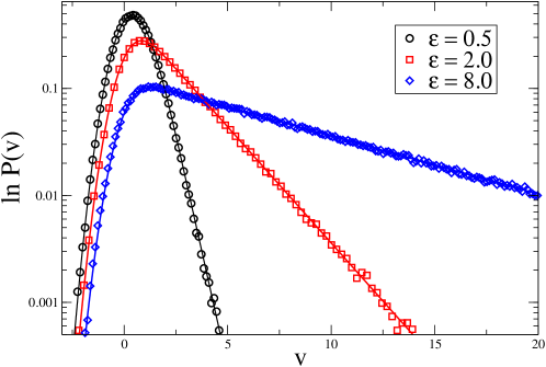
Figure 1: (Color online) Comparison between the theoretical prediction of Eq. (15) (solid lines) and the numerical simulations (symbols) for the stationary distribution in the case $\gamma=0$, $\tau_{c}=1$, $\zeta=0.5$, $T=1$ and for different values of the external field $\mathcal{E}=0.5,2,8$.

For arbitrary values of $\gamma$, equation (13) can be easily solved in the case of zero field $\mathcal{E}=0$, where one has

$$\hat{P}_{0}(k)=\exp\left(-\frac{\theta}{2m}k^{2}\right),$$ (17)

with a temperature $\theta$. Notice that $P_{0}(v)$ is a Maxwellian, but with a “temperature” $\theta$ which differs from $T$; one has $\theta=T$ only when $\alpha=1$. In the presence of non-zero field, no analogue of the closed formula (15) can be written. However, in this case one has access to all the moments of the distribution. Indeed, assuming analyticity around $k=0$, for small enough $k$ one can write the expansion

$$\hat{P}(k)=\sum_{n=0}^{\infty}\frac{(ik)^{n}}{n!}\mu_{n},$$ (18)

where $\mu_{n}\equiv\langle v^{n}\rangle$. Upon substituting expression (18) in Eq. (13), and equating equal powers of $k$, all the moments of the distribution can be obtained. In particular, using Eq. (3), we have

$$\mu_{1}=\frac{\tau_{c}\mathcal{E}}{1-\gamma}$$ (19)

$$\mu_{2}=\frac{2\tau_{c}\mathcal{E}}{1-\gamma^{2}}\mu_{1}+\frac{(1-\gamma)^{2}}{1-\gamma^{2}}\mu^{(S)}_{2}.$$ (20)

It is interesting to note that the conductibility $\langle v\rangle/\mathcal{E}=\tau_{c}/(1-\gamma)\equiv\tau_{c}(1+\zeta)/(1+\alpha)$ increases when the system becomes more inelastic ($\alpha$ reduced) or when the mass $M$ of the bath particles is reduced.

We are now ready to compute the average entropy production. Indeed, substituting Eq. (20) in Eq. (LABEL:entropy), and using the fact that the distribution of post-collisional velocities is by definition $\hat{P}_{post}(k)=\hat{P}(\gamma k)\hat{P}_{S}((1-\gamma)k)$, we can write

$$\langle\dot{s}_{m}(t)\rangle=\frac{(1+\gamma)}{(1-\gamma)^{2}}\frac{M}{T}\tau_{c}\mathcal{E}^{2}\geq 0.$$ (21)

Expression (21) can be related to the macroscopic quantities present in the system, namely the external field $\mathcal{E}$ and the current velocity $\langle v\rangle$. Indeed, using Eq. (11), Eq. (21) can be rewritten as

$$\langle\dot{s}_{m}(t)\rangle=\frac{m}{\theta}\frac{\tau_{c}\mathcal{E}^{2}}{(1-\gamma)}=\frac{m\mathcal{E}\langle v\rangle}{\theta}\geq 0.$$ (22)

Now let us consider the average work done by the external field along a trajectory that spans the time interval $[0,t]$, $W(t)=\int_{0}^{t}Fv(s)ds$, with $F=m\mathcal{E}$:

$$\lim_{t\to\infty}\frac{1}{\theta}\frac{\langle W(t)\rangle}{t}=\frac{F\langle v\rangle}{\theta}=\langle\dot{s}_{m}(t)\rangle,$$ (23)

i.e. the average macroscopic work of the field divided by the temperature $\theta$ corresponds to the average entropy production. Notice that in Eq. (23) the “right” temperature is neither the bath temperature $T$, nor the kinetic temperature of the probe particle in the presence of the field

$$T_{g}\equiv m\Bigl{(}\mu_{2}-\mu_{1}^{2}\Bigr{)}=\theta+m\frac{(\tau_{c}\mathcal{E})^{2}}{(1-\gamma^{2})},$$ (24)

but it is that of the unperturbed, not accelerated system. The quantity $\theta$ represents an energy scale in the system, which depends on the several parameters defining the model, namely temperature of the scatterers $T$, mass ratio $\zeta$ and restitution coefficient $\alpha$. It is equal to the kinetic temperature of the particle only in the absence of external field. In this case, if the interactions are elastic, it equals the bath temperature $T$, as expected. In general, for non zero field, the relation between $\theta$ and the mean square velocity of the particle is expressed by Eq. (24).

V Numerical simulations

In order to obtain numerically the stationary distribution $P(v)$ which solves Eq. (II), we simulate the dynamics of a single particle subject to a constant acceleration $\mathcal{E}$ and to inelastic collisions with the scatterers, and average over $10^{4}$ realizations, for general $\gamma$. Time is discretized in intervals $\delta t$, for a total duration $\delta tN_{t}$. The particle is accelerated for $\delta t$ under the influence of the constant field $\mathcal{E}$ and then a collision with a scatterer is realized with probability $p_{coll}=\delta t/\tau_{c}$. The distinguishing feature of Maxwell molecules Ernst (1981) is that the probability of colliding is independent of the velocity of the particle itself. Then, the particle is again uniformly accelerated by the field $\mathcal{E}$ and the whole procedure is repeated. This ensures an average collision time $\tau_{c}$, which is set as a parameter of the simulation. For each collision the velocity of the scatterers are extracted from a constant Gaussian distribution, Eq. (3), and the collision with the probe particle is realized with the inelastic rule, Eq. (1).

In the numerical simulations we also studied the diffusive properties of the system to find that the mean square displacement with respect to the average motion, $d_{2}=\langle[x(t)-\langle x(t)\rangle]^{2}\rangle$, displays a ballistic behavior $d_{2}\sim t^{2}$ on short time scales with a crossover to a diffusional dynamics $d_{2}\sim t$ at large times. Such a ballistic-to-diffusive scenario, not intuitive in the presence of an accelerating field Bouchet et al. (2004); Karlis et al. (2006), is consistent with the autocorrelation of the particle’s velocity which, up to numerical precision, decays as a single exponential.

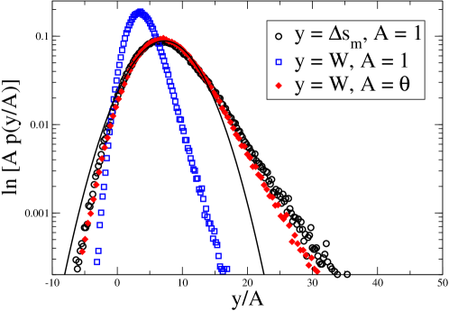
Figure 2: (Color online) PDF of entropy production, work and rescaled work. Parameters: $\gamma=0$, $\tau_{c}=1$, $\zeta=0.5$, $T=1$, $\mathcal{E}=0.5$ and $t=16\tau_{c}$. The continuous line shows the Gaussian fit of $p(\Delta s_{m})$.

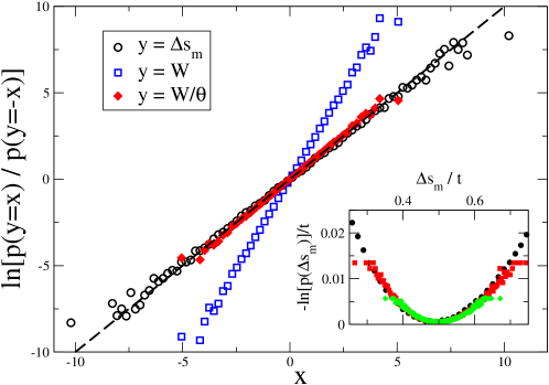
Figure 3: (Color online) The symmetry relation (26) obeyed by the entropy production $\Delta s_{m}(t)$ and by the rescaled work $W(t)/\theta$ obtained in numerical simulations with parameters: $\gamma=0$, $\tau_{c}=1$, $\zeta=0.5$, $T=1$, $\mathcal{E}=0.5$ and $t=16\tau_{c}$. Inset: collapse of the rate functions of the distribution of $\Delta s_{m}(t)$ for large times $t=128\tau_{c}$ (black circles), $t=512\tau_{c}$ (red squares) and $t=1024\tau_{c}$ (green diamond).

VI The role of inelasticity

A peculiarity of this model is that the inelastic collision rule can be always mapped onto an elastic one: indeed we can always set $\alpha=1$ and change the mass ratio $\zeta=m/M$ in order to keep constant the parameter $\gamma$ which enters the collision rule. In practice, if also $m$ is kept fixed, we are changing only $M$ and thus the width of the distribution in Eq. (3). Doing so we find no relevant qualitative change in the physics of the system. In particular, let us notice that the entropy production in Eq. (21) depends only on $\gamma$ and vanishes with the field $\mathcal{E}$, also with inelastic collisions.

The fact that, for the present model, the entropy production is not affected by the inelasticity of collisions is in agreement with the findings of Sarracino et al. (2010b), where the dynamics of a single massive intruder in a diluted granular gas of inelastic particles satisfying the molecular chaos hypothesis was studied. In that case the dynamics of the probe particle was well described by a single linear Langevin equation, so that the entropy production was zero by definition. Without passing through a Langevin description, also the Maxwell model presented here assumes the molecular chaos hypothesis for the surrounding sea of scatterers. In both cases each collision of the probe particle is performed with a velocity extracted from a constant distribution independent of the previous history of the system: despite the inelasticity of collisions, reversibility is guaranteed by the molecular chaos hypothesis for the medium. As it is clear from Eq. (21), in our model all irreversible effects are generated by the external field.

There is only one special case in which the entropy production allows us to distinguish the inelastic from the elastic interaction. This is the case of infinitely massive scatterers, namely $M\rightarrow\infty$, which implies $\zeta=0$ and $\gamma=-\alpha$. Keeping finite the width of the velocity distribution of scatterers, $T/M=\mu_{2}^{(S)}$, the average entropy production then reads

$$\langle\dot{s}_{m}(t)\rangle=\frac{1-\alpha}{1+\alpha}\frac{\tau_{c}\mathcal{E}^{2}}{\mu_{2}^{(S)}},$$ (25)

namely it vanishes in the elastic case. This case is quite peculiar because its stationary $P(v)$ has finite $\langle v\rangle$ but infinite $\langle v^{2}\rangle$ Alastuey and Piasecki (2010). For any other parameters the model has finite or zero current and finite energy.

VII Fluctuations of entropy production and work

By definition the total entropy production (7) must satisfy the FR for any value of $t$:

$$\log\frac{p(\Delta s_{tot}(t)=x)}{p(\Delta s_{tot}(t)=-x)}=x,$$ (26)

with $p(\Delta s_{tot}(t)=x)$ the probability density that in a time interval $[0,t]$ the entropy produced by the system is $x$. At large times $t$, one usually neglects the term $\log[P(v_{0})/P(-v_{t})]$ which - in the definition of $\Delta s_{tot}(t)$ - gives a contribution of order $\mathcal{O}(1)$, and looks for the fulfillment of Eq. (26) using $\Delta s_{tot}(t)\approx\Delta s_{m}(t)$, which should be the leading part of order $\mathcal{O}(t)$. Our numerical simulations suggest that this is the case also in this model, for any value of the field $\mathcal{E}$. As seen in Eqs. (9)-(10), $\Delta s_{m}(t)$ coincides with the energy that the probe particle loses when colliding with the bath particles, divided by the kinetic temperature of the particle itself measured at zero field. In Fig. 2 the distribution of $\Delta s_{m}(t)$ is plotted for a certain value of $t$: it can be clearly seen from the superimposed fit a remarkable deviation from gaussianity.

Inspired from the equality of the average value of the entropy and of the work produced along a trajectory, see Eq. (23), we measured in numerical simulation also the fluctuations of the work done by the external field on the particle, $W(t)$. A remarkable finding is that, for small values of $\mathcal{E}$, the PDF of the work can be collapsed on the PDF of the entropy production by exploiting the “unperturbed” temperature $\theta$ as a scaling parameter. In such cases, the measure of work fluctuations provides an alternative way to measure the temperature of the unperturbed system: indeed, as also verified in Fig. 3, when $W(t)/\theta$ satisfies the FR, one also has $\log[p(W(t)=x)/p(W(t)=-x)]=x/\theta$.

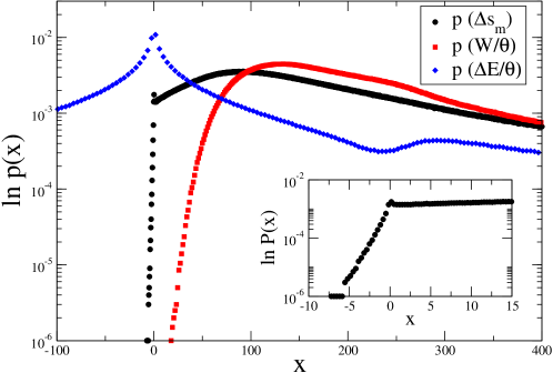
Figure 4: (Color online) PDF of the quantities $\Delta s_{m}$, $W/\theta$ and $\Delta E/\theta$ measured in numerical simulations with parameters: $\gamma=0$, $\tau_{c}=1$, $\zeta=0.5$, $T=1$, $\mathcal{E}=8$ and $t=16\tau_{c}$. Inset: zoom of the region around $x=0$ for the probability distribution of $\Delta s_{m}$.

By increasing the value of $\mathcal{E}$ while keeping fixed all the other parameters of the simulation we find the following differences with the small $\mathcal{E}$ situation: a) the stationary PDF of velocity has a larger exponential tail and a very asymmetric shape; b) the PDF of $\Delta s_{m}(t)$ also becomes very asymmetric and close to 0 has a shape very different from a Gaussian one, see inset of Fig. 4; c) the PDF of $W(t)$ cannot be collapsed on the PDF of the entropy production with a simple rescaling; d) $\Delta s_{m}(t)$ still verifies the FR, while $W(t)/\theta$ does not.

The breaking of the FR symmetry by the fluctuations of work at large values of $\mathcal{E}$ can be interpreted considering the balance equations of the energy absorbed and lost by the probe particle within a time window. In particular, we have that $W(t)+\Delta E_{coll}(t)=\Delta E(t)$, with $\Delta E(t)=\frac{m}{2}[v^{2}(t)-v^{2}(0)]$ and $\Delta E_{coll}(t)=\sum_{j=1}^{N_{c}(t)}\delta E_{coll}(v^{\prime}_{j},v_{j})$ and therefore, exploiting the relation (10), we can write:

$$\Delta s_{m}(t)=\frac{1}{\theta}\left[W(t)-\Delta E(t)\right],$$ (27)

which puts in evidence that discrepancies between the distribution of $\Delta s_{m}$ and $W/\theta$ are due to the “boundary term” $\Delta E$. Although $\Delta E(t)$ is of order $\mathcal{O}(1)$, it is known to be dangerous for FR, even at large times, when its distribution has exponential (or larger) tails van Zon and Cohen (2003); Puglisi et al. (2006b), as in our case (see Fig. 4).

In summary, we have discussed a non-equilibrium kinetic model, simple enough to let most of the calculations accessible, such as the entropy production or the moments of the stationary distribution, but still displaying interesting properties, for instance strong non-Gaussian behavior and non-trivial dependence on the external field. In particular we have seen that the Fluctuation Relation is valid for the distribution of the energy $\Delta E_{coll}$ lost in collisions with the bath, and it also holds for the work done by the field, $W(t)$, provided that $\mathcal{E}$ is low enough. For the fulfillment of the FR, both quantities have to be divided by a temperature $\theta$ which is different from the bath and the particle ones, but coincides with the latter at $\mathcal{E}=0$. We remark that such an observation is highly non-trivial: it suggests that extreme care must be used when entropy production is defined on phenomenological grounds, where one is usually tempted to use more “reasonable” temperatures (e.g. the bath or the system ones), forgetting the complexity of far-from-equilibrium systems.