Resolving conflicts between statistical methods by probability combination: Application to empirical Bayes analyses of genomic data

Abstract

In the typical analysis of a data set, a single method is selected for statistical reporting even when equally applicable methods yield very different results. Examples of equally applicable methods can correspond to those of different ancillary statistics in frequentist inference and of different prior distributions in Bayesian inference. More broadly, choices are made between parametric and nonparametric methods and between frequentist and Bayesian methods. Rather than choosing a single method, it can be safer, in a game-theoretic sense, to combine those that are equally appropriate in light of the available information. Since methods of combining subjectively assessed probability distributions are not objective enough for that purpose, this paper introduces a method of distribution combination that does not require any assignment of distribution weights. It does so by formalizing a hedging strategy in terms of a game between three players: nature, a statistician combining distributions, and a statistician refusing to combine distributions. The optimal move of the first statistician reduces to the solution of a simpler problem of selecting an estimating distribution that minimizes the Kullback-Leibler loss maximized over the plausible distributions to be combined. The resulting combined distribution is a linear combination of the most extreme of the distributions to be combined that are scientifically plausible. The optimal weights are close enough to each other that no extreme distribution dominates the others. The new methodology is illustrated by combining conflicting empirical Bayes methodologies in the context of gene expression data analysis.

David R. Bickel

Ottawa Institute of Systems Biology
Department of Biochemistry, Microbiology, and Immunology
Department of Mathematics and Statistics
University of Ottawa; 451 Smyth Road; Ottawa, Ontario, K1H 8M5

Keywords: ancillarity; conditional inference; combining probabilities; combining probability distributions; combining tests in parallel; confidence distribution; confidence posterior; cross entropy; game theory; imprecise probability; inferential gain; Kullback-Leibler information; Kullback-Leibler divergence; large-scale simultaneous inference; linear opinion pool; minimax redundancy; multiple hypothesis testing; multiple comparison procedure; observed confidence level; redundancy-capacity theorem

1 Introduction

The analysis of biological data often requires choices between methods that seem equally applicable and yet that can yield very different results. This occurs not only with the notorious problems in frequentist statistics of conditioning on one of multiple ancillary statistics and in Bayesian statistics of selecting one of many appropriate priors, but also in choices between frequentist and Bayesian methods, in whether to use a potentially powerful parametric test to analyze a small sample of unknown distribution, in whether and how to adjust for multiple testing, and in whether to use a frequentist model averaging procedure. Today, statisticians simultaneously testing thousands of hypotheses must often decide whether to apply a multiple comparisons procedure using the assumption that the p-value is uniform under the null hypothesis (theoretical null distribution) or a null distribution estimated from the data (empirical null distribution). While the empirical null reduces estimation bias in many situations (Efron, 2007), it also increases variance (Efron, 2010) and substantially increases bias when the data distributions have heavy tails (Bickel, 2011d). Without any strong indication of which method can be expected to perform better for a particular data set, combining their estimated false discovery rates or adjusted p-values may be the safest approach.

Emphasizing the reference class problem, Barndorff-Nielsen (1995) pointed out the need for ways to assess the evidence in the diversity of statistical inferences that can be drawn from the same data. Previous applications of p-value combination have included combining inferences from different ancillary statistics (Good, 1984), combining inferences from more robust procedures with those from procedures with stronger assumptions, and combining inferences from different alternative distributions (Good, 1958). However, those combination procedures are only justified by a heuristic Bayesian argument and have not been widely adopted. To offer a viable alternative, the problem of combining conflicting methods is framed herein in terms of probability combination.

Most existing methods of automatically combining probability distributions have been designed for the integration of expert opinions. For example, Toda (1956), Abbas (2009), and Kracík (2011) proposed combining distributions to minimize a weighted sum of Kullback-Leibler divergences from the distributions being combined, with the weights determined subjectively, e.g., by the elicitation of the opinions of the experts who provided the distributions or by the extent to which each expert is considered credible. Under broad conditions, that approach leads to the linear combination of the distributions that is defined by those weights (Toda, 1956; Kracík, 2011).

“Linear opinion pools” also result from this marginalization property: any linearly combined marginal distribution is the same whether marginalization or combination is carried out first (McConway, 1981). The marginalization property forbids certain counterintuitive combinations of distributions, including any combination of distributions that differs in a probability assignment from the unanimous assignment of all distributions combined (Cooke, 1991, p. 173). Combinations violating the marginalization property can be expected to perform poorly as estimators regardless of their appeal as distributions of belief. On the other hand, invariance to reversing the order of Bayesian updating and distribution combination instead requires a “logarithmic opinion pool,” which uses a geometric mean in place the arithmetic mean of the linear opinion pool; see, e.g., Berger (1985, §4.11.1) or Clemen and Winkler (1999). While that property is preferable to the marginalization property from the point of view of a Bayesian agent making decisions on the basis of independent reports of other Bayesian agents, it is less suitable for combining distributions that are highly dependent or that are distribution estimates rather than actual distributions of belief. Genest and Zidek (1986) and Cooke (1991, Ch. 11) review these and related issues.

Like those methods, the strategy introduced in this paper is intended for combining distributions based on the same data or information as opposed to combining distributions based on independent data sets. However, to relax the requirement that the distributions be provided by experts, the weights are optimized rather than specified. While the new strategy leads to a linear combination of distributions, the combination hedges by including only the most extreme distributions rather than all of the distributions. In addition, the game leading to the hedging takes into account any known constraints on the true distribution. See Remark 1 on the pivotal role game theory played in the foundations of statistics.

The game that generates the hedging strategy is played between three players: the mechanism that generates the true distribution (“Nature”), a statistician who never combines distributions (“Chooser”), and a statistician open to combining distributions (“Combiner”). Nature must select a distribution that complies with constraints known to the statisticians, who want to choose distributions as close as possible to the distribution chosen by Nature. Other things being equal, each statistician would also like to select a distribution that is as much better than that of the other statistician as possible. Thus, each statistician seeks primarily to come close to the truth and secondarily to improve upon the distribution selected by the other statistician. Combiner has the advantage over Chooser that the former may select any distribution, whereas the latter must select one from a given set of the distributions that estimate the true distribution or that encode expert opinion. On the other hand, Combiner is disadvantaged in that Nature seeks to maximize the gain of Chooser without concern for the gain of Combiner. Since Nature favors Chooser without opposing Combiner, the optimal strategy of Combiner is one of hedging but is less cautious than the minimax strategies that are often optimal for typical two-player zero-sum games against Nature. The distribution chosen according to the strategy of Combiner will be considered the combination of the distributions available to Chooser. The combination distribution is a function not only of the combining distributions but also of the constraints on the true distribution.

Sec. 2 encodes the game and strategy described above in terms of Kullback-Leibler loss and presents its optimal solution as a general method of combining distributions. The important special case of combining probabilities is then worked out. A framework for using the proposed combination method to resolve method conflicts in point and interval estimation, hypothesis testing, and other aspects of statistical data analysis will be presented in Sec. 3. The framework is illustrated by applying it to the combination of three false discovery rate methods for the analysis of microarray data in Sec. 4. Finally, Appendices A and B collect miscellaneous remarks and proofs, respectively.

2 Framework for combining distributions

2.1 Information-theoretic background

Let $\mathcal{P}$ denote the set of probability distributions on a Borel space $\left(\Xi,\mathcal{B}\left(\Xi\right)\right)$, where $\mathcal{B}\left(\Xi\right)$ is the set of all Borel subsets of $\Xi$. The information divergence of $P\in\mathcal{P}$ with respect to $Q\in\mathcal{P}$ is defined as

$$D\left(P||Q\right)=\int dP\left(\xi\right)\log\frac{dP\left(\xi\right)}{dQ\left(\xi\right)},$$ (1)

where $dP$ and $dQ$ are probability density functions of $P$ and $Q$ in the sense of Radon-Nikodym differentiation with respect to the same dominating measure (Haussler, 1997). The integrand follows the $0\log\left(0\right)=0$ and $0\log\left(0/0\right)=0$ conventions. $D\left(P||Q\right)$ is also known as “information for discrimination,” “Kullback-Leibler information,” “Kullback-Leibler divergence,” and “cross entropy.” Calling $D\left(P||Q\right)$ “information divergence” emphasizes its interpretation as the amount of information that would be gained by replacing any distribution $Q$ with the true distribution $P$. That interpretation accords with calling

$$D\left(P^{\prime}||P^{\prime\prime}\rightsquigarrow Q\right)=D\left(P^{\prime}||P^{\prime\prime}\right)-D\left(P^{\prime}||Q\right)$$ (2)

the information gain (Pfaffelhuber, 1977), the amount of information gained by using $Q$ rather than $P^{\prime\prime}\in\mathcal{P}$ when the true distribution is $P^{\prime}\in\mathcal{P}$ (cf. Topsøe, 2007).

For any real parameter set $\Phi$ and family $\mathcal{P}^{\star}=\left\{P_{\phi}:\phi\in\Phi\right\}$ of probability distributions such that $\mathcal{P}^{\star}\subseteq\mathcal{P}$, the distribution

$$\widetilde{\mathcal{P}^{\star}}=\arg\inf_{Q\in\mathcal{P}}\sup_{P^{\star}\in\mathcal{\mathcal{P}^{\star}}}D\left(P^{\star}||Q\right)$$ (3)

is called the centroid of $\mathcal{P}^{\star}$ (Csiszár and Körner, 2011, p. 131). Let $\mathcal{W}$ denote the set of all measures on the Borel space $\left(\Phi,\mathcal{B}\left(\Phi\right)\right)$. Reserving the term prior for Sec. 3, members of $\mathcal{W}$ will be called weighting distributions. Then $P^{W}=E_{W}\mathcal{P}^{\star}=\int P_{\phi}dW\left(\phi\right)$ defines the mixture distribution of $\mathcal{P}^{\star}$ with respect to some $W\in\mathcal{W}$, and

$$W_{\mathcal{P}^{\star}}=\arg\sup_{W\in\mathcal{W}}\int D\left(P_{\phi}||E_{W}\mathcal{P}^{\star}\right)dW\left(\phi\right)$$ (4)

defines the weighting distribution induced by $\mathcal{P}^{\star}$.

Example 1.

In the case of a family of $\nu$ distributions, the parameter set can be written as $\Phi=\left\{\phi_{1},\dots,\phi_{\nu}\right\}$ and the weighting distribution as

$$\left\langle W_{\mathcal{P}^{\star}}\left(\phi_{1}\right),\dots,W_{\mathcal{P}^{\star}}\left(\phi_{\nu}\right)\right\rangle=\arg\sup_{w_{1}\in\left[0,1\right],\dots,w_{\nu}\in\left[0,1\right]}\sum_{i=1,\dots,\nu}w_{i}D\left(P_{\phi}||\sum_{j=1,\dots,\nu}w_{j}P_{\phi_{j}}\right),$$

where the supremum is that of the set of weight $\nu$-tuples constrained by $\sum_{i=1}^{\nu}w_{i}=1$. Shulman and Feder (2004) proved that, for all $i=1,\dots,\nu$,

$$W_{\mathcal{P}^{\star}}\left(\phi_{i}\right)\leq 1-e^{-1}\doteq 63\%.$$ (5)

$\operatorname{\blacktriangle}$

The next known result will prove useful in determining the optimal move in the game of combining distributions that was mentioned in Sec. 1.

Lemma 1.

The centroid of any nonempty $\mathcal{P}^{\star}\subseteq\mathcal{P}$ is $\widetilde{\mathcal{P}^{\star}}=P^{W_{\mathcal{P}^{\star}}}$, where $W_{\mathcal{P}^{\star}}$ is the weighting distribution induced by $\mathcal{P}^{\star}$.

Proof.

Two different proofs appear in Haussler (1997) and in Grünwald and Philip Dawid (2004). For some history of this result, see Remark 2. ∎

2.2 Distribution-combination game

The game sketched in Sec. 1 will now be specified in the above notation. Two sets constrain moves in the game: the plausible set $\dot{\mathcal{P}}$ is the subset of $\mathcal{P}$ consisting of given plausible distributions, and $\ddot{\mathcal{P}}\subseteq\mathcal{P}$ consists of given combining distributions. The move of Nature is a distribution $\dot{P}\in\dot{\mathcal{P}}$; the move of Chooser is a distribution $\ddot{P}\in\ddot{\mathcal{P}}$; the move of Combiner is a distribution $P^{+}\in\mathcal{P}$. Chooser and Combiner are called statisticians. If $P_{1}$ is the move of one statistician and $P_{2}$ is that of the other, then the amount of utility paid to the latter is the pair

$$U\left(\dot{P},P_{1},P_{2}\right)=\left\langle-D\left(\dot{P}||P_{2}\right),D\left(\dot{P}||P_{1}\rightsquigarrow P_{2}\right)\right\rangle,$$ (6)

understood in terms of preferring $v=\left\langle v_{1},v_{2}\right\rangle\in\left[0,\infty\right)\times\left[0,\infty\right)$ over $u=\left\langle u_{1},u_{2}\right\rangle\in\left[0,\infty\right)\times\left[0,\infty\right)$ if and only if $u\preceq v$. Here, $u\preceq v$ means that either $u_{1}<v_{1}$ or both $u_{1}=v_{1}$ and $u_{2}\leq v_{2}$. Such preferences are said to have lexicographic ordering (Remark 3).

Thus, the utility paid to Combiner will be $U\left(\dot{P},\ddot{P},P^{+}\right)$ and that paid to Chooser will be $U\left(\dot{P},P^{+},\ddot{P}\right)$. The utility paid to Nature will also be $U\left(\dot{P},P^{+},\ddot{P}\right)$, with the implication that it is to the advantage of Nature and Chooser to act as a coalition with move $\left\langle\dot{P},\ddot{P}\right\rangle$ (von Neumann and Morgenstern, 1953, Ch. 5). Although that reduces the three-player game to a two-player game of the coalition versus Combiner, it is not necessarily of zero sum.

The combination of the distributions in $\ddot{\mathcal{P}}$ with truth constrained by $\dot{\mathcal{P}}$ is defined as Combiner’s optimal move in the game. Since the utility paid to the Nature-Chooser coalition is $U\left(\dot{P},P^{+},\ddot{P}\right)$, Combiner’s best move may be written as

$$P^{+}=\arg\sup_{Q\in\mathcal{P}:\left\langle\dot{P}_{Q},\ddot{P}_{Q}\right\rangle\in\mathcal{P}_{Q}}^{\preceq}U\left(\dot{P}_{Q},\ddot{P}_{Q},Q\right)$$ (7)

for all $Q\in\mathcal{P}$, where $\sup^{\preceq}$ is the least upper bound according to $\preceq$, and

$$\mathcal{P}_{Q}=\arg\sup_{\left\langle P^{\prime},P^{\prime\prime}\right\rangle\in\dot{\mathcal{P}}\times\ddot{\mathcal{P}}}^{\preceq}U\left(P^{\prime},Q,P^{\prime\prime}\right).$$ (8)

While $P^{+}$ is not necessarily a plausible distribution, it is typically at the center of the plausible set:

Theorem 1.

Let $P^{+}$ denote the combination of the distributions in $\ddot{\mathcal{P}}$ with truth constrained by $\dot{\mathcal{P}}$. If $\dot{\mathcal{P}}\cap\ddot{\mathcal{P}}\neq\emptyset$, then

$$P^{+}=\widetilde{\dot{\mathcal{P}}\cap\ddot{\mathcal{P}}}=P^{W_{\dot{\mathcal{P}}\cap\ddot{\mathcal{P}}}},$$ (9)

where $\widetilde{\dot{\mathcal{P}}\cap\ddot{\mathcal{P}}}$ is the centroid of $\dot{\mathcal{P}}\cap\ddot{\mathcal{P}}$, and $W_{\dot{\mathcal{P}}\cap\ddot{\mathcal{P}}}$ is the weighting distribution induced by $\dot{\mathcal{P}}\cap\ddot{\mathcal{P}}$, as defined by eq. (4).

Let $\mathcal{A}$ denote an action space. A decision made by taking the action $a\in\mathcal{A}$ that minimizes the expectation value of a loss function $L:\Xi\times\mathcal{A}\rightarrow\mathbb{R}$ with respect to $P^{+}$ is optimal in the game when the utility function of eq. (6) is replaced with

$$\left\langle-D\left(\dot{P}||P_{2}\right),D\left(\dot{P}||P_{1}\rightsquigarrow P_{2}\right),-\int L\left(\xi,a\right)dP_{2}\left(\xi\right)\right\rangle.$$

The latter utility function is understood in terms of the lexicographic ordering relation $\preccurlyeq$, which is defined such that $\left\langle u_{1},u_{2},u_{3}\right\rangle\preccurlyeq\left\langle v_{1},v_{2},v_{3}\right\rangle$ if and only if one of the following is true: (i) $u_{1}<v_{1}$; (ii) $u_{1}=v_{1}$ and $u_{2}<v_{2}$; (iii) $u_{1}=v_{1}$, $u_{2}=v_{2}$, and $u_{3}\leq v_{3}$. On related orderings in the literature, see Remark 3.

2.3 Combining discrete distributions

Now let $\mathcal{P}$ denote the set of probability distributions on $\left(\Xi,2^{\Xi}\right),$ where $\Xi$ is a finite set written as $\Xi=\left\{0,1,...,\left|\Xi\right|-1\right\}$ without loss of generality. Then the information divergence of $P$ with respect to $Q$ (1) reduces to

$$D\left(P||Q\right)=\sum_{i\in\Xi}P\left(\left\{i\right\}\right)\log\frac{P\left(\left\{i\right\}\right)}{Q\left(\left\{i\right\}\right)}.$$

For any $P\in\mathcal{P}$ and $\xi\sim P$, the $\left|\Xi\right|$-tuple $T\left(P\right)=\left\langle P\left(\xi=0\right),P\left(\xi=1\right),\dots,P\left(\xi=\left|\Xi\right|-1\right)\right\rangle$ will be called the tuple representing $P$.

Let $\mathcal{P}^{\star}$ denote a nonempty subset of $\mathcal{P}$, and let $\mathcal{T}\left(\mathcal{P}^{\star}\right)$ denote the set of tuples representing the members of $\mathcal{P}^{\star}$, i.e., $\mathcal{T}\left(\mathcal{P}^{\star}\right)=\left\{T\left(P^{\star}\right):P^{\star}\in\mathcal{P}^{\star}\right\}$. Likewise, noting that the map $\mathcal{T}$ is one-to-one, the extreme subset of $\mathcal{P}^{\star}$ is defined as $\operatorname{ext}\mathcal{P}^{\star}=\mathcal{T}^{-1}\left(\operatorname{ext}\operatorname{co}\mathcal{T}\left(\mathcal{P}^{\star}\right)\right),$ where $\operatorname{ext}\operatorname{co}\mathcal{T}\left(\mathcal{P}^{\star}\right)$ is the set of extreme points of $\operatorname{co}\mathcal{T}\left(\mathcal{P}^{\star}\right)$, the convex hull of $\mathcal{T}\left(\mathcal{P}^{\star}\right)$. The extreme subset simplifies the problem of locating a centroid:

Lemma 2.

Let $\mathcal{P}^{\star}$ denote a nonempty, finite subset of $\mathcal{P}$. If there are a $Q\in\mathcal{P}$ and a $C>0$ such that $D\left(P^{\star}||Q\right)=C$ for all $P^{\star}\in\operatorname{ext}\mathcal{P}^{\star}$, then $Q$ is the centroid of $\mathcal{P}^{\star}$.

More simplification is possible if at least one of the combining distributions is plausible:

Theorem 2.

Let $P^{+}$ denote the combination of the distributions in $\ddot{\mathcal{P}}$ with truth constrained by $\dot{\mathcal{P}}$. If $\dot{\mathcal{P}}\cap\ddot{\mathcal{P}}$ is nonempty and finite, then $P^{+}=P^{W_{\operatorname{ext}\left(\dot{\mathcal{P}}\cap\ddot{\mathcal{P}}\right)}},$ where $W_{\operatorname{ext}\left(\dot{\mathcal{P}}\cap\ddot{\mathcal{P}}\right)}$ is the weighting distribution induced (4) by $\operatorname{ext}\left(\dot{\mathcal{P}}\cap\ddot{\mathcal{P}}\right)$, the extreme subset of $\dot{\mathcal{P}}\cap\ddot{\mathcal{P}}$.

The combination of a set of probabilities of the same hypothesis (§3) or event is simply a linear combination or mixture of the highest and lowest of the plausible probabilities in the set, with the mixing proportion determined optimally:

Corollary 1.

Let $P^{+}$ denote the combination of the distributions in $\ddot{\mathcal{P}}$ with truth constrained by $\dot{\mathcal{P}}$. Suppose $c$ distributions on $\left(\left\{0,1\right\},2^{\left\{0,1\right\}}\right)$ are to be combined $\left(\ddot{\mathcal{P}}=\left\{\ddot{P}_{1},...,\ddot{P}_{c}\right\}\right)$, and let $\dot{\mathcal{P}}_{0}=\left\{\dot{P}\left(\left\{0\right\}\right):\dot{P}\in\dot{\mathcal{P}}\right\}$ and $\underline{\ddot{P}},\overline{\ddot{P}}\in\mathcal{P}$ such that

$$\underline{\ddot{P}}\left(\left\{0\right\}\right)=\min_{i=1,...,c:\ddot{P}_{i}\left(\left\{0\right\}\right)\in\dot{\mathcal{P}}_{0}}\ddot{P}_{i}\left(\left\{0\right\}\right);\,\overline{\ddot{P}}\left(\left\{0\right\}\right)=\max_{i=1,...,c:\ddot{P}_{i}\left(\left\{0\right\}\right)\in\dot{\mathcal{P}}_{0}}\ddot{P}_{i}\left(\left\{0\right\}\right).$$

If $\ddot{P}_{i}\left(\left\{0\right\}\right)\in\dot{\mathcal{P}}_{0}$ for some $i\in\left\{1,...,c\right\}$, then $P^{+}=w^{+}\underline{\ddot{P}}+\left(1-w^{+}\right)\overline{\ddot{P}}$, where

$$w^{+}=\arg\sup_{w\in\left[0,1\right]}\left(w\Delta\left(\underline{\ddot{P}}||w\right)+\left(1-w\right)\Delta\left(\overline{\ddot{P}}||w\right)\right);$$ (10)

$$\Delta\left(\bullet||w\right)=D\left(\bullet||w\underline{\ddot{P}}+\left(1-w\right)\overline{\ddot{P}}\right).$$

Proof.

This follows immediately from Theorem 2 and the definition of an extreme subset. ∎

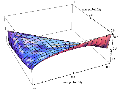
Figure 1: Optimal weight $w^{+}$ versus $\underline{\ddot{P}}\left(\left\{0\right\}\right)$ and $\overline{\ddot{P}}\left(\left\{0\right\}\right)$, the lowest and highest of the plausible probabilities to be combined (10), labeled here as “min. probability” and “max. probability,” respectively. The combination probability is $P^{+}\left(0\right)=w^{+}\underline{\ddot{P}}\left(0\right)+\left(1-w^{+}\right)\overline{\ddot{P}}\left(0\right)$ according to Corollary 1.

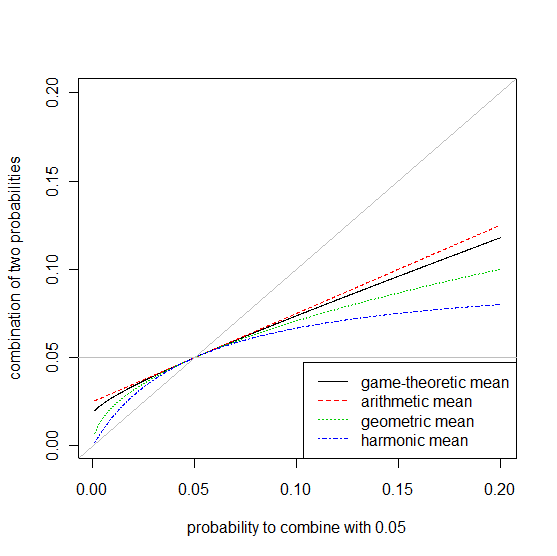
Figure 2: Three equal-weight averages of probabilities and the game-theoretic combination of two probabilities based on Corollary 1. The two probabilities that are combined are drawn in solid gray.

By eq. (5), $37\%\dot{\leq}w^{+}\dot{\leq}63\%$, implying that $P^{+}\left(\left\{0\right\}\right)$ is close to the arithmetic mean $\left[\underline{\ddot{P}}\left(\left\{0\right\}\right)+\overline{\ddot{P}}\left(\left\{0\right\}\right)\right]/2$, as Shulman and Feder (2004) observed in a coding context. Fig. 1 plots $w^{+}$ versus $\underline{\ddot{P}}\left(\left\{0\right\}\right)$ and $\overline{\ddot{P}}\left(\left\{0\right\}\right)$, and Fig. 2 compares the resulting $P^{+}\left(\left\{0\right\}\right)$ to the arithmetic mean, the geometric mean, and the harmonic mean of $\underline{\ddot{P}}\left(\left\{0\right\}\right)$ and $\overline{\ddot{P}}\left(\left\{0\right\}\right)$.

The next result is important for multiple hypothesis testing (§3) and, more generally, for combining probabilities of independent events rather than entire distributions.

Corollary 2.

Let $\xi=\left\langle\xi_{1},\dots,\xi_{N}\right\rangle$, where $\xi_{j}$ is a Bernoulli random variable and $\xi_{j}$ is independent of $\xi_{J}$ for all $j,J=1,\dots N$. (The Bernoulli distributions need not be identical: in general, each has a different probability $\ddot{P}\left(\xi_{i}=0\right)$ of failure. Every $\ddot{P}\in\ddot{\mathcal{P}}$ has a one-to-one correspondence to a tuple $\left\langle\ddot{P}\left(\xi_{1}=0\right),\dots,\ddot{P}\left(\xi_{N}=0\right)\right\rangle$.) Assuming $\dot{\mathcal{P}}\cap\ddot{\mathcal{P}}$ is nonempty and finite, let $\ddot{P}_{i}$ denote the $i$th of the $\nu$ members of $\operatorname{ext}\left(\dot{\mathcal{P}}\cap\ddot{\mathcal{P}}\right)=\left\{\ddot{P}_{1},\dots,\ddot{P}_{\nu}\right\}$. If the constraints are in the form of lower and upper probabilities $\underline{P}_{0,1},\dots,\underline{P}_{0,N}$ and $\overline{P}_{0,1},\dots,\overline{P}_{0,N}$ such that

$$\dot{\mathcal{P}}=\left\{\dot{P}\in\mathcal{P}:\underline{P}{}_{0j}\leq\dot{P}\left(\xi_{j}=0\right)\leq\overline{P}_{0j},j\in\left\{1,\dots,N\right\}\right\},$$ (11)

then the set of combining distributions that satisfy the constraints is

$$\dot{\mathcal{P}}\cap\ddot{\mathcal{P}}=\left\{\ddot{P}\in\ddot{\mathcal{P}}:\underline{P}{}_{0j}\leq\ddot{P}\left(\xi_{j}=0\right)\leq\overline{P}_{0j},j\in\left\{1,\dots,N\right\}\right\}.$$ (12)

Further, $P^{+}=P^{\mathbf{w}_{\operatorname{ext}\left(\dot{\mathcal{P}}\cap\ddot{\mathcal{P}}\right)}}$ is the combination of the distributions in $\ddot{\mathcal{P}}$ with truth constrained by $\dot{\mathcal{P}}$, where

$$\mathbf{w}_{\operatorname{ext}\left(\dot{\mathcal{P}}\cap\ddot{\mathcal{P}}\right)}=\arg\sup_{\left\langle w_{1},\dots,w_{\nu}\right\rangle\in\mathfrak{W}}\sum_{i=1}^{\nu}w_{i}\sum_{j=1}^{N}\sum_{k=0}^{1}\ddot{P}_{i}\left(\xi_{j}=k\right)\log\frac{\ddot{P}_{i}\left(\xi_{j}=k\right)}{P^{\left\langle w_{1},\dots,w_{\nu}\right\rangle}\left(\xi_{j}=k\right)}$$ (13)

with the supremum over $\mathfrak{W}=\left\{\left\langle w_{1}^{\prime},\dots,w_{\nu}^{\prime}\right\rangle\in\left(0,1\right]^{\nu}:\sum_{i=1}^{\nu}w_{i}^{\prime}=1\right\}$.

Proof.

Eq. (12) is obvious from eq. (11). By the independence condition, the chain rule for information divergence (see, e.g., Cover and Thomas, 2006, Theorem 2.5.3) reduces finding the weighting distribution for according to Theorem 2 to finding

$$\mathbf{w}_{\operatorname{ext}\left(\dot{\mathcal{P}}\cap\ddot{\mathcal{P}}\right)}=\arg\sup_{\left\langle w_{1},\dots,w_{\nu}\right\rangle\in\mathfrak{W}}\sum_{i=1}^{\nu}w_{i}\sum_{j=1}^{N}D\left(\ddot{P}_{i}\left(\xi_{j}=\bullet\right)||P^{\left\langle w_{1},\dots,w_{\nu}\right\rangle}\left(\xi_{j}=\bullet\right)\right),$$

which, with eq. (1), yields eq. (13). ∎

3 Distribution combination for statistical inference

Whereas much of the literature focuses on combining priors from experts, Sec. 3.1 instead focuses on combining posteriors. The posterior-inference setting enables the combination not only of Bayesian posterior distributions but also of confidence intervals and p-values encoded as frequentist posterior distributions, as will be explained in Sec. 3.2.

3.1 Combining posterior distributions and probabilities

In the context of posterior statistical inference, $\xi$ represents a random parameter. Further, all distributions in $\dot{\mathcal{P}}$, the set of plausible distributions of $\xi$, and $\ddot{\mathcal{P}}$, the set of combining distributions of $\xi$, are posterior with respect to the same data set $x$. All distributions in $\dot{\mathcal{P}}$ and all Bayesian posteriors in $\ddot{\mathcal{P}}$ are conditional on $X=x$, where, for any such posterior, the distribution of $X$ depends on the random value of the parameter drawn from some prior. $\ddot{\mathcal{P}}$ may also contain non-Bayesian posteriors such as a confidence posterior or a distribution derived from a confidence posterior (§3.2).

Accordingly, the information divergence $D\left(P||Q\right)$ becomes the amount of information that would be gained by replacing any posterior $Q$ with the true posterior $P$. That interpretation leads to viewing $D\left(P^{\prime}||P^{\prime\prime}\rightsquigarrow Q\right)$ as the amount of information gained for statistical inference by using some posterior $Q\in\mathcal{P}$ rather than a given posterior $P^{\prime\prime}\in\ddot{\mathcal{P}}$ when the plausible posterior is $P^{\prime}\in\dot{\mathcal{P}}$. Thus, $D\left(P^{\prime}||P^{\prime\prime}\rightsquigarrow Q\right)$ defines the inferential gain of $Q$ relative to $P^{\prime\prime}$ given $P^{\prime}$ (Bickel, 2011a, c).

The posterior distributions are combined according to Sec. 2.2, using Theorem 1 whenever possible. If $\dot{\mathcal{P}}$ represents the uncertainty around a Bayesian posterior $\dot{P}\in\dot{\mathcal{P}}$, as in Gajdos et al. (2004) and Bickel (2011c), then $\dot{P}$ is included in $\ddot{\mathcal{P}}$ as one of the distributions to combine. The resulting combination $P^{+}$ is then used to minimize expected loss in order to optimize actions such as point, interval, and function estimators and predictors.

In model selection and hypothesis testing, $\xi$ has 0 or 1 as its realized value, with $\xi=0$ if a reduced model or null hypothesis is true or $\xi=1$ if a full model or alternative hypothesis is true. Corollary 1 applies to this problem with $\dot{\mathcal{P}}_{0}$ as the set of feasible null hypothesis posterior probabilities and $\ddot{\mathcal{P}}_{0}=\left\{\ddot{P}_{1}\left(\left\{0\right\}\right),...,\ddot{P}_{c}\left(\left\{0\right\}\right)\right\}$ as the set of null hypothesis posterior probabilities to be combined, where $\ddot{P}_{i}\left(\left\{0\right\}\right)=\ddot{P}_{i}\left(\xi=0\right)$ is the $i$th posterior probability that the null hypothesis is true. Thus, the combination posterior probability that the null hypothesis is true is

$$P^{+}\left(\xi=0\right)=w^{+}\underline{\ddot{P}}\left(\xi=0\right)+\left(1-w^{+}\right)\overline{\ddot{P}}\left(\xi=0\right).$$ (14)

Here, $\underline{\ddot{P}}\left(\xi=0\right)=\underline{\ddot{P}}\left(0\right)$ and $\overline{\ddot{P}}\left(\xi=0\right)=\overline{\ddot{P}}\left(0\right)$ are respectively the lowest and highest null hypothesis posterior probabilities that are in $\dot{\mathcal{P}}_{0}\cap\ddot{\mathcal{P}}_{0}$, presently assumed to have at least one member, and $w^{+}$ is determined by eq. (10). The same idea applies to multiple hypothesis testing, as will be seen in Sec. 4.

3.2 Combining frequentist posteriors

3.2.1 Confidence posteriors

As mentioned in Sec. 3.2, the set $\ddot{\mathcal{P}}$ of posterior combining distributions can include those representing confidence intervals and p-values. To emphasize their comparability to Bayesian posterior distributions, these frequentist distributions are called “confidence posterior distributions” (Bickel, 2011b), also known as “confidence distributions” (see, e.g., Schweder and Hjort, 2002).

Briefly, a confidence posterior distribution that corresponds to a set of nested confidence intervals evaluated for the observed data is defined as the probability distribution according to which the posterior probability that the interest parameter lies within a confidence interval is equal to the confidence level of the interval. For example, if a 95% confidence interval for a real parameter is $\left[-2.2,1.7\right]$, then there is a 95% posterior probability that the parameter is between $-2.2$ and $1.7$ according to the confidence posterior. The same confidence posterior for the data also assigns posterior probability to parameter intervals of interest according to the confidence levels of the matching confidence intervals, e.g., Bickel (2011d) considered a one-sided p-value as the posterior probability that the population mean is in $\left(-\infty,0\right)$ rather than $\left[0,\infty\right)$. Efron and Tibshirani (1998) and Polansky (2007) considered exact confidence posterior probabilities of intervals or other regions specified before observing the data as ideal cases of “attained confidence levels” and “observed confidence levels,” respectively.

Bickel (2011b, d) proposed taking actions that minimize expected loss with respect to a confidence posterior distribution. Since that distribution is a Kolmogorov probability distribution of the parameter of interest, such actions comply with most axiomatic systems usually considered Bayesian, e.g., the systems of von Neumann and Morgenstern (1953) and Savage (1954). A human or artificial intelligent agent that bets and makes other decisions in accordance with minimizing expected loss with respect to a confidence posterior corresponds to equating the confidence level of a confidence interval with the agent’s level of belief that the parameter value lies in the interval (Bickel, 2011b).

The decision-theoretic framework makes confidence posteriors suitable as members of $\ddot{\mathcal{P}}$, the set of combining distributions, according to the methodology of Sec. 2. They can be combined to not only with each other, but also with other parameter distributions such as Bayesian posteriors based on proper or improper priors. The same applies to a probability distribution of a function of a parameter drawn from a confidence posterior. Such posteriors have been used to equate posterior probabilities of simple null hypotheses with two-sided p-values (van Berkum et al., 1996; Bickel, 2011e, a, c). For terminological economy, these posteriors will now be called “confidence posteriors.”

To approximate Bayesian model averaging, Good (1958) recommended a weighted harmonic mean of p-values computed from the same data, provided that they range from $10^{-3}$ to $0.2$, the limits used in Fig. 2. Since the one-sided or two-sided p-values are posterior probabilities of the null hypothesis derived from different confidence posteriors, eqs. (10) and (14) can be applied with $\underline{\ddot{P}}\left(\xi=0\right)$ and $\overline{\ddot{P}}\left(\xi=0\right)$ as the lowest and highest p-values that are plausible as null hypothesis probabilities, i.e., that are in $\dot{\mathcal{P}}_{0}$. The resulting combination p-value differs from that of Good (1958) in two respects: the mean is arithmetic (14) rather than harmonic and, even more important, the weights are optimal for the game (10) rather than subjective. The use of optimal weights leads to preparing for the worst case by averaging only the two most extreme p-values rather than all of them.

Example 2.

Given a small sample of data drawn from a distribution that might be approximately normal, let $p^{\left(1\right)}$ and $p^{\left(2\right)}$ denote the two-sided p-values according to the t-test and the Wilcoxon signed-rank test, respectively; $p^{\left(1\right)}<p^{\left(2\right)}$. Under conditions often applicable to simple (point) hypothesis testing with a diffuse alternative hypothesis (Sellke et al., 2001), the plausible set of posterior probabilities of the null hypothesis is $\dot{\mathcal{P}}_{0}=\left[\underline{\dot{P}}_{0},1\right]$ with lower bound

$$\underline{\dot{P}}_{0}=\left(1+\left(\frac{1-\underline{\dot{P}}_{0}^{\operatorname{prior}}}{\underline{\dot{P}}_{0}^{\operatorname{prior}}ep^{\left(2\right)}\left(x\right)\log\left[1/p^{\left(2\right)}\left(x\right)\right]}\right)\right)^{-1}\wedge\underline{\dot{P}}_{0}^{\operatorname{prior}},$$

where $\wedge$ is the minimum operator, and $\underline{\dot{P}}_{0}^{\operatorname{prior}}$ is the lowest plausible prior probability that the null hypothesis is true (Bickel, 2011c). Then the combined p-value $P^{+}\left(\left\{0\right\}\right)$ is $\underline{\dot{P}}_{0}$ if $p^{\left(2\right)}<\underline{\dot{P}}_{0}$, $p^{\left(2\right)}$ if $p^{\left(1\right)}<\underline{\dot{P}}_{0}\leq p^{\left(2\right)}$, and, according to Corollary 1, the weighted arithmetic mean $w^{+}p^{\left(1\right)}+\left(1-w^{+}\right)p^{\left(2\right)}$ if $p^{\left(1\right)}\geq\underline{\dot{P}}_{0}$ with the weights $w^{+}$ and $\left(1-w^{+}\right)$ fixed by eq. (10). Of the three cases, the third yields a combined p-value that differs from the blended posterior probability suggested in Bickel (2011a). $\operatorname{\blacktriangle}$

When $\ddot{\mathcal{P}}$ consists of a single confidence posterior $\ddot{P}$, the resulting $P^{+}$, degenerate as a “combination” of a single distribution, is better viewed as a solution to the problem of blending frequentist inference with constraints encoded as the Bayesian posteriors that constitute $\dot{\mathcal{P}}$. That solution in general differs from the minimax-type solutions considered (Bickel, 2011a, c). Under $\ddot{P}\in\dot{\mathcal{P}}$ and the convexity of $\dot{\mathcal{P}}$, they lead to the $P$ that minimizes the information divergence $D\left(P||\ddot{P}\right)$, which is dual to the $Q$ that minimizes $D\left(\ddot{P}||Q\right)$, the information divergence that is minimized (15) when maximizing eq. (6) according to the game introduced in Sec. 2.2.

3.2.2 Multiple comparison procedures

The distribution-combination theory is now applied to adjustments for multiple comparisons by formalizing the observation that p-values are often adjusted to the extent of prior belief in the null hypothesis. That is, multiple comparison procedures (MCPs) designed to control error rates are “most likely to be used, if at all, when most of the individual null hypotheses are essentially correct” (Cox, 2006, p.88). A first-order formalization would take the p-value adjusted according to an MCP as the posterior probability of the null hypothesis. To the extent that the knowledge or opinion of the agent is such that its decisions would be made to minimize the expected loss with respect to that posterior distribution, the use of the MCP is warranted. In this interpretation, combining p-values across different MCPs is equivalent to combining the posterior distributions that represent the corresponding opinions.

Example 3.

The Bonferroni procedure controls the family-wise error rate, the probability that one or more true null hypotheses will be rejected, at any level $\alpha\in\left[0,1\right]$. That is accomplished on the basis of p-values $p_{1},\dots,p_{N}$ by rejecting the $i$th of $N$ null hypotheses if the adjusted p-value $Np_{i}\wedge 1$ is less than $\alpha$. Thus, the posterior probabilities generated by the Bonferroni procedure are appropriate only when the prior probability of each null hypothesis is inversely proportional to the number of tests. As Westfall et al. (1997) pointed out, the “Bonferroni method is based upon the implicit presumption of a moderate degree of belief in the event” that all null hypotheses under consideration are true and that the prior truth values of the hypotheses are approximately independent.

Accordingly, the Bonferroni method is widely used to analyze genome-wide association data, largely because only an extremely small fraction $\pi_{1}$ of the hundreds of thousands of markers tested are thought to be associated with the trait of interest. Wellcome Trust Case Control Consortium (2007) guessed $10^{-6}\leq\pi_{1}\leq 10^{-4}$, interpreting $\pi_{1}$ as the prior probability of association between a given marker and the trait. The corresponding range of posterior probabilities and Bayes factors such as those of Wellcome Trust Case Control Consortium (2007) would define $\dot{\mathcal{P}}$ for ruling out MCPs that yield implausible results (Theorem 2). (On the other hand, some evidence that $\pi_{1}\geq 10^{-4}$ is now available in preliminary estimates (Yang and Bickel, 2010) and in indications that thousands of small-effect SNPs may be associated with any particular disease (Gibson, 2010; Park et al., 2010).) $\operatorname{\blacktriangle}$

By assuming adjusted p-values are equal to independent posterior probabilities of the null hypotheses, the methodology of Corollary 2 can combine the results of various MCPs.

4 Large-scale case study

Using microarray technology, Alba et al. (2005) measured the levels of tomato gene expression for 13,440 genes at three days after the breaker stage of ripening, but one or more measurements were missing for 7337 genes. The data available across all $n=6$ biological replicates for $N=6103$ of the genes illustrate the methodology of Secs. 2 and 3.

For $j=1,\dots,N$, the logarithms of the measured ratios of mutant expression to wild-type expression in the $j$th gene were modeled as realizations of a normal variate and are denoted by the $n$-tuple $x_{j}$. Because the mean and variance are unknown, the one-sample t-test was used to test the null hypothesis $\left(\xi_{j}=0\right)$ that the population mean is 0 against the two-sided alternative hypothesis $\left(\xi_{j}=1\right)$ that there is differential expression of the $j$th gene between mutant and wild type, i.e., that the mutation affects the expression of gene $j$.

The posterior probability of a null hypothesis conditional on the p-value is called its local false discovery rate (LFDR) (Efron et al., 2001). Three very different methods $\left(i=1,2,3\right)$ of estimating the LFDR were considered. The first two methods are based on fitting a histogram of transformed p-values that is described by Efron (2007). They differ in that whereas one assumes the p-value has a uniform distribution under the null hypothesis $\left(i=1\right)$, the other estimates the p-value null distribution by maximizing a truncated likelihood function $\left(i=2\right)$. Each method has its own advantages (§1). The distributions are called the theoretical null and the empirical null, respectively. The third method for combination is the q-value (Storey, 2002), here defined according to the algorithm of Benjamini and Hochberg (1995) as the lowest false discovery rate at which a null hypothesis will be rejected $\left(i=3\right)$. While the q-value was not originally intended as an estimator of the LFDR, it is included here since its negative bias as such an estimator (Hong et al., 2009) may have a corrective effect on the positive bias (conservatism) of the first two LFDR estimators.

For this application, $\mathcal{P}$ is the set of all probability distributions on $\left(\left\{0,1\right\}^{N},2^{\left\{0,1\right\}^{N}}\right)$. Corresponding to those three methods, let $\ddot{P}_{1}$, $\ddot{P}_{2}$, and $\ddot{P}_{3}$ denote the members of $\mathcal{P}$ such that the $i$th estimate of the LFDR of the $j$th gene is $\ddot{P}_{i}\left(\xi_{j}=0\right)$. To combine the three methods, $\ddot{\mathcal{P}}=\left\{\ddot{P}_{1},\ddot{P}_{2},\ddot{P}_{3}\right\}$ is taken as the set of $\nu=3$ combining distributions.

For the $j$th gene, $f\left(t\left(x_{j}\right);\theta_{j}\right)$ will represent the probability density of the Student $t$ statistic $t\left(x_{j}\right)$, where $\theta_{j}$ is the reciprocal of the coefficient of variation and, for any $\theta\in\mathbb{R}$, $f\left(\bullet;\theta\right)$ is the probability density function of $\left|T\right|$ when $T$ has the noncentral $t$ distribution of $n-1$ degrees of freedom and noncentrality parameter $\sqrt{n}\theta$. The set $\dot{\mathcal{P}}$ of plausible distributions will be determined on the basis of $\left\{L_{j}\left(\bullet\right)=f\left(t\left(x_{j}\right);\bullet\right):j=1,\dots,N\right\}$, the set of likelihood functions. The plausible distributions are also based on $\underline{\pi}_{0}=80\%$, an assumed lower bound on the proportion of genes that are not differentially expressed. By Bayes’s theorem, the posterior odds of the $j$th null hypothesis is the product of the prior odds, which is the least $\underline{\pi}_{0}/\left(1-\underline{\pi}_{0}\right)$, and the Bayes factor, which must be at least $L_{j}\left(0\right)/\max_{\theta\neq 0}L_{j}\left(\theta\right)$. Thus, for gene $j$, a lower bound $\underline{\Omega}_{j}$ of the posterior odds is the product of the last two quantities, and a lower bound of the LFDR is $\underline{P}\left(\xi_{j}=0\right)=\underline{\Omega}_{j}/\left(1+\underline{\Omega}_{j}\right)$. In the notation of Corollary 2, $\underline{P}_{0,j}=\underline{P}\left(\xi_{j}=0\right)$ and, trivially, $\overline{P}_{0,j}=1$ for all $j=1,\dots,N$. Thus, the plausible set specified by eq. (11) consists of the posterior distributions satisfying the lower bound derived from the likelihood functions and $\underline{\pi}_{0}=80\%$.

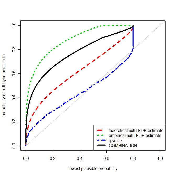
Figure 3: Combination of estimates of local false discovery rates, which are empirical Bayes posterior probabilities that the null hypotheses of equivalent gene expression are true.

The horizontal axis and straight line in Fig. 3 represent $\underline{P}$, and the intermediate, highest, and lowest dashed curves represent $\ddot{P}_{1}$, $\ddot{P}_{2}$, and $\ddot{P}_{3}$, respectively. Since some of the q-values are less than the lower bound $\left(\exists j:\ddot{P}_{3}\left(\xi_{j}=0\right)<\underline{P}\left(\xi_{j}=0\right)\right)$ but all of the other LFDR estimates satisfy the bound $\left(i=1,2;\forall j:\ddot{P}_{i}\left(\xi_{j}=0\right)\geq\underline{P}\left(\xi_{j}=0\right)\right)$, the former are excluded when computing the combined estimates according to eq. (12), in which $\dot{\mathcal{P}}\cap\ddot{\mathcal{P}}=\left\{\ddot{P}_{1},\ddot{P}_{2}\right\}$. Since there are only two distributions, each corresponds to an extreme point, leading to $\operatorname{ext}\left(\dot{\mathcal{P}}\cap\ddot{\mathcal{P}}\right)=\left\{\ddot{P}_{1},\ddot{P}_{2}\right\}$ in eq. (13). Thereby, the combined distribution is numerically found to be the linear combination $P^{+}=w_{1}\ddot{P}_{1}+w_{2}\ddot{P}_{2}$ with $w_{1}=0.43$ and $w_{2}=0.57$. By implication, the game-optimal LFDR estimate for the $j$th gene is $P^{+}\left(\xi_{j}=0\right)=w_{1}\ddot{P}_{1}\left(\xi_{j}=0\right)+w_{2}\ddot{P}_{2}\left(\xi_{j}=0\right)$. Those combined estimates are plotted as the solid curve in Fig. 3.

Appendix A: Remarks

Remark 1.

(Sec. 1) Since formulating the distribution combination problem in terms of a game is unconventional, it is worth noting that game theory laid the foundations of the two dominant schools of statistical decision theory. The maximum-expected-payoff solution of a one-player game (von Neumann and Morgenstern, 1953, Ch. I) led to axiomatic systems that support Bayesian statistics (e.g., Savage, 1954). Likewise, the worst-case (minimax) solutions of certain two-player zero-sum games (von Neumann and Morgenstern, 1953, Ch. III) led to frequentist decision theory (Wald, 1961).

Remark 2.

(Sec. 2.1) The discrete-distribution version of Lemma 1, the main result of the “redundancy-capacity theorem,” was presented by R. G. Gallager in 1974 (Ryabko, 1981, Editor’s Note) and published by Ryabko (1979) and Davisson and Leon-Garcia (1980); cf. Gallager (1979). Cover and Thomas (2006, Theorem 13.1.1), Rissanen (2007, §5.2.1), and Csiszár and Körner (2011, Problem 8.1) provide useful introductions.

Remark 3.

(Sec. 2.2) Previous instances of lexicographically maximizing expected utility with respect to an optimal probability distribution include the use of the least informative prior (Seidenfeld, 2004) and the use of the posterior $P_{2}$ used to maximize $D\left(\dot{P}||P_{1}\rightsquigarrow P_{2}\right)$ in a two-player zero-sum game (Bickel, 2011c). On lexicographic decision making in other contexts, see Levi (1986a, §§5.7, 6.9), Levi (1986b), and Keeney and Raiffa (1993, §3.3.1). Ciesielski (1997, Ch. 4) and Koshy (2004, Ch. 7) provide more formal set-theoretic expositions of lexicographic ordering.

Appendix B: Additional proofs

Proof of Theorem 1

For any $Q\in\mathcal{P}$, eqs. (2) and (6) yield

$$\sup_{\left\langle P^{\prime},P^{\prime\prime}\right\rangle\in\dot{\mathcal{P}}\times\ddot{\mathcal{P}}}^{\preceq}U\left(P^{\prime},Q,P^{\prime\prime}\right) = \sup_{\left\langle P^{\prime},P^{\prime\prime}\right\rangle\in\dot{\mathcal{P}}\times\ddot{\mathcal{P}}}^{\preceq}\left\langle-D\left(P^{\prime}||P^{\prime\prime}\right),D\left(P^{\prime}||Q\rightsquigarrow P^{\prime\prime}\right)\right\rangle$$

$$= \sup_{P^{\prime}\in\dot{\mathcal{P}}\cap\ddot{\mathcal{P}}}^{\preceq}\left\langle-D\left(P^{\prime}||P^{\prime}\right),D\left(P^{\prime}||Q\rightsquigarrow P^{\prime}\right)\right\rangle$$

$$= \sup_{P^{\prime}\in\dot{\mathcal{P}}\cap\ddot{\mathcal{P}}}\left[D\left(P^{\prime}||Q\right)-D\left(P^{\prime}||P^{\prime}\right)\right]=\sup_{P^{\prime}\in\dot{\mathcal{P}}\cap\ddot{\mathcal{P}}}D\left(P^{\prime}||Q\right).$$

Thus, by eqs. (2), (6), (7), and (8),

$$P^{+} = \arg\sup_{Q\in\mathcal{P}}^{\preceq}U\left(\arg\sup_{P^{\prime}\in\dot{\mathcal{P}}\cap\ddot{\mathcal{P}}}D\left(P^{\prime}||Q\right),\arg\sup_{P^{\prime}\in\dot{\mathcal{P}}\cap\ddot{\mathcal{P}}}D\left(P^{\prime}||Q\right),Q\right)$$ (15)

$$= \arg\sup_{Q\in\mathcal{P}}\left(-D\left(\arg\sup_{P^{\prime}\in\dot{\mathcal{P}}\cap\ddot{\mathcal{P}}}D\left(P^{\prime}||Q\right)||Q\right)\right)$$

$$= \arg\inf_{Q\in\mathcal{P}}\sup_{P^{\prime}\in\dot{\mathcal{P}}\cap\ddot{\mathcal{P}}}D\left(P^{\prime}||Q\right).$$

Hence, according to eq. (3), $P^{+}$ is $\widetilde{\dot{\mathcal{P}}\cap\ddot{\mathcal{P}}}$, the centroid of $\dot{\mathcal{P}}\cap\ddot{\mathcal{P}}$. Since $\dot{\mathcal{P}}\cap\ddot{\mathcal{P}}\neq\emptyset$ by assumption, the conditions of Lemma 1 are satisfied.

Proof of Lemma 2

As an immediate consequence of what Nakagawa and Kanaya (1988) label “Theorem (Csiszár)” and “Theorem 1,”

$$\min_{P^{\prime\prime}\in\mathcal{P}}\max_{P^{\prime}\in\mathcal{P}^{\star}}D\left(P^{\prime}||P^{\prime\prime}\right)=C.$$

By definition, the centroid is the solution of that minimax problem (3).

Proof of Theorem 2

Lemma 1 implies that $\widetilde{\operatorname{ext}\left(\dot{\mathcal{P}}\cap\ddot{\mathcal{P}}\right)}$, the centroid of $\operatorname{ext}\left(\dot{\mathcal{P}}\cap\ddot{\mathcal{P}}\right)$, is $P^{W_{\operatorname{ext}\left(\dot{\mathcal{P}}\cap\ddot{\mathcal{P}}\right)}}$. Since, according to the definition of an extreme point and the definition of a centroid (3), it is not possible that there exist a $P^{\prime}\in\operatorname{ext}\left(\dot{\mathcal{P}}\cap\ddot{\mathcal{P}}\right)$ and a $P^{\prime\prime}\in\operatorname{ext}\left(\dot{\mathcal{P}}\cap\ddot{\mathcal{P}}\right)$ such that $D\left(P^{\prime}||\widetilde{\operatorname{ext}\left(\dot{\mathcal{P}}\cap\ddot{\mathcal{P}}\right)}\right)<D\left(P^{\prime\prime}||\widetilde{\operatorname{ext}\left(\dot{\mathcal{P}}\cap\ddot{\mathcal{P}}\right)}\right)$, it follows that

$$D\left(P^{\star}||P^{W_{\operatorname{ext}\left(\dot{\mathcal{P}}\cap\ddot{\mathcal{P}}\right)}}\right)=\max_{P^{\prime}\in\operatorname{ext}\left(\dot{\mathcal{P}}\cap\ddot{\mathcal{P}}\right)}D\left(P^{\prime}||P^{W_{\operatorname{ext}\left(\dot{\mathcal{P}}\cap\ddot{\mathcal{P}}\right)}}\right)$$

for all $P^{\star}\in\operatorname{ext}\left(\dot{\mathcal{P}}\cap\ddot{\mathcal{P}}\right)$. According to Lemma 2, $P^{W_{\operatorname{ext}\left(\dot{\mathcal{P}}\cap\ddot{\mathcal{P}}\right)}}$ is $\widetilde{\dot{\mathcal{P}}\cap\ddot{\mathcal{P}}}$, the centroid of $\dot{\mathcal{P}}\cap\ddot{\mathcal{P}}$. That centroid is $P^{+}$ by Theorem 1.

References

- Abbas (2009) Abbas, A. E., Mar. 2009. A Kullback-Leibler View of Linear and Log-Linear Pools. Decision Analysis 6, 25–37.
- Alba et al. (2005) Alba, R., Payton, P., Fei, Z., McQuinn, R., Debbie, P., Martin, G. B., Tanksley, S. D., Giovannoni, J. J., 2005. Transcriptome and selected metabolite analyses reveal multiple points of ethylene control during tomato fruit development. Plant Cell 17, 2954–2965.
- Barndorff-Nielsen (1995) Barndorff-Nielsen, O. E., 1995. Diversity of evidence and birnbaum’s theorem. Scandinavian Journal of Statistics 22, 513–515.
- Benjamini and Hochberg (1995) Benjamini, Y., Hochberg, Y., 1995. Controlling the false discovery rate: A practical and powerful approach to multiple testing. Journal of the Royal Statistical Society B 57, 289–300.
- Berger (1985) Berger, J. O., 1985. Statistical Decision Theory and Bayesian Analysis. Springer, New York.
- Bickel (2011a) Bickel, D. R., 2011a. Blending Bayesian and frequentist methods according to the precision of prior information with an application to hypothesis testing. Technical Report, Ottawa Institute of Systems Biology, arXiv:1107.2353.
- Bickel (2011b) Bickel, D. R., 2011b. Coherent frequentism: A decision theory based on confidence sets. To appear in Communications in Statistics - Theory and Methods (accepted 22 November 2010); 2009 preprint available from arXiv:0907.0139.
- Bickel (2011c) Bickel, D. R., 2011c. Controlling the degree of caution in statistical inference with the Bayesian and frequentist approaches as opposite extremes. Technical Report, Ottawa Institute of Systems Biology, arXiv:1109.5278.
- Bickel (2011d) Bickel, D. R., 2011d. Estimating the null distribution to adjust observed confidence levels for genome-scale screening. Biometrics 67, 363–370.
- Bickel (2011e) Bickel, D. R., 2011e. Small-scale inference: Empirical Bayes and confidence methods for as few as a single comparison. Technical Report, Ottawa Institute of Systems Biology, arXiv:1104.0341.
- Ciesielski (1997) Ciesielski, K., 1997. Set Theory for the Working Mathematician. Cambridge University Press, Cambridge.
- Clemen and Winkler (1999) Clemen, R. T., Winkler, R. L., 1999. Combining probability distributions from experts in risk analysis. Risk Analysis 19, 187–203.
- Cooke (1991) Cooke, R. M., 1991. Experts in Uncertainty: Opinion and Subjective Probability in Science. Oxford University Press.
- Cover and Thomas (2006) Cover, T., Thomas, J., 2006. Elements of Information Theory. John Wiley and Sons, New York.
- Cox (2006) Cox, D. R., 2006. Principles of Statistical Inference. Cambridge University Press, Cambridge.
- Csiszár and Körner (2011) Csiszár, I., Körner, J., 2011. Information Theory: Coding Theorems for Discrete Memoryless Systems. Cambridge University Press, Cambridge.
- Davisson and Leon-Garcia (1980) Davisson, L., Leon-Garcia, a., Mar. 1980. A source matching approach to finding minimax codes. IEEE Transactions on Information Theory 26, 166–174.
- Efron (2007) Efron, B., 2007. Size, power and false discovery rates. Annals of Statistics 35, 1351–1377.
- Efron (2010) Efron, B., 2010. Large-Scale Inference: Empirical Bayes Methods for Estimation, Testing, and Prediction. Cambridge University Press.
- Efron and Tibshirani (1998) Efron, B., Tibshirani, R., 1998. The problem of regions. Annals of Statistics 26, 1687–1718.
- Efron et al. (2001) Efron, B., Tibshirani, R., Storey, J. D., Tusher, V., 2001. Empirical Bayes analysis of a microarray experiment. J. Am. Stat. Assoc. 96, 1151–1160.
- Gajdos et al. (2004) Gajdos, T., Tallon, J. M., Vergnaud, J. C., SEP 2004 2004. Decision making with imprecise probabilistic information. Journal of Mathematical Economics 40, 647–681.
- Gallager (1979) Gallager, R. G., 1979. Source coding with side information and universal coding. Technical Report LIDS-P-937, Laboratory for Information Decision Systems, MIT.
- Genest and Zidek (1986) Genest, C., Zidek, J. V., 1986. Combining Probability Distributions: A Critique and an Annotated Bibliography. Statistical Science 1, 114–135.
- Gibson (2010) Gibson, G., Jul. 2010. Hints of hidden heritability in GWAS. Nature Genetics 42, 558–60.
- Good (1984) Good, I., 1984. A Bayesian interpretation of ancillarity. Journal of Statistical Computation and Simulation 19 (4), 302–308.
- Good (1958) Good, I. J., 1958. Significance tests in parallel and in series. Journal of the American Statistical Association 53, 799–813.
- Grünwald and Philip Dawid (2004) Grünwald, P., Philip Dawid, A., 2004. Game theory, maximum entropy, minimum discrepancy and robust Bayesian decision theory. Annals of Statistics 32, 1367–1433.
- Haussler (1997) Haussler, D., 1997. A general minimax result for relative entropy. IEEE Transactions on Information Theory 43, 1276 – 1280.
- Hong et al. (2009) Hong, W.-J., Tibshirani, R., Chu, G., 2009. Local false discovery rate facilitates comparison of different microarray experiments. NUCLEIC ACIDS RESEARCH 37 (22), 7483–7497.
- Keeney and Raiffa (1993) Keeney, R. L., Raiffa, H., 1993. Decisions with Multiple Objectives: Preferences and Value Tradeoffs. Cambridge University Press, Cambridge.
- Koshy (2004) Koshy, T., 2004. Discrete mathematics with applications. Academic Press.
- Kracík (2011) Kracík, J., 2011. Combining marginal probability distributions via minimization of weighted sum of Kullback-Leibler divergences. International Journal of Approximate Reasoning 52, 659–671.
- Levi (1986a) Levi, I., 1986a. Hard Choices: Decision Making under Unresolved Conflict. Cambridge University Press, Cambridge.
- Levi (1986b) Levi, I., 1986b. The paradoxes of Allais and Ellsberg. Economics and Philosophy 2, 23–53.
- McConway (1981) McConway, K. J., 1981. Marginalization and linear opinion pools. Journal of the American Statistical Association 76, 410–414.
- Nakagawa and Kanaya (1988) Nakagawa, K., Kanaya, F., 1988. A new geometric capacity characterization of a discrete memoryless channel. IEEE Transactions on Information Theory 34, 318–321.
- Park et al. (2010) Park, J.-H., Wacholder, S., Gail, M. H., Peters, U., Jacobs, K. B., Chanock, S. J., Chatterjee, N., Jul. 2010. Estimation of effect size distribution from genome-wide association studies and implications for future discoveries. Nature Genetics 42, 570–5.
- Pfaffelhuber (1977) Pfaffelhuber, E., 1977. Minimax Information Gain and Minimum Discrimination Principle. In: Csiszár, I., Elias, P. (Eds.), Topics in Information Theory. Vol. 16 of Colloquia Mathematica Societatis János Bolyai. János Bolyai Mathematical Society and North-Holland, pp. 493–519.
- Polansky (2007) Polansky, A. M., 2007. Observed Confidence Levels: Theory and Application. Chapman and Hall, New York.
- Rissanen (2007) Rissanen, J., 2007. Information and Complexity in Statistical Modeling. Springer, New York.
- Ryabko (1979) Ryabko, B., 1979. Encoding of a source with unknown but ordered probabilities. Prob. Pered. Inform. 15, 71–77.
- Ryabko (1981) Ryabko, B., Nov. 1981. Comments on ’A source matching approach to finding minimax codes’ by Davisson, L. D. and Leon-Garcia, A. IEEE Transactions on Information Theory 27, 780–781.
- Savage (1954) Savage, L. J., 1954. The Foundations of Statistics. John Wiley and Sons, New York.
- Schweder and Hjort (2002) Schweder, T., Hjort, N. L., 2002. Confidence and likelihood. Scandinavian Journal of Statistics 29, 309–332.
- Seidenfeld (2004) Seidenfeld, T., 2004. A contrast between two decision rules for use with (convex) sets of probabilities: -maximin versus. Synthese 140, 69–88.
- Sellke et al. (2001) Sellke, T., Bayarri, M. J., Berger, J. O., 2001. Calibration of p values for testing precise null hypotheses. American Statistician 55, 62–71.
- Shulman and Feder (2004) Shulman, N., Feder, M., 2004. The uniform distribution as a universal prior. IEEE Transactions on Information Theory 50, 581–586.
- Storey (2002) Storey, J. D., 2002. A direct approach to false discovery rates. Journal of the Royal Statistical Society. Series B: Statistical Methodology 64, 479–498.
- Toda (1956) Toda, M., May 1956. Information-receiving behavior of man. Psychological Review 63, 204–212.
- Topsøe (2007) Topsøe, F., 2007. Information theory at the service of science. In: Tóth, G. F., Katona, G. O. H., Lovász, L., Pálfy, P. P., Recski, A., Stipsicz, A., Szász, D., Miklós, D., Csiszár, I., Katona, G. O. H., Tardos, G., Wiener, G. (Eds.), Entropy, Search, Complexity. Bolyai Society Mathematical Studies. Springer Berlin Heidelberg, pp. 179–207.
- van Berkum et al. (1996) van Berkum, E., Linssen, H., Overdijk, D., 1996. Inference rules and inferential distributions. Journal of Statistical Planning and Inference 49, 305–317.
- von Neumann and Morgenstern (1953) von Neumann, J., Morgenstern, O., 1953. Theory of Games and Economic Behavior. Princeton University Press, Princeton.
- Wald (1961) Wald, A., 1961. Statistical Decision Functions. John Wiley and Sons, New York.
- Wellcome Trust Case Control Consortium (2007) Wellcome Trust Case Control Consortium, 2007. Genome-wide association study of 14,000 cases of seven common diseases and 3,000 shared controls. Nature 447, 661–678.
- Westfall et al. (1997) Westfall, P. H., Johnson, W. O., Utts, J. M., 1997. A Bayesian perspective on the Bonferroni adjustment. Biometrika 84, 419–427.
- Yang and Bickel (2010) Yang, Y., Bickel, D. R., 2010. Minimum description length and empirical Bayes methods of identifying SNPs associated with disease. Technical Report, Ottawa Institute of Systems Biology, COBRA Preprint Series, Article 74, biostats.bepress.com/cobra/ps/art74.