Production of interstellar hydrogen peroxide (H₂O₂) on the surface of dust grains

Abstract

Context. The formation of water on the dust grains in the interstellar medium may proceed with hydrogen peroxide (H₂O₂) as an intermediate. Recently gas-phase H₂O₂ has been detected in $\rho$ Oph A with an abundance of $\sim$10^-10 relative to H₂.

Aims. We aim to reproduce the observed abundance of H₂O₂ and other species detected in $\rho$ Oph A quantitatively.

Methods. We make use of a chemical network which includes gas phase reactions as well as processes on the grains; desorption from the grain surface through chemical reaction is also included. We run the model for a range of physical parameters.

Results. The abundance of H₂O₂ can be best reproduced at $\sim$6$\times$10⁵ yr, which is close to the dynamical age of $\rho$ Oph A. The abundances of other species such as H₂CO, CH₃OH, and O₂ can be reasonably reproduced also at this time. In the early time the gas-phase abundance of H₂O₂ can be much higher than the current detected value. We predict a gas phase abundance of O₂H at the same order of magnitude as H₂O₂, and an abundance of the order of 10^-8 for gas phase water. A few other species of interest are also discussed.

Conclusions. We demonstrate that H₂O₂ can be produced on the dust grains and released into the gas phase through non-thermal desorption via surface exothermic reactions. The H₂O₂ molecule on the grain is an important intermediate in the formation of water. The fact that H₂O₂ is over-produced in the gas phase for a range of physical conditions suggests that its destruction channel in the current gas phase network may be incomplete.

1 Introduction

Oxygen is the most abundant “metal” element in the cosmos (Savage & Sembach 1996; Asplund et al. 2009). In the cold dense interstellar clouds, gas phase chemical models predict that oxygen mainly resides in CO and O₂ molecules (Herbst & Leung 1989; Millar & Herbst 1990; Wakelam et al. 2006). However, although CO is ubiquitously distributed in the interstellar medium, O₂ is not. The latter is only detected very recently in $\rho$ Oph A at a low abundance (relative to molecular hydrogen) of 5$\times$10^-8 (Larsson et al. 2007), and in Orion at an abundance of (0.3 – 7)$\times$10^-6 (Goldsmith et al. 2011). On the other hand, the observed water (gas or ice) abundance can be as high as 10^-4 (van Dishoeck 2004). Thus it seems that water, instead of O₂, is a main reservoir of oxygen in addition to CO. When only gas phase chemistry is included, the H₂O abundance can be of the order 10^-7 at most (see, for example, Bergin et al. 2000; Roberts & Herbst 2002) for typical dark cloud conditions. The fact that O₂ is over-produced and H₂O is under-produced in gas phase chemistry suggests that adsorption onto the grain surfaces and the reactions on the surfaces may play an important role.

On the grain surface, H₂O can form through successive additions of hydrogen atoms to an oxygen atom:

$${\rm H}+{\rm O} \rightarrow{\rm OH},$$ (1)

$${\rm H}+{\rm OH} \rightarrow{\rm H}_{2}{\rm O},$$ (2)

both of which are barrierless (Allen & Robinson 1977). It can also form via hydrogen addition to molecular oxygen:

$${\rm H}+{\rm O}_{2} \rightarrow{\rm O}_{2}{\rm H},$$ (3)

$${\rm H}+{\rm O}_{2}{\rm H} \rightarrow{\rm H}_{2}{\rm O}_{2},$$ (4)

$${\rm H}+{\rm H}_{2}{\rm O}_{2} \rightarrow{\rm H}_{2}{\rm O}+{\rm OH}.$$ (5)

Reaction (3) was assumed to have an activation barrier of 1200 K in Tielens & Hagen (1982). However, based on experimental results, Cuppen et al. (2010) recently concluded that it is barrierless. Other possible formation pathways of water include the reaction between H₂ and OH and the route with O₃ as an intermediate (Tielens & Hagen 1982).

In the second route described above (equations (3 – 5)), hydrogen peroxide (HOOH, also written as H₂O₂, which is adopted in this paper) appears as an intermediate product. Thus if this route is indeed important, a significant amount of H₂O₂ might form on the grain, and its gas phase counterpart could also be detectable if effective desorption mechanisms exist.

In the current mainstream gas phase reaction networks for astrochemistry, H₂O₂ is not efficiently formed in the gas phase. For example, in the 2009 version of the OSU network, the only two reactions leading to the formation of H₂O₂ are

$${\rm H}_{2}+{\rm O}_{2}{\rm H} \rightarrow{\rm H}_{2}{\rm O}_{2}+{\rm H},$$

$${\rm OH}+{\rm OH} \rightarrow{\rm H}_{2}{\rm O}_{2}+h\nu.$$

The first one has a large activation barrier of 10⁴ K, rendering it inactive at low temperatures. H₂O₂ is mainly consumed by

$${\rm H}_{2}{\rm O}_{2}+h\nu \rightarrow{\rm OH}+{\rm OH},$$

$${\rm OH}+{\rm H}_{2}{\rm O}_{2} \rightarrow{\rm H}_{2}{\rm O}+{\rm O}_{2}{\rm H},$$

the first of which is dissociation by cosmic-ray induced radiation. Other destruction channels by reacting with H and O are ineffective due to large activation barriers. At a temperature of 10 K and an H₂ density of 10⁴ cm^-3, the steady-state abundance of H₂O₂ can be approximated by

$$X({\rm H}_{2}{\rm O}_{2})\simeq 10^{3}X^{2}({\rm OH})\simeq 5\times 10^{-12}.$$

At a higher density, the abundance of H₂O₂ will be even less because OH is less abundant in this case. With the UMIST RATE06 network the abundance of H₂O₂ is essentially zero (Woodall et al. 2007).

Thus if a substantial amount of H₂O₂ can be detected in the interstellar medium, then it must have been synthesized on the dust grains, rather than in the gas phase; this would also provide information and constraints on the formation route of H₂O.

And it was indeed recently detected (for the first time) in the $\rho$ Oph A cloud by Bergman et al. (2011b), at an abundance of $\sim$10^-10, which is well above what would be predicted by the gas phase chemistry, indicating that chemical processes on the grains are responsible for this detection. Why this molecule has not been detected in the past seems to be a puzzle and will be discussed later.

In the present work we aim at modeling the gas phase abundance of H₂O₂ at a physical condition relevant to $\rho$ Oph A, to demonstrate whether the grain chemistry is able to explain its observed abundance. The model is also required to give consistent abundances for other species detected earlier in this region. Also, ice and gas-phase abundance predictions for previously undetected species will be done.

The remaining part of this paper is organized as follows. In section 2 we describe the chemical model being used in this work. In section 3 we present the results of our modeling. The conclusions are in section 4. Appendix A contains an explanation to a spike-like feature in the evolution curves of some species. The surface reaction network we use is listed in appendix B, and the enthalpies of the surface species which are needed in the chemical desorption mechanism (see section 2) are listed in appendix C.

2 Chemical model

For the gas phase chemistry, we make use of a subset of the UMIST RATE06 network (Woodall et al. 2007). Species containing Fe, Na, Mg, Cl are excluded. In total 284 gas phase species and 3075 gas phase reactions are included. The cosmic-ray ionization rate is taken to be the canonical value of 1.36$\times 10^{-17}$ s^-1 (Woodall et al. 2007).

The surface chemical network is a combination of a selection of the reactions in Allen & Robinson (1977), Tielens & Hagen (1982) and Hasegawa et al. (1992), with the rates of a few reactions updated according to the recent experimental results and/or theoretical calculations. In total 56 surface species and 151 surface reactions are included (see appendix B).

The binding energies of the surface species are either taken from Hasegawa & Herbst (1993), or estimated from the value of a similar species in a way similar to Garrod et al. (2008). These values are applicable to bare grains, i.e., grains without an ice mantle. A grain will be covered by ice (typically water) as adsorption and reaction proceeds, thus these values are not always appropriate. Ideally, they should be varied according to the real-time composition of the grain. The water ice mantle mainly affects the binding energies of species with a hydrogen bond, such as OH and H₂O. The effect of this should be minor for our purpose, because most of the reactions involving a species with a hydrogen bond are primarily mediated by another reaction partner which does not have a hydrogen bond.

The barriers against surface diffusion are taken to be a fixed fraction of the binding energies. A range of values have been used for this fraction in the past, from 0.3 (Hasegawa et al. 1992) through 0.5 (Garrod et al. 2008) to 0.77 (Ruffle & Herbst 2000). We use a value of 0.77, based on the analysis of Katz et al. (1999). Because our model is mainly for a relatively high temperature ($\sim$20 K) in comparison with most of the previous models (predominantly for a temperature of $\sim$10 K), a low diffusion barrier for the surface species would lead to an unrealistic ice mantle composition. The effect of changing this parameter is discussed later. We allow H and H₂ on a dust grain to migrate through quantum tunneling or thermal hopping, depending on which is faster; all the heavier species are only allowed to move by thermal hopping. The quantum tunneling and thermal hopping rates are calculated using the formulation of Hasegawa et al. (1992). For calculation of the quantum tunneling rates, we use a barrier width of 1 $\AA$. The exact value of this width depends on the composition and structure of the surface, which has not been fully quantified.

About the activation barrier of reaction (3), as there is a big discrepancy between the value adopted in the past and the value proposed recently based on experiments (Cuppen et al. 2010), we adopt an intermediate value of 600 K. However, the effect of varying this parameter is also tested during the modeling, and will be discussed later. Reaction (5) has a barrier of 1400 K in Tielens & Hagen (1982), while in Cuppen et al. (2010) this reaction is barrierless. We choose to adopt the latter result in this case, because too high a barrier for it would result in building-up too much of H₂O₂ on the grain surface.

Surface reactions with an activation barrier are allowed to proceed thermally or through quantum tunneling, depending on whichever is faster. The formula used to calculate the rates is also the same as in Hasegawa et al. (1992), and the reaction barriers are assumed to have a width of 1 $\AA$, although different values are possible (Garrod & Pauly 2011).

The reaction rate of a two-body surface reaction

$${\rm A+B\rightarrow C+\cdots}$$

is

$$[k_{\rm diff}({\rm A})+k_{\rm diff}({\rm B})]N({\rm A})N({\rm B)}/N_{\rm S},$$

if ${\rm A\neq B}$. Here $N_{\rm S}$ is the number of reaction sites of a grain, $k_{\rm diff}({\rm A})$ and $k_{\rm diff}(B)$ are the diffusion rates of A and B, and $N({\rm A})$ and $N({\rm B})$ are the number of species A and B on a single grain, respectively. If ${\rm A=B}$, then the reaction rate should be

$$k_{\rm diff}(A)N({\rm A})(N({\rm A})-1)/N_{\rm S}.$$

With a number density of reaction sites being 10¹⁵ cm^-2, a dust grain with radius 0.1 $\mu$m has a $N_{\rm S}$ of about 10⁶.

As we are mainly concerned with the gas phase abundances of several species, their desorption mechanism must be treated carefully, especially if they are mainly produced on the grains. Besides the normal thermal desorption, species can also get evaporated episodically when a cosmic-ray hits a grain. This is treated in the same manner as in Hasegawa & Herbst (1993). Furthermore, the non-thermal desorption mechanism via exothermic surface reactions (for brevity we call it “chemical desorption” hereafter) proposed by Garrod et al. (2006) (see also Watson & Salpeter 1972; Garrod et al. 2007; Cazaux et al. 2010) is also included. Here the products of the exothermic reactions on the grain have a probability to be directly ejected into the gas phase. The rate of such a desorption mechanism depends on the exoergicity of the reaction, as well as on the desorption energy of the products. A parameter characterizing the efficiency of this mechanism (the parameter “$a$” in Garrod et al. (2007)) is introduced, which we take to be 0.1. The yield of chemical desorption is directly proportional to this “a” parameter, although it is not well-constrained. The value we adopt here gives a good match to the observational results. See section 3.6 for a further discussion. The exoergicities of these reactions are estimated from the enthalpies of the reactants and products in the same manner as in Allen & Robinson (1977) (their equations (3) and (4)), and the enthalpies of the species involved in these reactions are taken from Binnewies & Milke (1999) or the NIST chemistry web book, or some other sporadic sources (see appendix C).

However, the desorption mechanisms described above alone are not always sufficient to provide enough gas phase abundances for some species, especially at late times. Even if a large amount of a species is produced on the grain and released into the gas phase at early times, later it would be accreted back to the grain surface. If at this later time its production is no longer active (due to the exhaustion of the precursor species), its gas phase abundance cannot be maintained. Dust sputtering (Tielens et al. 1994) and photo-desorption (Öberg et al. 2007) might help to release them to the gas phase, both of which should not be of great importance in a quiet cold dark cloud. Another possible mechanism is that cosmic-ray induced radiation can dissociate the species on the grain, and when the fragments recombine, the products can possibly be ejected into the gas phase directly because of the energy release of the reaction, as described before. We implement this mechanism in the same way as in Ruffle & Herbst (2001a) and Garrod & Pauly (2011) (see also Cuppen & Herbst 2007), namely, the cosmic-ray induced photo-dissociation rates for the surface species are taken to be the same as in the gas phase. Several dissociation branches from Garrod et al. (2008) (their Table 1) are included.

In our model the numbers of all the species on a single grain are solved with the hybrid moment equation (HME) approach (Du & Parise 2011). It has been shown in Du & Parise (2011) that the rate equation method can be inaccurate in some cases, and the HME approach provides a major improvement over the rate equation method. As the HME approach is relatively new, in several cases we also benchmarked our HME results with the exact Monte Carlo method (similar to the one of Vasyunin et al. 2009) as in Du & Parise (2011), and the agreement is satisfactory. It is impractical to run all the models with the Monte Carlo method because the run time would be too long.

At present the layered structure of the grain mantle is not incorporated into our model. Although such a structure might be more realistic, and it is important for retaining some of the ice species, however, it is also possible that the interstellar dust grains may have an amorphous structure, which renders the layered structure an inaccurate description. On the other hand, particles landing on a grain are able to penetrate into the interior by several to tens of layers, as demonstrated by experiments (see, e.g., Ioppolo et al. 2010), thus although a model neglecting the layered structure is not accurate, one which deactivates all the layers below the outermost surface does not reflect the whole reality either. In fact, for the H-addition reactions, whether the layered structure is taken into account or not only plays a minor role in determining the reaction rates in the accretion limit (i.e. when the accretion and evaporation processes are much slower than the reactions (Garrod 2008)), because the species involved in these reactions never build up a full layer.

3 Results and discussions

3.1 Modeling $\rho$ Oph A

We have run the chemical model for physical parameters which are appropriate for $\rho$ Oph A, where H₂O₂ is first detected by Bergman et al. (2011b). In Fig. 1 we show the abundances of several species as a function of time. In this model, a temperature of 21 K and a hydrogen density of 6$\times$10⁵ cm^-3 has been assumed, which are determined for $\rho$ Oph A observationally by Bergman et al. (2011a, b). The dust temperature and gas temperature are assumed to be the same. A fixed value of 15 for the visual extinction $A_{\rm V}$ has been adopted. We assume a canonical grain size of 0.1 $\mu$m and a reaction site density of 10¹⁵ cm^-2. The dust-to-gas mass ratio is set to 0.01, and the dust grain material is assumed to have a mass density of 2 g cm^-3. We also assume that the ratio between the diffusion barrier and the binding energy is 0.77, which is at the higher end of the values that have been used in the past, to give a reasonable ice composition. The initial condition is atomic except for H₂. The elemental abundances are the same as in Garrod & Pauly (2011).

The observed abundance of gas phase H₂O₂ is $\sim$10^-10 relative to H₂ (Bergman et al. 2011b). This value is best matched at a time of $\sim$6$\times$10⁵ yr. In the early time, before about 2$\times$10⁵ years, the gas phase H₂O₂ abundance can be as high as $\sim$5$\times$10^-7. At late times the H₂O₂ abundance decreases to a very low value, due to the exhaustion of O₂ on the grain and a full conversion of H₂O₂ into H₂O.

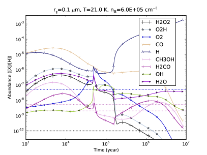
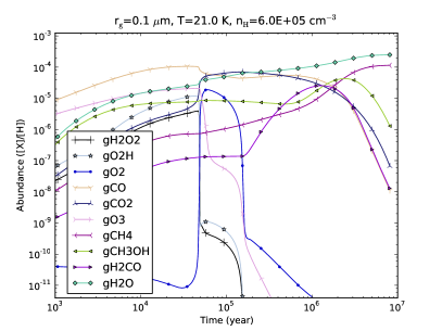
Figure 1: The time evolution of the abundances of selected species. A prefix “g” means a grain surface species (right panel), while a name without a prefix means a gas phase species (left panel). The dotted lines are the observed abundances (relative to H₂) of O₂ (blue), H₂CO (cyan), CH₃OH (magenta), and H₂O₂ (black), respectively, in the $\rho$ Oph A source.

H₂O₂ is mainly formed through reaction (4) on the grain, followed by immediate desorption of the product into the gas phase caused by the reaction heat. About 7% of the produced H₂O₂ are released this way. Its gas phase abundance is determined by the adsorption and chemical desorption processes. The dissociation of gas phase H₂O₂ by cosmic-ray-induced photons is unimportant in consuming it, in comparison with adsorption.

Ioppolo et al. (2008) modeled the abundance of H₂O₂ ice briefly, giving a value of 10^-14 – 10^-10 relative to molecular hydrogen, depending on which energy barriers of several relevant reactions have been used. Our major goal is to model the gas phase H₂O₂ abundance, rather than the H₂O₂ ice. In our model results, the gas phase abundance of H₂O₂ is much higher than its ice counterpart. The H₂O₂ ice does not have a significant abundance in the later stage, being well below the upper limit (5.2% with respect to H₂O ice) given by Boudin et al. (1998), because it is constantly transformed into H₂O by reacting with the accreted H atoms. However, by irradiating thin water ice film with low energy ions, Gomis et al. (2004) found that it is possible to obtain an H₂O₂ to H₂O ratio in the solid phase up to a few percent. This direct processing of the grain mantle by cosmic rays is not included in our model. The production of H₂O₂ inside water ice in an O₂ rich environment triggered by UV radiation (Shi et al. 2011) should also be of little importance here. We notice in Fig. 1 (right panel) that in the early stage (before $\sim$5$\times$10⁴ yr) the H₂O₂ ice can achieve a rather high abundance, $\sim$5$\times$10^-6 relative to H nucleus or $\sim$10% relative to H₂O. During this early period the water formation on the grain mainly proceeds through reaction (5) with H₂O₂ as an intermediate, which is responsible for about half of the final water ice repository on the grain mantle. In the later stage reaction (2) takes over. In the results of Ioppolo et al. (2008) (their Fig. 4) we do not see a similar feature (i.e. a high abundance of H₂O₂ ice in the early stage). In our current model the layered structure of the grain mantle is not taken into account. It is possible that, if such a structure is considered, the inner layers with a relatively high H₂O₂ content might be maintained, which would give a value of a few percent for the H₂O₂ to H₂O ratio in the solid phase.

Methanol (CH₃OH) and formaldehyde (H₂CO) are also detected in the $\rho$ Oph A SM1 core (Bergman et al. 2011a), at an abundance of $\sim$2$\times$10^-9 and $\sim$5$\times$10^-9, respectively. Their abundances are also reproduced very well at a time of $\sim$6$\times$10⁵ yr in our model. At early times, both CH₃OH and H₂CO have a high abundance. Their abundances also have a peak in the period between 2$\times$10⁵ yr to 10⁷ yr. In our current network, CH₃OH is mainly formed on the grains, and mainly through the addition of H atom to CH₂OH, while the latter is mainly produced from the reaction between C and OH to form HOC followed by successive H additions. Thus the abundance of CH₃OH decreases at very late times due to the depletion of atomic C (which is mainly in CH₄ ice in the late stage). The normal formation channel through successive hydrogenation of CO is important at around 5$\times$10⁵ – 2$\times$10⁶ yr. The gas phase H₂CO mainly forms in the gas phase in the early stage ($<10^{5}$ yr), and mainly through the reaction ${\rm CH}_{3}+{\rm O}\rightarrow{\rm H}_{2}{\rm CO}+{\rm H}$. Later it is mainly formed through successive hydrogenation of CO on the grain surface followed by chemical desorption. The abundance of methanol and formaldehyde ice relative to water ice can be as high as $\sim$20% at their peaks at a time of $\sim$2$\times$10⁶ yr, but falls down to a very small value in the late times. The late time abundances are consistent with the upper limit derived for quiescent environment and low mass young stellar objects in Gibb et al. (2004). However, in Pontoppidan et al. (2004) a much higher abundance of CH₃OH ice is observed along the line-of-sight of SVS4 (a dense cluster of pre-main sequence stars) which is close to a class 0 protostar; this is consistent with the peak abundances in our model.

From Fig. 1 (left panel) it can be seen that the abundance of gaseous O₂ at an intermediate time of 6$\times$10⁵ year is $\sim$6$\times$10^-9, which is within one order of magnitude of the observed abundances of 5$\times$10^-8 for O₂ (Larsson et al. 2007). The late-time abundance of O₂ drops to a very low value, while its observed abundance is best matched at a time of $\sim$2$\times$10⁵ yr. We notice that during the period $\sim$(0.6 – 2)$\times$10⁵ yr, the abundance of O₂ ice has a prominent bump, reaching a peak abundance of $\sim$10^-5 relative to H₂. At the same time, the gas phase O₂ also reaches an abundance of $\sim$(1 – 5)$\times$10^-7. These values can be compared with the recent detection of gas phase O₂ at an abundance of (0.3 – 7)$\times$10^-6 in Orion by Herschel (Goldsmith et al. 2011). Warm-up of the dust grain at this stage may release a large amount of O₂ molecule into the gas phase.

As a precursor of H₂O₂, O₂H mainly forms from the reaction between O and OH on the grain, which does not have a barrier according to Hasegawa et al. (1992). The ratio between the gas phase O₂H and H₂O₂ is almost constant throughout the evolution, being approximately 3. Thus in our current network the gas phase O₂H also has a remarkable abundance, which might be detectable in the future.

Except at very early times, the grain mantle is mainly composed of water ice. The abundances of CO and CO₂ are comparable at an intermediate time of (0.3–1)$\times$10⁶ yr, being about 40–60% of water ice. This is in rough agreement with the ice composition for intermediate-mass YSOs (Gibb et al. 2004) (see also Öberg et al. 2011), and is also in line with the suggestion of An et al. (2011) that CO₂ ice is mixed with CH₃OH ice (the latter is about 10% of the former in our model). Water ice mainly forms from reaction (5) in the early time, and from reaction (2) in the late time; the gas phase formation route of water only plays a minor role. On the contrary, the CO ice mantle is mainly from accretion of CO molecules formed in the gas phase. For the CO₂ ice, it is mainly accreted from its gas phase counterpart in the early time, and its abundance is further increased through the reaction ${\rm OH}+{\rm CO}\rightarrow{\rm CO}_{2}+{\rm H}$ in the late stage. At late times ($>3$$\times$10⁶ yr), most of carbon resides in the form of CH₄ ice, the latter being about half of the water ice. However, as far as we know, such a high abundance of CH₄ ice (see also Garrod & Pauly 2011) has not been observed in the interstellar medium.

The gas phase CO is heavily depleted, with an abundance $\sim$10^-6 relative to H nucleus or $\sim$1% relative to its ice counterpart, at an intermediate time (10⁵ – 10⁶ yr). Its abundance is mainly determined by the balance between the adsorption and cosmic-ray induced evaporation processes. At late times the CO ice abundance drops to a very low value. This is because CO is continuously hydrogenated into H₂CO or CH₃OH, and the dissociation of CH₃OH by cosmic-ray induced photons produces CH₃, which quickly becomes CH₄ by hydrogenation. Taking into account the layered structure of grain mantle can retain a fair amount of CO ice.

The abundance of gas phase H₂O in the intermediate to late time is of the order 10^-8. At these times, its grain surface production route (2) followed by chemical desorption and the gas phase production route ${\rm H}_{3}{\rm O}^{+}+{\rm e}^{-}\rightarrow{\rm H}_{2}{\rm O}+{\rm H}$ plays a similarly important role. H₃O⁺ itself is mainly formed from successive protonation of atomic oxygen at this stage.

The hydroxyl radical (OH) has an abundance $\sim$10^-8 – 10^-9 in the gas phase at the intermediate to late times. These values are comparable to the observed abundance of $\sim$(0.5 – 1)$\times$10^-8 in the envelope around the high-mass star-forming region W3 IRS 5 obtained with HIFI on board Herschel (Wampfler et al. 2011). Although the physical condition in this source is different from $\rho$ Oph A, however, as OH is readily produced and recycled in the gas phase by the reactions ${\rm H_{3}O^{+}+e^{-}\rightarrow OH+2H}$ and ${\rm H_{3}^{+}+OH\rightarrow H_{2}O^{+}+H_{2}}$, grain processes will not play a dominant role in determining its abundance, especially when the temperature is not too low. However, Goicoechea et al. (2006) detected a much higher abundance (0.5 – 1)$\times$10^-6 of OH in the Orion KL outflows, which seems to require other formation pathways (e.g. shock destruction of H₂O ice).

A relatively high abundance ($\sim$10^-7 and $\sim$10^-5) of gas phase and grain surface ozone (O₃) is also obtained for $t\lesssim 10^{5}$ yr. However, these values should be treated with caution, because the chemistry of O₃ is very incomplete in our current model: neither the OSU gas phase network nor the UMIST RATE06 network includes it. Possible gas phase destruction pathways involving atomic O and S (according to the NIST chemistry web book; see footnote 3) may lower its gas phase abundance significantly, but its ice mantle abundance should not be severely affected.

The abundance of atomic hydrogen in the gas phase is quite high at late times as seen from Fig. 1, which seems to be at odds with the usual results. In many gas phase chemical models, the abundance of atomic hydrogen in the gas phase is determined by the balance between its adsorption onto the dust grains and the dissociation of H₂ molecules by cosmic rays. The adsorption process is thought to have a sticking coefficient close to unity, and evaporation is assumed not to occur (which is appropriate at low temperatures). In such a framework it can be found that the gas phase atomic hydrogen will always have a fixed density of the order 1 cm^-3. However, in our case with a temperature of 21 K, evaporation is very fast and cannot be neglected. Furthermore, the dissociation of ice mantle by cosmic-ray induced photons generates atomic hydrogen, which enhances its gas phase abundance significantly in the late stage.

We note that at a time of about 5$\times$10⁴ years the abundances of several species change very quickly, and the abundances of some other species show a spike-like feature. This may resemble at first sight an erroneous behavior caused by the differential equation solver. So we ran the model with the same parameters using a Monte Carlo code (also used for benchmark purpose in Du & Parise (2011)) which is free from such problems, and it turns out that these features are genuine. A semi-quantitative explanation of this feature is in appendix A.

3.2 Chemical age versus dynamical time scale

As noted before, the time of best agreement between our modeling results and the observational results of Bergman et al. (2011a) and Bergman et al. (2011b) is at $\sim$6$\times$10⁵ year. Interestingly, this time scale is quite close to the time scales derived in André et al. (2007) (their Table 7). For example, the evolution time scale for $\rho$ Oph A as estimated to be three times the free-fall time is (0.5 – 2)$\times$10⁵ years, being close to the statistically estimated age, while the collisional time scale of 5.5$\times$10⁵ years and the cross time scale of 8$\times$10⁵ years are also of the same order of magnitude.

It is important to define the starting point when talking about age. In the chemical evolution model described above, the whole system starts to evolve from a simple initial state: all the elements except for hydrogen are in atomic form, and the grains are bare. How relevant is such an initial condition when we talk about the dynamical evolution of a cloud condensation? At a density of $\sim$10³ cm^-3, a temperature of $\sim$20 K, and a visual extinction of 2, which are typical of diffuse or translucent molecular clouds, a chemical model starting from an atomic initial condition (except for H₂) reaches steady-state for most of the species in several 10³ years. Because such a time scale is much shorter than the dynamical time scale of a cloud, it should not make much difference for a time-dependent model (i.e. one in which temperature and density etc. vary with time) to use either atomic or molecular initial conditions. For a time-independent cloud model (such as the one we are using) with constant physical conditions, adopting an atomic initial condition and a high density is equivalent to assuming that the cloud was compressed from the diffuse interstellar medium very quickly. Converging flows in the interstellar medium might play such a role, although this seems unlikely in $\rho$ Oph A because only very small velocity gradient was observed (André et al. 2007).

However, the time of best match and the predicted abundances may also be very dependent on the value adopted for some of the modeling parameters that are not very well constrained. It is necessary to see how the results would be changed if these parameters are varied.

3.3 Effects of changing the energy barrier of the surface reaction ${\rm H}+{\rm O}_{2}\rightarrow{\rm HO}_{2}$

The activation barrier of reaction (3) was set to 1200 K in Tielens & Hagen (1982), which was taken from the theoretical calculation by Melius & Blint (1979) for the gas phase case. Cuppen et al. (2010) concluded that this reaction has a negligible barrier. We choose to use an intermediate value for the energy barrier of reaction (3), namely, 600 K for the modeling. Here we study how would the uncertainties in this parameter affect the abundances of several species of interest.

In Fig. 2 the abundances of several species at the best-match time (6$\times$10⁵ yr) are plotted as a function of the activation energy barrier of reaction (3). The temperature and density are fixed at 21 K and 6$\times$10⁵ cm^-3, and the ratio between the diffusion energy barrier and the binding energy is set to 0.77.

The abundance of gas phase O₂ is not affected by changing the energy barrier of reaction (3) because its abundance is mainly determined by the gas phase production process ${\rm O+OH\rightarrow O_{2}+H}$ and adsorption. However, the abundance of grain surface O₂ increases by five orders of magnitude as the barrier changes from 0 to 1200 K, because reaction (3) is one of the main reactions for the consumption of grain O₂. However, even with a barrier of 1200 K for reaction (3), the abundance of O₂ on the grain at late stage is too low to be detected. Although the rate coefficient of reaction (3) is reduced by 6 orders of magnitude when its barrier changes from 0 to 1200K, the abundance of O₂H on the grain does not change significantly. The reason is that when reaction (3) becomes slower, more O₂ will build up on the grain, compensating for the effect of increasing the barrier of reaction (3). The abundance of gas phase H₂O₂ does not change much either, as its abundance is mainly determined by accretion onto the grain, and production by hydrogenation of O₂H followed by partial chemical desorption.

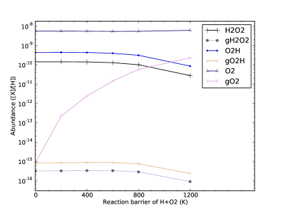
Figure 2: Dependence of the abundances of several species at the best-match time (6$\times$10⁵ yr) on the reaction barrier of reaction (3), with density fixed to 6$\times$10⁵ cm^-3 and temperature fixed to 21 K.

3.4 Effects of changing the diffusion energy barriers

The diffusion energy barrier of a species on the grain determines how fast it can migrate on the grain, so it basically determines the pace of the grain chemistry. Usually it is set to a fixed fraction (here we denote it by $\eta$) of the binding energy of each species. The latter determines how fast a species evaporates into the gas phase. However, this parameter might depend on the material and morphology of the dust grain, as well as the property of the adsorbate itself, so it is very uncertain. Values in the range of 0.3 – 0.77 have been adopted in the literature. We mainly used 0.77 for our modeling. Here we investigate how different values of $\eta$ would affect the abundances of several species of interest.

In Fig. 3 we plot the abundances of several species at the time of best-match (6$\times$10⁵ yr) as a function of the ratio between the diffusion barrier and binding energy ($\eta$). Changing this parameter has a large effect on the abundances of some species. For example, the abundance of CO₂ ice is reduced with a higher $\eta$. This is because at the time of concern it mainly forms through the reaction ${\rm OH+CO\rightarrow CO_{2}+H}$, which requires the migration of two relatively heavy species. With a low diffusion energy and a moderate temperature ($\sim$20 K), OH and CO can thermally hop quite fast, leading to a high abundance of CO₂, which is not observed. However, if a lower temperature ($\sim$10 K) is adopted, the problem becomes the opposite: the mobilities of OH and CO are so low that it is difficult for them to meet each other to form enough CO₂ ice, and certain intricate mechanism (e.g. three body reaction) has to be introduced to account for this (Garrod & Pauly 2011).

The abundance of H₂O ice increases as $\eta$ increases. At this stage it is mainly formed by hydrogenation of OH. As the mobility of atomic hydrogen on the grain is not greatly affected by the value of the diffusion energy barrier because it is allowed to migrate through quantum tunneling, the reaction rate of ${\rm H+OH\rightarrow H_{2}O}$ is not significantly affected by $\eta$; however, a larger $\eta$ leaves more OH available for water because a lower amount of it is consumed in forming CO₂. This is also the reason for a higher CO (and species dependent on it such as H₂CO and CH₃OH) ice abundance when $\eta$ is larger. The abundances of gas phase H₂O₂ and O₂H also increase for a larger $\eta$, albeit only mildly.

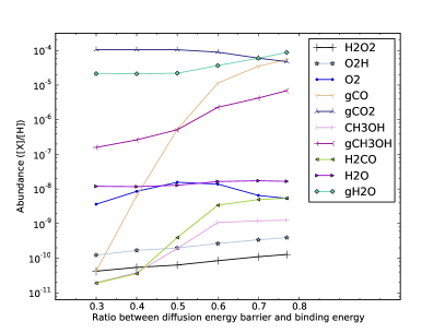
Figure 3: Dependence of the abundances of several species at the best-match time (6$\times$10⁵ yr) on the ratio between the diffusion and desorption energy, with density fixed to 6$\times$10⁵ cm^-3 and temperature fixed to 21 K.

3.5 Dependence on the temperature and density

The physical conditions (temperature and density) of $\rho$ Oph A are determined by non-LTE radiative transfer modeling (Bergman et al. 2011a), which is usually subject to uncertainties from many aspects, such as the excitation condition, source geometry, beam filling factor, etc. In this section we study how the uncertainties in the temperature and density of the system would affect the abundances of several species in our model. In Fig. 4 and Fig. 6 we plot the abundances of several species at the time of best-match (6$\times$10⁵ yr) as a function of temperature and density.

Apparently, temperature plays a much more drastic role than density. This is intuitively easy to understand because temperature enters the calculation of rates exponentially for the surface reactions. The general trend is that when the temperature is either too low or too high, the grain surface chemistry tends to be inactive or unimportant. In the former case the mobilities of species other than atomic hydrogen (which migrates through quantum tunneling in our present model) are low, while in the latter case the surface abundances of many species are low due to elevated evaporation rates.

As can be seen in Fig. 4, the abundance of CO ice starts to decrease at a temperature of around 20 K. This value can be estimated as the temperature at which the gas phase and grain surface abundance of CO are equal (see also Tielens & Hagen 1982), when only the adsorption and evaporation processes are taken into account (see also Hollenbach et al. 2009):

$$T_{\rm evap} =E_{\rm D}/\ln\left[\frac{\nu}{n_{\rm H}\;{R_{\rm G}}}\frac{1}{\pi r^{2}}\frac{1}{\sqrt{8kT_{\rm gas}/\pi m}}\right]$$ (6)

$$\simeq E_{\rm D}/\left\{60+\ln\left[\left(\frac{10^{5}\ {\rm cm}^{-3}}{n_{\rm H}}\right)\left(\frac{20\ {\rm K}}{T_{\rm gas}}\right)^{1/2}\left(\frac{m}{28\ {\rm au}}\right)^{1/2}\right]\right\},$$

where $E_{\rm D}$ is the evaporation energy barrier of a species on the grain surface, $\nu$ is the vibrational frequency of a species on the grain, ${R_{\rm G}}$ is the dust-to-gas number ratio, $r$ is the grain radius, while $m$ is the molecular mass of the species being considered. A typical value of 10¹² s^-1 for $\nu$, a dust grain radius of 0.1 $\mu$m, and a dust-to-gas ratio of 2.8$\times$10^-12 have been adopted in deriving the number 60. Since the logarithmic part in this equation is usually small for a typical gas density and temperature, the evaporation temperature can be approximated simply by $T_{\rm evap}\simeq E_{\rm D}/60$. For CO, a canonical value of $E_{\rm D}$ is 1210 K (Allen & Robinson 1977), which gives an evaporation temperature of 20 K, while for water, an $E_{\rm D}$ of 1860 K (Hasegawa & Herbst 1993) on bare graphite grains gives an evaporation temperature of $\sim$30 K. In Garrod & Herbst (2006) a much higher desorption energy of 5700 K for water is used (appropriate for water ice), which gives a evaporation temperature of $\sim$95 K, close to the observed evaporation temperature of water in envelope surrounding protostars (Maret et al. 2002). The evaporation temperature of CH₄ ice is close to that of CO ice. The evaporation time scale at the evaporation temperature can be estimated to be roughly $\nu^{-1}\exp(E_{\rm D}/T_{\rm evap})\simeq 10^{-12}e^{60}\ {\rm s}\simeq 3.6\times 10^{6}$ yr. For higher temperature the evaporation will be much faster.

The abundance of CO₂ ice initially increases with increasing temperature. This is because it mainly forms from the reaction ${\rm CO}+{\rm OH}\rightarrow{\rm CO}_{2}+{\rm H}$ with a barrier of 80 K, and an increase in temperature greatly enhances the mobility of the reacting species, as well as the probability of overcoming the reaction barrier. But when temperature increases more, the abundance of CO ice becomes so low that the CO₂ abundance also drops (the evaporation temperature of CO₂ is about 40 K thus evaporation is not responsible for the decline in CO₂ ice abundance seen in Fig. 4). A similar trend is seen in other species, such as H₂CO ice, CH₃OH ice, as well as gas phase H₂O₂, CH₃OH, H₂CO, and H₂O. On the other hand, for species efficiently produced in the gas phase, e.g. O₂, its abundance increases with temperature due to the faster evaporation at a higher temperature.

The abundances of gas phase H₂O₂, CH₃OH, CO, and O₂ have quite a sensitive dependence on temperature at around 21 – 24 K as seen from Fig. 4. For example, changing the temperature from 20 K to 22 K increases the abundance of H₂O₂ at a given time (6$\times$10⁵ yr) by about one order of magnitude. This rather small change of 2 K in temperature is normally smaller than the accuracy of the kinetic temperature as determined from observational data. The dependence of the evolution curves of H₂O₂ and CH₃OH on temperature can be seen more clearly in Fig. 5. Changing the temperature not only shifts the evolution curves horizontally, it also changes their shapes significantly. We can see that although for CH₃OH it is possible to match the observed abundance at multiple stages, for H₂O₂ the best match is only possible at 3$\times$10⁵ – 10⁶ yr (if we ignore the match in the very early stage).

Regarding the density dependence, Fig. 6 shows that the abundances of the gas phase species at 6$\times$10⁵ yr generally decrease with increasing density, because the accretion of molecules onto the dust grains is faster for a higher density. This does not necessarily mean that the abundances of the surface species always increase with density. For example, the abundances of CH₄ ice and CH₃OH ice decrease with higher density, while the abundance of H₂CO ice has the opposite trend. One important factor is the time when we look at the system. In Fig. 7 we plot the abundances of H₂CO ice and CH₃OH ice as a function of time for different densities, while the temperature is fixed at 21 K. It can be seen that at a given time, the abundances of H₂CO ice or CH₃OH ice can either increase or decrease when the density is increased. We note that the evolution curves of these species have a quasi-oscillatory feature. For the same species, the evolution curves have a similar shape for different densities, except that with a lower density the evolution is slower and thus the curves are shifted rightward.

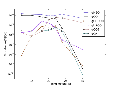
Figure 4: Dependence of the abundances of several species at the time of best-match (6$\times$10⁵ yr) on temperature, with density fixed to 6$\times$10⁵ cm^-3. Left panel: gas phase species; right panel: surface species.

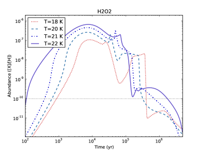
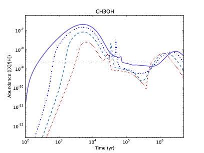
Figure 5: The abundances of gas phase H₂O₂ and CH₃OH as a function of time for different temperatures. The density is fixed to 6$\times$10⁵ cm^-3. The horizontal dotted lines mark the observed abundances of the corresponding species.

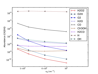
Figure 6: Dependence of the abundances of several species at the time of best-match (6$\times$10⁵ yr) on n_H, with temperature fixed to 21 K. Left panel: gas phase species; right panel: surface species.

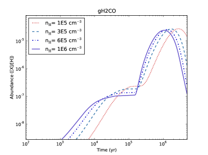
Figure 7: The abundances of H₂CO and CH₃OH ice as a function of time for different densities. The temperature is fixed to 21 K.

3.6 Discussions and limits of the model

It can be seen from Fig. 1, Fig. 6, and Fig. 5 that H₂O₂ can be produced with a rather high abundance at certain evolution stages or with certain physical parameters, which is frequently higher than the current observed value (Bergman et al. 2011b), especially in the early to intermediate time ($\sim$10³ – 10⁵ yr). One natural question to ask is why H₂O₂ has not been commonly detected in the interstellar medium. One possibility is that its spectral lines have been overlooked in the past. Another simple explanation would be that it is over-produced in our model, because in the past the chemistry of H₂O₂ (as well as O₂H and O₃, etc.) may not have been studied in detail in the astro-chemistry context (especially the destruction reactions in the gas phase), so that its destruction routes might be incomplete. For example, there is no reaction in which H₂O₂ is destroyed by reacting with H${}_{3}^{+}$ in the current mainstream gas phase chemical networks. As a rough estimate, if we take the rate of destruction by such a reaction to be the same as the rate of the reaction ${\rm H_{3}^{+}+H_{2}O\rightarrow H_{3}O^{+}+H_{2}}$, then the abundance of gas phase H₂O₂ can be reduced by about one order of magnitude. Further theoretical/experimental studies of the H₂O₂ chemistry would thus be very helpful, given the fact that it has been detected recently and its potential important role in the grain chemistry of water. A third possibility is that the rarity of H₂O₂ might be an age effect. From Fig. 5 we notice that the abundance of H₂O₂ is very high only in a relatively early stage (before $\sim$5$\times$10⁵ yr). If for certain reason most of the cloud cores being observationally studied are older than this (due to some selection effects), then the H₂O₂ abundance in these objects would be too low to detect. Basically, at least three physical parameters, namely age, density, and temperature, are relevant. A probability distribution of these three parameters of the cloud cores would help to give the detection probability of H₂O₂ (and any other molecules). In this sense, $\rho$ Oph A may be considered special in the sense that it has a relatively high density ($\sim$10⁶ cm^-3) and temperature (20 – 30 K), while most dark clouds with a high density ($\gtrsim$10⁴ cm^-3) tend to be very cold ($\lesssim$15 K) (Bergin & Tafalla 2007). An inhomogeneous physical condition would make the situation more complex, which may require a self-consistent dynamical-chemical model. However, a thorough study on these possibilities has to be left for future work.

On the other hand, for CH₃OH, although it has been studied quite extensively in the past, we notice that the gas phase reactions associated with it contain some important (although not decisive) differences between the OSU09 network and the UMIST RATE06 network. For example, the reaction between CH and CH₃OH to form CH₃ and H₂CO has a rate 2.49$\times$10^-10$(T/300)^{-1.93}$ in the UMIST RATE06 network, but it does not exist in the OSU09 network. One possible problem is that the temperature of cold interstellar medium (at most several tens of Kelvins) is out of the indicated valid range for many reactions in RATE06, and it is not clear how to extrapolate these reaction rates correctly, although we have closely followed the instructions in Woodall et al. (2007). In our modeling we have been using the RATE06 network.

The energy barriers for the hydrogenation of CO and H₂CO on the grain are both taken to be 2500 K. Woon (2002) calculated the barrier heights of these two reactions, giving a value of $\sim$2740 K and 3100 K, respectively, in the case three water molecules are present, with zero point energy corrections added. If these values were adopted, then the observed abundances of H₂CO and CH₃OH can only be reproduced within one order of magnitude at best. However, Goumans (2011) gives a lower barrier height ($\sim$2200 K) for the hydrogenation of H₂CO, which would give a better agreement with the observational results than if Woon (2002) were used in our model.

The chemical desorption is very important for the abundances of the gas phase H₂O₂ and CH₃OH. However, the efficiency of this mechanism (the “$a$” parameter in Garrod et al. (2007)) is uncertain. Garrod & Pauly (2011) adopted a low value of 0.01 for it, to avoid over-production of some gas phase species (Garrod et al. 2007). We use a value of $0.1$ in our study, and the abundances of H₂CO and CH₃OH are not over-produced, except possibly in the early stages of the evolution. We note that the temperature and density of major concern in our study is around 20 K and 6$\times$10⁵ cm^-3, while in Garrod et al. (2007) the temperature and density are set to 10 K and 2$\times$10⁴ cm^-3, respectively. As a test we run our model with the latter physical condition, and in this case CH₃OH and H₂CO are indeed over-produced by about one order of magnitude. Thus it seems that the efficiency of chemical desorption depends on the temperature of the dust grain, in the sense that at higher temperature the probability that the product of a surface exothermic reaction gets ejected to the gas phase is higher. However, a detailed study of this possibility is out of the scope of the present paper.

Regarding the formation of water ice, Bergin et al. (1998) proposed an interesting mechanism in which water is first formed in the high temperature shocked gas, and then gets adsorbed onto the dust grains in the post-shock phase. This mechanism may act as an alternative or supplement to the grain chemistry route. It is not our aim here to discuss to what extent this mechanism contributes to the water ice budget. However, we remark that even with a temperature 1000 – 2000 K, the amount of H₂O₂ produced in a pure gas phase chemistry (using the UMIST RATE06 network) is still much lower than the detected level.

4 Conclusions

With a gas-grain chemical model which properly takes into account the desorption of grain surface species by the heat released by chemical reactions, we reproduce the observed abundances of H₂O₂ in $\rho$ Oph A at a time of $\sim$6$\times$10⁵ yr. The solid phase H₂O₂ abundance is very low in this stage. However, a H₂O₂ to H₂O ratio of a few percent might be obtained in the solid phase if the layered structure of grain mantle is taken into account.

The abundances of other species such as H₂CO, CH₃OH, and O₂ detected in the same object can also be reasonably reproduced at a time of $\sim$6$\times$10⁵ yr. Such a time scale is consistent with the evolution time scale estimated through dynamical considerations.

O₂H is a precursor of H₂O₂ on the dust grain, and we predict that it has a gas-phase abundance with the same order-of-magnitude of H₂O₂ and should thus be detectable. Observational searches for it are under way.

For physical conditions relevant to $\rho$ Oph A, water is mainly in solid form, being the dominant grain mantle material. Its gas phase abundance is only of the order of 10^-8 according to our model.

We note that the abundance of gas-phase H₂O₂ in our model results can be much higher than the current observed level for a range of physical conditions. This may suggest that its gas phase destructing channels are incomplete. Due to the potential important role played by H₂O₂ in the formation of water, its reaction network needs to be studied more thoroughly in the future.

Other uncertainties in our modeling include the ratio between the diffusion energy barrier to the binding energy of a species on the grain surface, the activation energy barriers of certain key reactions, as well as the efficiency of the chemical desorption mechanism. In the present work we mainly make use of their canonical values, or values which give good match to the observational results, and we also vary them to see the effects on the resulting abundances, which are significant in many cases.

Appendix A An explanation of the spike-like features in the evolution curves

In Fig. 1 we note that at a time of $\sim$5$\times$10⁴ yr a spike-like feature appears in the evolution curves of some species (e.g. gas phase H₂O₂ and CH₃OH), while the abundances of some other species (e.g. H₂O₂ and O₂ on the grain) change very rapidly at the same time. While these features may appear to be caused by faults in the program for solving the set of differential equations, however, after solving the same problem with the Monte Carlo method which is immune to such numerical instabilities, we find that these features are still present, indicating that they are genuine. How could a smooth ordinary differential equation system generate such an almost-singular feature? In Fig. 8 we make a zoom-in of Fig. 1 (with several species added and several species removed). It can be seen that although the time scale of the spike-like feature is relatively short, the evolution is always smooth (except the discreteness caused by the finite sampling of the curve). Then what determines the appearance of such a feature?

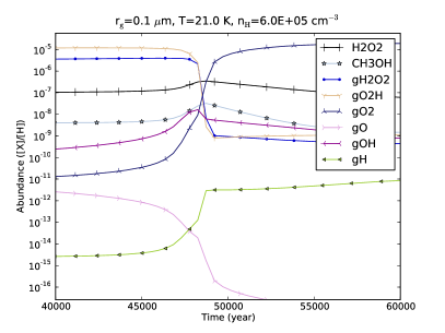
Figure 8: A zoom-in plot of Fig. 1 (with several species removed and several added), focusing on the spike-like feature (though nothing looks like a spike anymore). The abundance of gH has been multiplied by a factor of 10¹² (to make the plot look more compact).

As atomic hydrogen is central to the surface chemistry, we first look at the most important reactions governing its abundance on the grain. The main reactions consuming atomic hydrogen on the grains are (in the following a species name preceded by a “g” means a species on the grain, otherwise it is in the gas phase)

$${\rm gH+gO_{2}H}\xrightarrow{k_{1}}\left\{\begin{aligned} &{\rm gOH+gOH,}\\ &{\rm gH_{2}O_{2},}\\ &{\rm OH+OH,}\\ &{\rm H_{2}O_{2},}\end{aligned}\right.$$ (7)

$${\rm gH+gH_{2}O_{2}}\xrightarrow{k_{2}}\left\{\begin{aligned} &{\rm gH_{2}O+gOH},\\ &{\rm H_{2}O+OH},\end{aligned}\right.$$ (8)

while others such as the reactions with gO₃ and gCH₂OH are relatively unimportant in the early times. It is mainly produced by

$${\rm H\xrightarrow{k_{3}}gH,}$$ (9)

$${\rm gOH+gCO\xrightarrow{k_{4}}gCO_{2}+gH,}$$ (10)

$${\rm gH_{2}O\xrightarrow{k_{5}}gOH+gH.}$$ (11)

As the abundance of atomic H in the gas phase and the abundance of gCO and gH₂O change relatively smoothly, they can be viewed as constant in a short time scale. The main reactions for the consumption and production of gOH are

$${\rm gO+gOH}\xrightarrow{k_{6}}\left\{\begin{aligned} &{\rm gO_{2}H,}\\ &{\rm O_{2}H,}\\ \end{aligned}\right.$$ (12)

$${\rm gCO+gOH}\xrightarrow{k_{7}}\left\{\begin{aligned} &{\rm gCO_{2}+gH,}\\ &{\rm CO_{2}+H,}\\ \end{aligned}\right.$$ (13)

$${\rm gH+gO_{2}H}\xrightarrow{k_{8}}{\rm gOH+gOH,}$$ (14)

$${\rm gH+gH_{2}O_{2}}\xrightarrow{k_{9}}{\rm gH_{2}O+gOH},$$ (15)

$${\rm gH_{2}O}\xrightarrow{k_{10}}{\rm gH+gOH}.$$ (16)

From the above reaction list we may write the evolution equation of gH and gOH as

$$\partial_{t}{\rm gH}= -k_{1}{\rm gHgO_{2}H}-k_{2}{\rm gHgH_{2}O_{2}}$$

$$+k_{3}{\rm H}+k_{4}{\rm gOHgCO}+k_{5}{\rm gH_{2}O},$$ (17)

$$\partial_{t}{\rm gOH}= -k_{6}{\rm gOgOH}-k_{7}{\rm gCOgOH}$$

$$+2k_{8}{\rm gHgO_{2}H}+k_{9}{\rm gHgH_{2}O_{2}}+k_{10}{\rm gH_{2}O},$$ (18)

or in a more succinct form

$$\partial_{t}{\rm gH}= \kappa_{1}{\rm gH}+\kappa_{2}{\rm gOH}+b_{1},$$

$$\partial_{t}{\rm gOH}= \kappa_{3}{\rm gH}+\kappa_{4}{\rm gOH}+b_{2},$$ (19)

where

$$\kappa_{1}= -k_{1}{\rm gO_{2}H}-k_{2}{\rm gH_{2}O_{2}},$$

$$\kappa_{2}= k_{4}{\rm gCO},$$

$$\kappa_{3}= 2k_{8}{\rm gO_{2}H}+k_{9}{\rm gH_{2}O_{2}},$$

$$\kappa_{4}= -k_{6}{\rm gO}-k_{7}{\rm gCO},$$

$$b_{1}= k_{3}{\rm H}+k_{5}{\rm gH_{2}O},$$

$$b_{2}= k_{10}{\rm gH_{2}O}.$$

If we view $\kappa_{1}$ – $\kappa_{4}$ as well as $b_{1}$ and $b_{2}$ as constants (of course they are not), then equation (19) can be solved exactly; the solution contains an exponential part and a constant part. The amplitude of the exponential part will be inversely proportional to the determinant of the coefficient matrix

$${\rm det}(\kappa)=\left(\begin{array}[]{cc}\kappa_{1}&\kappa_{2}\\ \kappa_{3}&\kappa_{4}\end{array}\right).$$

As $\kappa_{1}$ – $\kappa_{4}$ are not really constant in our problem, we expect that when they become such that det($\kappa$) is close to zero, a spike-like or jump-like behavior would appear. Namely, we require

$$\frac{\kappa_{1}\kappa_{4}}{\kappa_{2}\kappa_{3}}= \frac{(k_{1}{\rm gO_{2}H}+k_{2}{\rm gH_{2}O_{2}})(k_{6}{\rm gO}+k_{7}{\rm gCO})}{(k_{4}{\rm gCO})(2k_{8}{\rm gO_{2}H}+k_{9}{\rm gH_{2}O_{2}})}$$

$$\simeq \frac{{\rm gO_{2}H/gH_{2}O_{2}+1}}{1.2{\rm gO_{2}H/gH_{2}O_{2}}+1}\times\left(2.5\times 10^{8}{\rm gO/gCO+1}\right)$$

$$\simeq 1.$$ (20)

In the second line of the above equation the actual value of the parameters have been inserted. These parameters depend on the physical conditions.

To satisfy this condition (at least approximately), gO/gCO should be very small. In Fig. 9 the ratio $(\kappa_{1}\kappa_{4})/(\kappa_{2}\kappa_{3})$ and the value of 2.5$\times$10⁸gO/gCO are plotted as a function of time. The abundances of O, gO, gO₂, gH, and gOH are also plotted for reference (not to scale). It can be seen that the $(\kappa_{1}\kappa_{4})/(\kappa_{2}\kappa_{3})$ ratio does decrease and approach a value of unity before the time of the spike/jump feature, and the gO/gCO ratio does drop to a very low value monotonically.

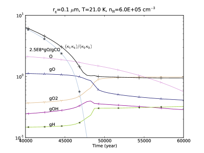
Figure 9: The ratio $(\kappa_{1}\kappa_{4})/(\kappa_{2}\kappa_{3})$ and the value of 2.5$\times$10⁸$\times$gO/gCO as a function of time. They are to scale. The abundances of several other species are plotted only for reference (not to scale).

The above mathematical argument can also be understood intuitively. When the gO abundance is so low that reaction (12) can be neglected, gOH is only destroyed by reaction (13). Each time a gOH radical is consumed, one gH is created (if we neglect the desorption process), and this gH will quickly react with gH₂O₂ or gO₂H to create one or two gOHs. So there will be a net gain in the gOH abundance, leading to its fast growth, and the gH abundance will increase accordingly. Thus we see that reaction (14) is crucial in that it produced two gOH radicals by consuming only one gH.

Therefore for such a spike-like feature to occur, the abundance of gO must decrease to a low value such that the reaction between gOH and gO becomes unimportant in consuming gOH. Namely, we require ${\rm[gO]\lesssim[gCO]\ k_{7}/k_{6}}\simeq 5\times 10^{-13}$. The abundances of atomic oxygen in the gas phase and on the grain surface are related by ${\rm O/gO\simeq k_{\rm evap}(gO)/k_{\rm ad}(O)\simeq 3\times 10^{6}}$, so equivalently we require ${\rm[O]<1.5\times 10^{-6}}$ (i.e. about a factor of 200 less than the initial O abundance) at the time of the spike-like feature. Atomic oxygen is mainly consumed on the grain surface by reacting with another gO to form gO₂ (for $t\lesssim 10^{3}$ yr) or by reacting with gOH to form gO₂H. Only the latter is relevant here. As the abundance of gOH does not change much before the spike-like feature, the time scale for the consumption of atomic oxygen can be estimated to be ${\ln 200\times({\rm O/gO})/(k_{6}{\rm gOH})}\simeq 10^{5}$ yr, which is of the same order of magnitude of the time of occurrence of the spike-like feature.

The time scale for the endurance of the spike-like feature itself can be estimated to be the time scale for the exhaustion of gO₂H or gH₂O₂ (so that equations (17) and (18) do not hold anymore) by reacting with gH, which is

$$1/(k_{1}{\rm gH})\simeq 10^{3}\ {\rm yr},$$

where the gH population (the average number of atomic H on a single grain) is taken to be a median value (10^-14) during the rapidly-varying period. The fact that equation (20) seems to hold after this period (see Fig. 9) does not mean that gH will keep increasing rapidly, simply because the premise of our argument, namely equations (17) and (18) are not a good description of the evolution of gH and gOH anymore.

As the abundance of H on the grain increases, almost all the O₃ on the grain are converted into O₂ and OH. O₂ molecules on the grain are then consumed by the slower reaction ${\rm gH+gO_{2}\rightarrow gO_{2}H}$, with a time scale $\sim$10⁵ yr. This explains the prominent peak in the evolution curve of gO₂ (see Fig. 1).

Would the spike-like feature have any practical significance (especially observationally)? Ideally, such a short-time feature may be used to contrain the age of a dense cloud, by discrimiating the abundances of certain species between their early-time values (before the spike-like feature) and late-time values (after the spike-like feature). However, due to its dependence on the reaction network being used, which usually contains a lot of uncertainties and is subject to change when new experiments are carried out, the question whether this feature is really relevant for the study of interstellar medium can only be answered by future investigations.

Appendix B The surface reaction network used in this work

HHL92: Hasegawa et al. (1992); ICet10: Ioppolo et al. (2010); CIRL10: Cuppen et al. (2010); ICet08: Ioppolo et al. (2008); G11: Goumans (2011); FCet09: Fuchs et al. (2009) GWH08: Garrod et al. (2008); AR77: Allen & Robinson (1977); TH82: Tielens & Hagen (1982); GMet08: Goumans et al. (2008); ABet04: Atkinson et al. (2004); RH00: Ruffle & Herbst (2000); RH01: Ruffle & Herbst (2001b);

Table 1: The surface network used in this work. The photo-dissociation reactions induced by cosmic rays and the chemical desorption reactions are not included here.

Num	Reaction	Branching ratio	Energy barrier (K)	Reference
1	H + H $\rightarrow$ H2	1.0	0.0	HHL92
2	H + O $\rightarrow$ OH	1.0	0.0	ICet10
3	H + O2 $\rightarrow$ O2H	1.0	600.0	Estimated
4	H + O3 $\rightarrow$ O2 + OH	1.0	200.0	Estimated
5	H + OH $\rightarrow$ H2O	1.0	0.0	ICet10
6	H + O2H $\rightarrow$ H2O2	0.38	0.0	CIRL10
7	H + O2H $\rightarrow$ OH + OH	0.62	0.0	CIRL10
8	H + H2O2 $\rightarrow$ H2O + OH	1.0	0.0	ICet08
9	H + CO $\rightarrow$ HCO	0.5	2500.0	GWH08
10	H + HCO $\rightarrow$ H2CO	1.0	0.0	FCet09
11	H + H2CO $\rightarrow$ CH3O	0.5	2500.0	RH00
12	H + H2CO $\rightarrow$ HCO + H2	0.5	3000.0	G11
13	H + CH3O $\rightarrow$ CH3OH	1.0	0.0	FCet09
14	H + CH2OH $\rightarrow$ CH3OH	1.0	0.0	GWH08
15	H + HCOO $\rightarrow$ HCOOH	1.0	0.0	AR77
16	H + C $\rightarrow$ CH	1.0	0.0	AR77
17	H + CH $\rightarrow$ CH2	1.0	0.0	AR77
18	H + CH2 $\rightarrow$ CH3	1.0	0.0	AR77
19	H + CH3 $\rightarrow$ CH4	1.0	0.0	AR77
20	H + N $\rightarrow$ NH	1.0	0.0	AR77
21	H + NH $\rightarrow$ NH2	1.0	0.0	AR77
22	H + NH2 $\rightarrow$ NH3	1.0	0.0	AR77
23	H + S $\rightarrow$ HS	1.0	0.0	HHL92
24	H + HS $\rightarrow$ H2S	1.0	0.0	HHL92
25	H + H2S $\rightarrow$ HS + H2	1.0	860.0	TH82
26	H + CS $\rightarrow$ HCS	1.0	0.0	HHL92
27	C + S $\rightarrow$ CS	1.0	0.0	HHL92
28	O + S $\rightarrow$ SO	1.0	0.0	HHL92
29	O + SO $\rightarrow$ SO2	1.0	0.0	HHL92
30	O + CS $\rightarrow$ OCS	1.0	0.0	HHL92
31	H + CN $\rightarrow$ HCN	1.0	0.0	AR77
32	H + NO $\rightarrow$ HNO	1.0	0.0	AR77
33	H + NO2 $\rightarrow$ HNO2	1.0	0.0	AR77
34	H + NO3 $\rightarrow$ HNO3	1.0	0.0	AR77
35	H + N2H $\rightarrow$ N2H2	1.0	0.0	AR77
36	H + N2H2 $\rightarrow$ N2H + H2	1.0	650.0	HHL92
37	H + NHCO $\rightarrow$ NH2CO	1.0	0.0	AR77
38	H + NH2CO $\rightarrow$ NH2CHO	1.0	0.0	AR77
39	N + HCO $\rightarrow$ NHCO	1.0	0.0	AR77
40	CH + CH $\rightarrow$ C2H2	1.0	0.0	HHL92
41	O + O $\rightarrow$ O2	1.0	0.0	AR77
42	O + O2 $\rightarrow$ O3	1.0	0.0	ABet04
43	O + CO $\rightarrow$ CO2	1.0	1580.0	GMet08
44	O + HCO $\rightarrow$ HCOO	0.5	0.0	GMet08
45	O + HCO $\rightarrow$ CO2 + H	0.5	0.0	GMet08
46	O + N $\rightarrow$ NO	1.0	0.0	AR77
47	O + NO $\rightarrow$ NO2	1.0	0.0	AR77
48	O + NO2 $\rightarrow$ NO3	1.0	0.0	AR77
49	O + CN $\rightarrow$ OCN	1.0	0.0	AR77
50	C + N $\rightarrow$ CN	1.0	0.0	AR77
51	N + N $\rightarrow$ N2	1.0	0.0	AR77
52	N + NH $\rightarrow$ N2H	1.0	0.0	AR77
53	H2 + OH $\rightarrow$ H2O + H	1.0	2100.0	ABet04
54	OH + CO $\rightarrow$ CO2 + H	1.0	80.0	RH01
55	H + C2 $\rightarrow$ C2H	1.0	0.0	HHL92
56	H + N2 $\rightarrow$ N2H	1.0	1200.0	HHL92
57	H + C2H $\rightarrow$ C2H2	1.0	0.0	HHL92
58	H + HOC $\rightarrow$ CHOH	1.0	0.0	HHL92
59	C + OH $\rightarrow$ HOC	0.5	0.0	HHL92
60	C + OH $\rightarrow$ CO + H	0.5	0.0	HHL92
61	CH + OH $\rightarrow$ CHOH	1.0	0.0	HHL92
62	H + CHOH $\rightarrow$ CH2OH	1.0	0.0	HHL92
63	OH + OH $\rightarrow$ H2O2	1.0	0.0	HHL92
64	OH + CH2 $\rightarrow$ CH2OH	1.0	0.0	HHL92
65	C + C $\rightarrow$ C2	1.0	0.0	HHL92
66	C + O2 $\rightarrow$ CO + O	1.0	0.0	HHL92
67	O + CH $\rightarrow$ HCO	1.0	0.0	HHL92
68	O + OH $\rightarrow$ O2H	1.0	0.0	HHL92
69	O + CH2 $\rightarrow$ H2CO	1.0	0.0	HHL92
70	O + CH3 $\rightarrow$ CH2OH	1.0	0.0	HHL92
71	C + O $\rightarrow$ CO	1.0	0.0	HHL92
72	C + CH $\rightarrow$ C2H	1.0	0.0	HHL92
73	C + NH $\rightarrow$ HNC	1.0	0.0	HHL92
74	C + CH2 $\rightarrow$ C2H2	1.0	0.0	HHL92
75	C + NH2 $\rightarrow$ HNC + H	1.0	0.0	HHL92
76	N + CH $\rightarrow$ HCN	1.0	0.0	HHL92
77	N + NH2 $\rightarrow$ N2H2	1.0	0.0	HHL92
78	O + NH $\rightarrow$ HNO	1.0	0.0	HHL92

Table 1: continued.

Appendix C The enthalpies of the surface species

BM02: Binnewies & Milke (1999); NIST Webbook: http://webbook.nist.gov/chemistry/; NCet10: Nagy et al. (2010); K98: Kaiser et al. (1998); VS91: Vandooren et al. (1991); Url1: http://chem.engr.utc.edu/webres/331f/teams-98/chp/Boiler%20DC/tsld007.htm

Table 2: Enthalpies of the surface species considered in this work. They are used to calculate the exoergicities of the surface reactions.

Num	Species	Enthalpy (kJ/mol)	Reference
1	C	716.7	NIST Webbook
2	CH	594.1	BM02, p238
3	CH2	386.4	BM02, p240
4	CH3	145.7	BM02, p241
5	CH3O	17.0	NIST Webbook
6	CH2OH	-9.0	NIST Webbook
7	CH3OH	-201.2	BM02, p241
8	CH4	-74.9	BM02, p241
9	CN	435.1	BM02, p247
10	CO	-110.5	BM02, p251
11	CO2	-393.5	BM02, p251
12	CS	280.3	BM02, p253
13	H	218.0	BM02, p558
14	H2	0.0	BM02, p568
15	H2CO	-115.9	BM02, p240
16	H2O	-241.8	BM02, p571
17	H2O2	-135.8	BM02, p572
18	H2S	-20.5	BM02, p574
19	HCN	135.1	BM02, p239
20	HNC	135.1	Estimated
21	HCO	43.5	BM02, p239
22	HCOO	-386.8	Url1
23	HCOOH	-378.6	BM02, p240
24	HCS	296.2	K98
25	HNO	99.6	BM02, p563
26	HNO2	-78.8	BM02, p563
27	HNO3	-134.3	BM02, p563
28	HS	139.3	BM02, p567
29	N	472.7	BM02, p693
30	N2	0.0	BM02, p699
31	N2H	245.2	VS91
32	N2H2	213.0	BM02, p570
33	NH	376.6	BM02, p563
34	NH2	190.4	BM02, p570
35	NH2CHO	-186.0	NIST Webbook
36	NH2CO	-13.1	NCet10
37	NH3	-45.9	BM02, p577
38	NHCO	-101.7	BM02, p239
39	NO	90.3	BM02, p695
40	NO2	33.1	BM02, p695
41	NO3	71.1	BM02, p695
42	O	249.2	BM02, p733
43	O2	0.0	BM02, p741
44	O2H	2.1	BM02, p567
45	O3	142.7	BM02, p752
46	OCN	159.4	BM02, p248
47	OCS	-138.4	BM02, p251
48	OH	39.0	BM02, p566
49	S	277.0	BM02, p811
50	SO	5.0	BM02, p736
51	SO2	-296.8	BM02, p743
52	C2	837.74	NIST Webbook
53	C2H	476.98	NIST Webbook
54	C2H2	226.73	NIST Webbook

Table 2: continued.