Abstract

We estimate possible systematic error that can arise in the simplified simulation of the $W_{R}$ production and its subsequent decay into heavy neutrino at LHC (left-right symmetric model). The general-purpose event generators simulate this process as a $W_{R}$ production followed by two decays, loosing full information about the polarization of the intermediate particles. We calculate the cross section using the full matrix elements with propagators, perform the simulation and compare the results with the simplified simulation.

1 Introduction

It is known that in the Standard Model there are left-handed W-bosons that interact with left-handed fermions. The Left-right symmetric model (for more details see [1]) states that there are also right-handed W bosons interacting with right handed-fermions. In the minimal Left-right symmetric model they have the same coupling constants to the fermions but are much heavyer, otherwise they would be already discovered. In other words, in the SM the terms responsible for the interaction between fermions and weak bosons are

$$i\bar{Q_{L}}\gamma^{\mu}\left(\partial_{\mu}-\frac{ig}{2}\vec{\tau}\vec{(}W_{L})_{\mu}-\frac{ig^{\prime}}{6}B_{\mu}\right)Q_{L}+$$

$$i\bar{\psi_{L}}\gamma^{\mu}\left(\partial_{\mu}-\frac{ig}{2}\vec{\tau}\vec{(}W_{L})_{\mu}+\frac{ig^{\prime}}{2}B_{\mu}\right)\psi_{L}.$$ (1)

Here Q are quark doublets and $\psi$ are lepton doublets. The Left-right symmetric model contains also the following terms:

$$i\bar{Q_{R}}\gamma^{\mu}\left(\partial_{\mu}-\frac{ig}{2}\vec{\tau}\vec{(}W_{R})_{\mu}-\frac{ig^{\prime}}{6}B_{\mu}\right)Q_{R}+$$

$$i\bar{\psi_{R}}\gamma^{\mu}\left(\partial_{\mu}-\frac{ig}{2}\vec{\tau}\vec{(}W_{R})_{\mu}+\frac{ig^{\prime}}{2}B_{\mu}\right)\psi_{R}.$$ (2)

The lepton doublets here contain ordinary charged leptons and heavy right-handed neutrinos. We assume that they can be Dirac or Majorana neutrinos.

The searches for these new particles are being performed now at LHC [2]. The purpose of this work is to estimate possible systematic errors arising from some approximations usually used in the simulation of the signal by general purpose event generators.

We consider the following process. $d$-quark and $u$-antiquark interact with each other producing the $W^{-}_{R}$ -boson. It decays into the lepton $L1$ and heavy antineutrino $N$ that decays into another lepton $L2$, $u$-antiquark and $d$-quark via the virtual $W^{-}_{R}$-boson. This process is represented in Figure 1.

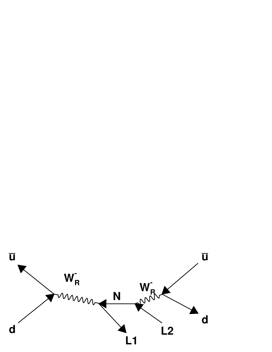
Figure 1: Diagram with Dirac neutrino

This process takes place regardless of the type of the neutrino: it can be either Dirac-like or Majorana-like. However if the neutrino is Majorana-like, another process is possible with the same initial particles: $d\bar{u}\to L_{1}L_{2}u\bar{d}$ (it is drawn in Figure 2).

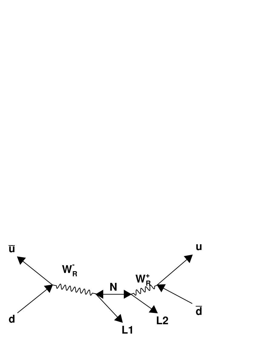
Figure 2: Diagram possible with Majorana heavy neutrino (leptons have same sign)

The cross-section of these reactions can be calculated explicitly. However, the 4 - particle final state is too complicated for the general purpose event generators (for example pythia6 [3]) usually used in the HEP analyses. In such generators this process is considered in the following approximate way: quark-antiquark pair produces real $W^{-}$-boson, then it decays into real lepton $L2$ and antineutrino and the antineutrino decays into antilepton $L2$ and quark-antiquark pair (if the neutrino is Majorana-like it can decay either to lepton or to antilepton). In this case the information about the polarization of intermediate particles is lost. We consider both approaches and compare the results they give. Let us note that we neglect other possible reactions with the same initial and final state particles.

2 Cross section with the full matrix element

Let the particles in our process have the following momenta:

• -momentum of the initial $d$-quark

• -momentum of the initial $u$-antiquark

• -momentum of the lepton $L1$

• -momentum of the lepton $L2$

• -momentum of the final $d$-quark

• -momentum of the final $u$-antiquark

The amplitude of the reaction represented in Figure 1 is written in the following way (here we use the common notations that can be found for example in [4], [5]):

$$\bar{v}(p_{2})\frac{ig}{\sqrt{2}}\gamma^{\mu}\frac{(1+\gamma^{5})}{2}u(p_{1})\frac{-i}{(p_{1}+p_{2})^{2}-M_{W}^{2}}\left(g_{\mu\nu}\frac{(p_{1}+p_{2})_{\mu}(p_{1}+p_{2})_{\nu}}{M_{W}^{2}}\right)$$

$$\bar{u}(k_{1})\frac{ig}{\sqrt{2}}\gamma^{\nu}\frac{(1+\gamma^{5})}{2}\frac{i(\hat{p}_{1}+\hat{p}_{2}-\hat{k}_{1})+m_{\nu}}{(p_{1}+p_{2}-k_{1})^{2}-m_{\nu}^{2}}\frac{ig}{\sqrt{2}}\gamma^{\lambda}\frac{(1+\gamma^{5})}{2}v(k_{2})$$

$$\frac{-i}{(q_{1}+q_{2})^{2}-M_{W}^{2}}\left(g_{\lambda\rho}\frac{(q_{1}+q_{2})_{\lambda}(q_{1}+q_{2})_{\rho}}{M_{W}^{2}}\right)\frac{ig}{\sqrt{2}}\bar{u}(q_{1})\gamma^{\rho}\frac{(1+\gamma^{5})}{2}v(q_{2})$$ (3)

Here we do not take into account any possible mixings among the particles. Further we also neglect the masses of all particles except $W^{-}$boson and the neutrino. Using the standard rules (see [4]) one can show that

$$|M|^{2}=\frac{4g^{8}(k_{1}p_{2})(q_{2}k_{2})((k_{1}p_{2})(p_{1}q_{1})+(p_{1}(k_{1}-p_{2}))(q_{1}(k_{1}-p_{2})))}{((p_{1}+p_{2})^{2}-M_{W}^{2})^{2}((q_{1}+q_{2})^{2}-M_{W}^{2})((p_{1}+p_{2}-k_{1})^{2}-m_{\nu}^{2})}$$ (4)

We used the mathematica package feyncalc to obtain this expression.

Then this formula is substituted into the general expression for cross-section of massless particles [6]

$$d\sigma=\frac{1}{(2\pi)^{8}}\delta^{(4)}(k_{1}+k_{2}+q_{1}+q_{2}-p_{1}-p_{2})|M|^{2}\frac{1}{4(p_{1}p_{2})}\frac{d^{3}\vec{k}_{1}d^{3}\vec{k}_{2}d^{3}\vec{q}_{1}d^{3}\vec{q}_{2}}{16k_{1}^{0}k_{2}^{0}q_{1}^{0}q_{2}^{0}}$$ (5)

The delta-function of spatial momenta is taken off by integration over $q_{2}$. To take off the delta-function over energy we rewrite

$$d^{3}q_{1}=|\vec{q}_{1}|^{2}d|\vec{q}_{1}|\sin\theta d\theta d\varphi$$

where $\theta$ and $\varphi$ is polar and axial angle relative to the vector $\vec{k}_{1}+\vec{k}_{2}-\vec{p}_{1}-\vec{p}_{2}$. We also rewrite the argument of the delta-function as

$$|\vec{q}_{1}|+\sqrt{|\vec{q}_{1}|^{2}+|\vec{k}_{1}+\vec{k}_{2}-\vec{p}_{1}-\vec{p}_{2}|^{2}+2|\vec{q}_{1}||\vec{k}_{1}+\vec{k}_{2}-\vec{p}_{1}-\vec{p}_{2}|\cos\theta}+$$

$$|\vec{k}_{1}|+|\vec{k}_{2}|-|\vec{p}_{1}|-|\vec{p}_{2}|$$

After integration over $|\vec{q}_{1}|$ we obtain

$$d\sigma=\frac{4g^{8}(k_{1}p_{2})(q_{2}k_{2})((k_{1}p_{2})(p_{1}q_{1})+(p_{1}(k_{1}-p_{2}))(q_{1}(k_{1}-p_{2})))}{(2\pi)^{8}(((p_{1}+p_{2})^{2}-M_{W}^{2})^{2}+M_{W}^{2}\Gamma_{W}^{2})(((q_{1}+q_{2})^{2}-M_{W}^{2})^{2}+M_{W}^{2}\Gamma_{W}^{2})}$$

$$\frac{|\vec{q}_{1}|d^{3}\vec{k}_{1}d^{3}\vec{k}_{2}d\theta\sin\theta d\varphi}{16(p_{1}p_{2})(((p_{1}+p_{2}-k_{1})^{2}-m_{\nu}^{2})^{2}+m_{\nu}^{2}\Gamma_{\nu}^{2})|\vec{k}_{1}||\vec{k}_{2}|(|\vec{q}_{1}|+|\vec{q}_{2}|+|\vec{q}_{1}+\vec{q}_{2}|\cos\theta)}$$ (6)

Here we also introduced the $\Gamma_{W}$, $\Gamma_{\nu}$ which are the widths of decay of $W$ and $\nu$. Let us also note that $|\vec{k}_{1}|$ and $|\vec{k}_{2}|$ does not produce any divergence because if any of them is close to zero, then the appropriate scalar product $(k_{1}p_{2})$ or $(q_{2}k_{2})$ is also close to zero.

The amplitude of the reaction represented in Figure 2 is equal to

$$\bar{v}(p_{2})\frac{ig}{\sqrt{2}}\gamma^{\mu}\frac{(1+\gamma^{5})}{2}u(p_{1})\frac{-i}{(p_{1}+p_{2})^{2}-M_{W}^{2}}\left(g_{\mu\nu}\frac{(p_{1}+p_{2})_{\mu}(p_{1}+p_{2})_{\nu}}{M_{W}^{2}}\right)$$

$$\bar{u}(k_{1})\frac{ig}{\sqrt{2}}\gamma^{\nu}\frac{(1+\gamma^{5})}{2}\frac{im_{\nu}C\gamma^{0}}{(p_{1}+p_{2}-k_{1})^{2}-m_{\nu}^{2}}\frac{ig}{\sqrt{2}}\gamma^{\lambda}\frac{(1+\gamma^{5})}{2}u(k_{2})$$

$$\frac{-i}{(q_{1}+q_{2})^{2}-M_{W}^{2}}\left(g_{\lambda\rho}\frac{(q_{1}+q_{2})_{\lambda}(q_{1}+q_{2})_{\rho}}{M_{W}^{2}}\right)\frac{ig}{\sqrt{2}}\bar{u}(q_{2})\gamma^{\rho}\frac{(1+\gamma^{5})}{2}v(q_{1})$$ (7)

Its squared amplitude can be transformed to

$$|M|^{2}=\frac{8g^{8}(k_{1}p_{2})(p_{1}q_{1})(q_{2}k_{2})}{((p_{1}+p_{2})^{2}-M_{W}^{2})^{2}((q_{1}+q_{2})^{2}-M_{W}^{2})((p_{1}+p_{2}-k_{1})^{2}-m_{\nu}^{2})}$$ (8)

(This answer is also obtained by using mathematica). In the same way one can show that the cross-section for this reaction is:

$$d\sigma=\frac{8g^{8}(k_{1}p_{2})(p_{1}q_{1})(q_{2}k_{2})}{(2\pi)^{8}(((p_{1}+p_{2})^{2}-M_{W}^{2})^{2}+M_{W}^{2}\Gamma_{W}^{2})(((q_{1}+q_{2})^{2}-M_{W}^{2})^{2}+M_{W}^{2}\Gamma_{W}^{2})}$$

$$\frac{|\vec{q}_{1}|d^{3}\vec{k}_{1}d^{3}\vec{k}_{2}d\theta\sin\theta d\varphi}{16(p_{1}p_{2})(((p_{1}+p_{2}-k_{1})^{2}-m_{\nu}^{2})^{2}+m_{\nu}^{2}\Gamma_{\nu}^{2})|\vec{k}_{1}||\vec{k}_{2}|(|\vec{q}_{1}|+|\vec{q}_{2}|+|\vec{q}_{1}+\vec{q}_{2}|\cos\theta)}$$ (9)

3 The process as a decay chain.

As we said in the introduction, instead of considering the whole process, we can assume that after the production in the collision of the quark and antiquark the $W^{-}_{R}$ boson decays into the lepton and heavy neutrino N and then the heavy neutrino N decays into the lepton and the quark-antiquark pair. The diagram in Figure 3 shows the last part of this process (the first part is trivial since we consider here the production of $W_{R}$ at rest).

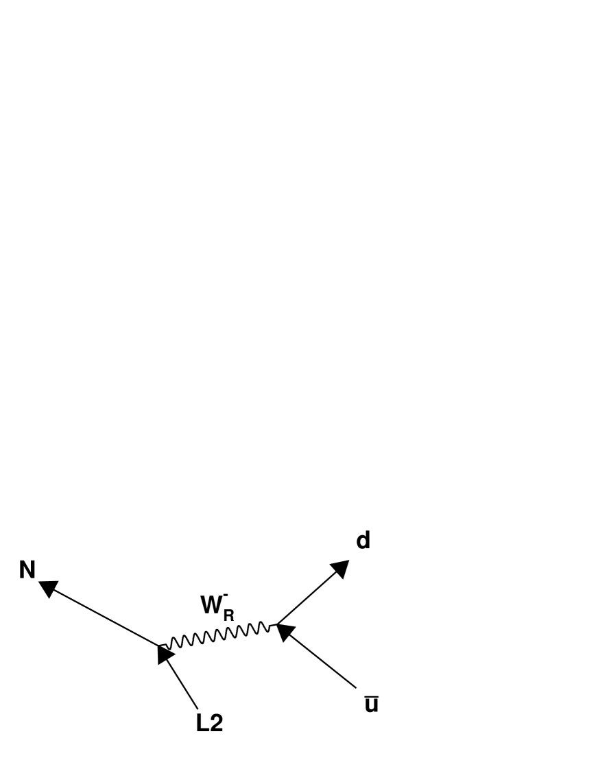
Figure 3: The process represented as two consecutive decays

In this section we calculate the width of this decay (it does not depend on the type of the neutrino). The expression for the amplitude is the following:

$$iM=\bar{v}_{N}\frac{ig}{\sqrt{2}}\gamma^{\mu}\frac{(1+\gamma^{5})}{2}v_{L}\frac{-i}{(q_{1}+q_{2})^{2}-M_{W}^{2}}$$

$$\left(g_{\mu\nu}-\frac{(q_{1}+q_{2})_{\mu}(q_{1}+q_{2})_{\nu}}{M_{W}^{2}}\right)\bar{u}_{d}\frac{ig}{\sqrt{2}}\gamma^{\nu}\frac{(1+\gamma^{5})}{2}v_{u}$$ (10)

Its squared modul can be simplified to

$$|M|^{2}=\frac{2g^{4}(Lq_{1})(k_{2}q_{2})}{\left(((q_{1}+q_{2})^{2}-M_{W}^{2})^{2}+M_{W}^{2}\Gamma_{W}^{2}\right)},$$ (11)

where $L$ is the momentum of the neutrino and the other momenta are the same as in the previous section. We substitute this formula into the general expression for the width of decay [6]

$$dw=\frac{1}{(2\pi)^{5}}\delta^{(4)}(k_{2}+q_{1}+q_{2}-L)|M|^{2}\frac{d^{3}\vec{k}_{2}d^{3}\vec{q}_{1}d^{3}\vec{q}_{2}}{16L^{0}k_{2}^{0}q_{1}^{0}q_{2}^{0}}$$ (12)

Again the delta-function of spatial momenta is taken off by integration over $q_{2}$. The delta-function of energy is also taken off in the same way. We rewrite

$$d^{3}\vec{q}_{1}=|\vec{q}_{1}|^{2}d|\vec{q}_{1}|\sin\theta d\theta d\varphi,$$

where $\theta$ and $\varphi$ is polar and axial angle of $\vec{q}_{1}$ relative to the vector $\vec{L}-\vec{k}_{2}$, and

$$L^{0}-k_{2}^{0}-q_{1}^{0}-q_{2}^{0}=\sqrt{\vec{L}^{2}+M_{\nu}^{2}}-|\vec{k}_{2}|-|\vec{q}_{1}|-\sqrt{|\vec{L}-\vec{k}_{2}|^{2}+|\vec{q}_{1}|^{2}-2|\vec{q}_{2}||\vec{L}-\vec{k}_{2}|\cos\theta}.$$

After integration over $|\vec{q}_{1}|$ we obtain that

$$dw=\frac{|M|^{2}|\vec{q}_{1}|\sin\theta d^{3}\vec{k}_{2}d\theta d\varphi}{(2\pi)^{5}16(|q_{1}|+|q_{2}|+|q_{1}+q_{2}|\cos\theta)|k_{2}+q_{1}+q_{2}||k_{2}|}$$ (13)

4 Description of the programs

We compare the angular distributions of the final state particles obtained using the full and simplified calculations. Two different programs perform the Monte-Carlo simulation of the process using the von Neumann’s method. The first program uses the cross-section formula obtained in section 2, the second one uses the simplified approach considered in section 3. More details of this simulation follow.

In this estimation we assume that the masses of $W_{R}$ and heavy neutrino are equal to 1000 GeV and 500 GeV correspondingly. These are typical values for the searches of these new particles at the LHC. For the moment we assume that the initial quarks have the same energy and opposite momentum directions so that the $W_{R}$ is produced at rest:

$$p1=\{E,0,0,E\},$$

$$p2=\{E,0,0,-E\},$$ (14)

where $E$ is the initial energy of quarks.

The first program has two similar versions: the first one considers the case of Dirac-like neutrino where only the reaction 1 can take place, the considers considers the case of Majorana-like neutrino where both reactions 1 and 2 happen with a probability of 50% each.

The maximum of the cross section is determined (maximization step) by the Monte Carlo method before the simulation step. At each iteration of the corresponding loops the final state particles 4-momenta take random values so that the energy and momentum are conserved. At the simulation step 2 or 4 loops are performed because antiquark can have positive or negative $p_{z}$ and because reactions 1 and 2 are possible in the Majorana neutrino case.

5 Results

In Figure 4 one can see the results. They are represented as a comparison of the distributions of the minimal distance $R$ in the $\eta-\phi$ plane from one of the final state leptons to one of the final state quarks. This distribution is important because in real collider experiments the efficiency of reconstruction drops when this distance is small (to exact zero when it is smaller than 0.5). The shape is different. To estimate the systematic error arising from the simulation as a decay chain we calculated the ratio of the number of events with $R>1$, where the drop of the lepton reconstruction efficiency due to the presence of a nearby jet is small, to the total number of events for the two simulations. They differ by 2.7%. This is our estimate of the systematic error of the simplified simulation. The difference between the cases of Dirac and Majorana heavy neutrinos is small (within 1%).

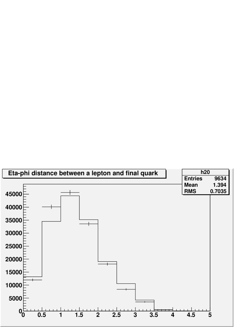
Figure 4: Distributions of the minimal distance in the $\eta-\phi$ plane from one of the final state leptons to one of the final state quarks. Histogram - from the simulation as a decay chain (statistical errors are negligible), points with errors - from the full matrix element with a Majorana heavy neutrino.

References

• [1] R.Mohapatra ’Unification and supersymmentry: the frontiers of Quark-Lepton physics’ Springer-Verlag, 1992
• [2] CMS-PAS-EXO-11-002 Search for a heavy neutrino and right-handed W of the left-right symmetric model in pp collisions at sqrt(s) =7 TeV
• [3] T.Β Sjostrand, S.Β Mrenna and P.Β Z.Β Skands, JHEP 0605 (2006) 026 [arXiv:hep-ph/0603175].
• [4] M.E.Peskin, D.V.Schroeder ’An introduction to Quantum field theory’, Westview Press, 1995
• [5] T.P.Cheng, L.F.Li Gauge Theory of elementary particle physics, Oxford University Press, New york, 1984
• [6] L.D.Landau, E.M.Lifshitz, Quantum electrodynamics, Pergamon Press, 1960
• [7] S. Weinberg. The Quantum theory of fields. Vol. 1: Foundations. Cambridge University Press, 1995.